Reproducible probe-level analysis of the Affymetrix Exon 1.0 ST array with R/Bioconductor

Abstract

The presence of different transcripts of a gene across samples can be analysed by whole-transcriptome microarrays. Reproducing results from published microarray data represents a challenge owing to the vast amounts of data and the large variety of preprocessing and filtering steps used before the actual analysis is carried out. To guarantee a firm basis for methodological development where results with new methods are compared with previous results, it is crucial to ensure that all analyses are completely reproducible for other researchers. We here give a detailed workflow on how to perform reproducible analysis of the GeneChip®Human Exon 1.0 ST Array at probe and probeset level solely in R/Bioconductor, choosing packages based on their simplicity of use. To exemplify the use of the proposed workflow, we analyse differential splicing and differential gene expression in a publicly available dataset using various statistical methods. We believe this study will provide other researchers with an easy way of accessing gene expression data at different annotation levels and with the sufficient details needed for developing their own tools for reproducible analysis of the GeneChip®Human Exon 1.0 ST Array.

INTRODUCTION

In the field of microarrays, it has traditionally been difficult to compare new methods with already established and published methods, as different strategies for preprocessing, summarizing and filtering make it almost impossible to work with the exact same data, even when the raw data is made available. That is why we consider reproducible research of fundamental importance as it will facilitate easy (i) revision of articles, (ii) access to data and results, (iii) communication with other researchers and (iv) comparison between different methods. Reproducible research is gaining relevance among the scientific community as shown by the number of articles published on the subject during the past years [1–4]. Ioannidis et al. showed that the results of only 2 of 18 published microarray gene-expression analyses were completely reproducible [5]. This is why some authors demand that documentation and annotation, database accessions and URL links and even scripts with instructions are made publicly available [2]. Journals like Biostatistics have even appointed an Associate Editor for reproducible research, but still treat it as a ‘desirable goal’ rather than a requirement [6]. Setting up a framework for reproducible research necessarily implies working with free and open-source software, for example, R/Bioconductor [7, 8]. Additionally, using Sweave [9, 10] (a tool for embedding R code in LATEXdocuments [11]) enables automatic reports that can be updated with output from the analysis.

The main tool in this article will be the Bioconductor package aroma.affymetrix [12] that can analyse all Affymetrix microarray types with a Chip Definition File (CDF file). Affymetrix sometimes refer to their microarrays as ‘chips’. The number of arrays (samples) that can be simultaneously analysed by aroma.affymetrix is virtually unlimited, as the system requirements are just 1 GB RAM, for any operating system [13]. This package is freely available and can easily be installed into R. The aroma.affymetrix website www.aroma-project.org is conceived as reference for all the possible microarrays that can be analysed with aroma.affymetrix, and does not focus specifically on the analysis of the GeneChip® Human Exon 1.0 ST Array (or exon array in short). Portable scripts for a fast and basic analysis can be obtained on request to aroma.affymetrix’s authors.

The analysis of exon array data in R/Bioconductor is not yet standard. There are several packages available, and it can be a tremendous effort for a newcomer to maneuver between them and to overcome the numerous challenges associated with these packages. This article aims to make this task easier and to provide a quick reference guide to aroma.affymetrix’s documentation. We also explain how to extract data for different statistical analyses and propose a method for gene annotation and for gene profile visualization. For this last step, we use the packages biomaRt and GenomeGraphs to annotate and visualize the transcripts in a genomic context. When using the workflow, please remember to cite packages aroma.affymetrix, GenomeGraphs and biomaRt.

In this article, we sketch the proposed workflow, which is carried out solely in R/Bioconductor, and explain some key sections. The complete code is available as a Sweave (.Snw) [9] document that will allow the reader to reproduce our exact results. The .Snw document can also be converted into an R script and executed. The workflow starts by reading in the data, followed by background correction and quantile normalization. We then explain how to obtain transcript cluster-, probeset- and probe-level estimates. Afterwards, different methods for the statistical analysis of differential splicing or differential gene expression are reviewed. Finally, we make a suggestion on how to annotate transcript clusters to genes in the lists obtained from the statistical analyses, and how to plot the data including genomic information. To exemplify the use of the workflow, an example dataset [14] is analysed along the way.

BACKGROUND ON ALTERNATIVE SPLICING

Splicing is the post-transcriptional process that generates mature eukaryotic messenger RNAs (mRNAs) from pre-mRNAs by removing the non-coding intronic regions and joining together the exonic coding regions. For many genes, two or more splicing events take place during maturation of mRNA molecules, resulting in a corresponding number of alternatively spliced mRNAs. These mature mRNAs translate into protein isoforms differing in their amino acid sequence and ultimately in their biochemical and biological properties [15, 16]. Alternative splicing is one of the main tools for generating RNA diversity, contributing to the diverse repertoire of transcripts and proteins [16, 17]. It is known that 92–94% of multi-exon human genes are alternatively spliced and that 85% of those have a minor isoform frequency of at least 15% [18, 19]. In our case, we will focus on the detection of differential splicing between groups, as for instance tissue types, or healthy versus diseased samples.

The exon array was presented in October 2005 as a tool for the analysis and profiling of whole-transcriptome expression [20–22]. To interrogate each potential exon with at least one probeset, the exon array contains about 5.6 million probes grouped into >1.4 million probesets (most probesets consisting of four probes), which are further grouped into 1.1 million exon clusters, or collections of overlapping exons. Finally, exon clusters are grouped into >300 000 transcript clusters to describe their relationship, for example, shared splice sites or overlapping exonic sequences. Each gene is covered, on average, by 40 probes interrogating regions located along the entire gene [23]. This probe positioning aims at providing better estimates of gene expression levels than previous arrays, and allows for the study of differential splicing [24] and differential gene expression based on summarized exon expression.

The exon array has three levels of annotation for the interrogated transcript clusters: core, extended and full [25]. Core transcript clusters are supported by the most reliable evidence such as RefSeq transcripts and full-length mRNAs [26], and a core transcript cluster is roughly a gene [27]; the extended level contains the core transcript clusters plus complementary DNA (cDNA)-based annotations [28], and the full level contains the two previous levels plus ab initio, or algorithmic, gene predictions [29]. It is worth noting that aroma.affymetrix enables the analysis at the three levels of annotation mentioned above, and also that it provides intensity estimates for probes, probesets and transcript clusters, allowing for a variety of options for the analysis.

WORKFLOW

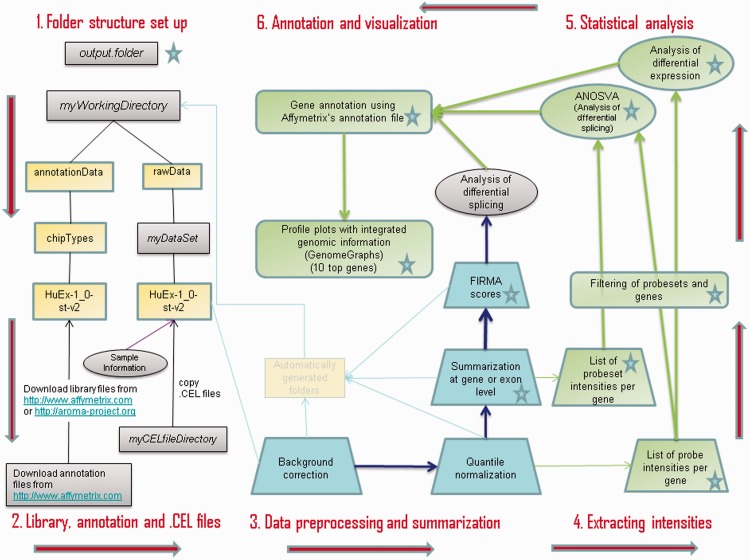
Our workflow for the analysis of exon array data starts by setting up the required folder structure for aroma.affymetrix. The data are then preprocessed and summarized at transcript cluster and/or probeset level. Next, transcript clusters are analysed with several statistical models to detect differential expression or splicing, and the transcripts of interest are annotated and visualized at the end (Figure 1). In the code, places where user input is needed are marked by ‘***’, and places where the user can choose whether to modify parameters are marked by ‘**’.

Figure 1:

Flowchart for an analysis with aroma.affymetrix, read counterclockwise starting in upper left corner: 1. and 2.; folder structure set-up including library, annotation and .CEL files; 3. data preprocessing and summarization; 4. extraction of intensities at transcript cluster, probeset and probe level, including filtering recommended by Affymetrix; 5. statistical analysis of differentially expressed or spliced transcript clusters and 6. annotation and visualization of transcript cluster profiles. Blue boxes (step 3.) represent parts of the analysis implemented in aroma.affymetrix, yellow and green boxes are part of the code provided in this article and purple boxes represent user-input needed (steps 1., 2. and analysis of differential splicing with FIRMA). Output produced at several steps is saved in user-chosen ‘output.folder’ and represented by a star shape in the workflow. A number of folders are automatically generated by aroma.affymetrix (represented by a faded yellow rectangle in 3.); our workflow does not make use of the contents of such folders.

To exemplify the use of the tutorial, we have used Affymetrix’s colon cancer dataset [14], consisting of a collection of paired samples of colon tumour tissue and adjacent normal tissue from 10 patients and available at http://www.affymetrix.com/support/technical/sample_data/exon_array_data.affx. According to Affymetrix’s website, the RNA samples are from a commercial source. This dataset has been used in a number of articles to evaluate the performance of different analysis methods [30–33], and a number of genes have been validated to be differentially spliced or not [14]. The analysis was performed in R version 2.15.1 (32 bit).

Start by installing and loading aroma.affymetrix in R and loading the other libraries required:

• > source(“http://aroma-project.org/hbLite.R”)

• > hbInstall(“aroma.affymetrix”)

• > require(aroma.affymetrix)

• > require(biomaRt)

• > require(GenomeGraphs)

Setting up the structure and files for the analysis workflow

This section corresponds to steps 1 and 2 in Figure 1. The first step is to create the folder structure: under a main folder of our choice—‘myworkingDirectory’—we will create the ‘rawData’ and ‘annotationData’ folders, which will be common to all aroma.affymetrix projects. Inside ‘annotationData’, the subfolder ‘chipTypes’ will contain one subfolder per chip type, with the exact name of the .CDF file provided by Affymetrix, ‘HuEx-1_0-st-v2’ in our case. Inside this folder, we will save any library and annotation files that might be needed. Besides, the ‘myDataSet’ folder will be created under ‘rawData’ to store .CEL files. These files are the output of a microarray experiment and contain the result of the intensity calculations per probe or pixel. Note that the microarray experiment produces one .CEL file per array and that one array analyses one sample. Note also that we need one ‘myDataSet’ folder per experiment and that ‘myDataSet’ will be added as a tag at the end of the aroma.affymetrix output.

• > #*** user-defined working directory

• > wd <- “myWorkingDirectory”

• > #*** user-defined data set name

• > ds <- “myDataSet”

In the second step, we save our library (.CDF in our case) and .CEL files in the corresponding folders. Affymetrix’s unsupported CDF files can be downloaded from http://www.affymetrix.com/Auth/support/downloads/library_files/HuEx-1_0-st-v2.cdf.zip; note that registration is needed. For the exon array, Elizabeth Purdom has created a number of binary .CDF files based on Affymetrix’s text CDF file [13] that are faster to query and more memory efficient. Such binary .CDF files for core, extended and full sets of probesets can be downloaded from http://aroma-project.org/node/122. In the example below, we use the custom aroma file for core transcript clusters, which might be updated in the future. Our original .CEL files will be copied from the user-specified ‘myCELfileDirectory’ into the exon ‘rawData’ subfolder (the code is part of the .Snw version of this article). The desired output folder specified in ‘output.folder’ should exist in advance.

• > #** download user-defined library file

• > library.file <-

• +  paste(annotation.data.exon,

• +    “HuEx-1_0-st-v2,coreR3,

• +    A20071112,EP.cdf”,sep = “/”)

• > download.address <-

• +   “http://bcgc.lbl.gov/cdfFiles/”

• > file <- paste(“HuEx-1_0-st-v2,A20071112,EP”,

• +     “HuEx-1_0-st-v2,coreR3,

• +     A20071112,EP.cdf”,sep = “/”)

• > custom.cdf <-

• +   paste(download.address, file, sep = ””)

• > download.file(url = custom.cdf,

• +      destfile = library.file,

• +      mode = “wb”, quiet = FALSE)

• > #*** user-defined directory containing .CEL

• +       files

• > cel.directory <- “myCELfileDirectory”

• > #*** user-defined output folder

• > output.folder <- “output.folder”

In addition, the sample information should be saved in a tab-separated file with column names celFile, replicate and treatment containing .CEL file name (without .CEL), replicate identifier and treatment name, respectively. This file should be called ‘SampleInformation.txt’, and it will be copied from the user-specified directory into the ‘\rawData\myDataSet \HuEx-1_0-st-v2’ folder (which will also contain the .CEL files) after it has been created. The sample information file for the colon cancer example is attached as an additional file.

• > sample.info <-

• +   read.table(file = paste(raw.data.exon,

• +    “SampleInformation.txt”, sep = “/”),

• +      sep = “\t”, header = TRUE)

Finally, NetAffx transcript clusters’ and probesets’ annotation files should be saved in ‘annotationData/chipTypes/HuEx-1_0-st-v2’. We have used release 32, which was most up to date at the time of writing, and we downloaded files ‘HuEx-1_0-st-v2.na32.hg19.transcript.csv.zip’ and ‘HuEx-1_0-st-v2.na32.hg19.probeset.csv.zip’ from http://www.affymetrix.com/estore/browse/products.jsp?productId=131452&categoryId=35676&productName=GeneChip-Human-Exon-ST-Array#1_3, Technical Documentation tab, under NetAffx Annotation Files. The extracted .csv files should be converted into .Rdata files for querying them faster in the future. Note that the number of lines to skip might differ for future annotation files.

• > transcript.clusters.NetAffx.32 <-

• +   read.csv(file = paste(annotation.data.

• +    exon,HuEx-1_0-st-v2.na32.hg19.

• +    transcript.csv”,sep = “/”), skip=24)

• > probesets.NetAffx.32 <-

• + read.csv(file = paste(annotation.data.exon,

• +    “HuEx-1_0-st-v2.na32.hg19.

• +     probeset.csv”,sep = “/”), skip=23)

Data preprocessing and summarization to probeset/transcript cluster level

After defining chip type and dataset, background correction and quantile normalization are carried out as shown in Figure 1, step 3. In these preprocessing steps, it is possible to use either Affymetrix’s original .CDF file, the .CDF files provided by the aroma project (the file for core transcript clusters in our example) or a .CDF file created by the user. The summarization step, however, must be done using one of the custom .CDF files available at the aroma.affymetrix project website.

Background correction as defined by Irizarry [34] and quantile normalization are performed by the RmaBackgroundCorrection() and QuantileNormalization() functions, respectively. The raw, background corrected and quantile normalized probe intensities can be visualized using the plotDensity() function applied to the corresponding object. Summarization is done with the ExonRmaPlm function [35]. The parameter mergeGroups determines whether to summarize at transcript level (TRUE) or probeset level (FALSE). All the functions described automatically create subfolders such as ‘plmData’ or ‘probeData’ inside ‘myWorkingDirectory’. A more detailed version of this code with interesting comments about the choice of .CDF and possibilities for quality control is available at http://www.aroma-project.org/vignettes/FIRMA-HumanExonArrayAnalysis.

• > chipType <- “HuEx-1_0-st-v2”

• > #** user-defined .CDF file: change tags

• +    parameter

• > cdf <- AffymetrixCdfFile $ byChipType, tags=

• + (chipType,“coreR3,A20071112,EP”)

• > cs <- AffymetrixCelSet$byName(ds, cdf = cdf)

• >

• > # background correction

• > bc <- RmaBackgroundCorrection(cs)

• > csBC <- process(bc, verbose = verbose)

• >

• > # quantile normalization

• >  qn <- QuantileNormalization(csBC,

• +          typesToUpdate = “pm”)

• > csN <- process(qn, verbose = verbose)

• >

• > # summarization

• > # transcript cluster level

• > plmTr <- ExonRmaPlm(csN, mergeGroups = TRUE,

• +         tag = “coreProbesets

• +         GeneExpression”)

• > # probeset/exon level

• > plmEx <- ExonRmaPlm(csN, mergeGroups = FALSE,

• +         tag=“coreProbesetsExon

• +         Expression”)

Extraction of intensity estimates

The aroma.affymetrix documentation focuses on analyses at the probeset and transcript cluster levels. The respective intensities are obtained by applying the function getChipEffectSet() to the transcript or probeset plm objects (plmTr and plmEx, respectively) and then extracting the corresponding dataframes. However, it is also possible to extract the background-corrected and quantile-normalized intensities of all probes using the function getUnitIntensities. While plmTr is suitable for the FIRMA analysis, plmEx is well suited for probeset-level analysis. For the ANOSVA probe analysis described in the statistics section, we have created one list of dataframes containing probe intensities per transcript cluster, and another list of dataframes containing probeset intensities per cluster (code included in .Snw).

• > # extract a matrix of gene intensities

• > cesTr <- getChipEffectSet(plmTr)

• > trFit <- extractDataFrame(cesTr,

• + addNames=TRUE)

• > # extract a matrix of probeset intensities

• > cesEx <- getChipEffectSet(plmEx)

• > exFit <- extractDataFrame(cesEx,

• + addNames=TRUE)

• > # extract a list of probe intensities per gene

• > unitIntensities <-

•          readUnits(csN, verbose=verbose)

The high number of transcript clusters analysed in combination with the usually small number of chips tends to cause a high number of false positives [25]. To reduce the number of false positives, Affymetrix recommends to perform detection above background (DABG) [36] on the dataset before the analysis [25]. The DABG procedure is not implemented in aroma.affymetrix, so we decided to follow the procedure described in [30] and use 3 as a threshold for the probeset intensity, so that probesets with a intensity below 3 will be marked as absent. Except for this change, we followed the guidelines proposed in [25] to remove absent transcript clusters and probesets, where neither probesets that are absent in more than half of the samples of a group nor transcript clusters with more than half of the probesets absent are analysed.

Besides this filtering based on expression levels, another filtering step that removes probesets presenting cross-hybridization is advisable [25]. Cross-hybridizing probesets are identified in file ‘HuEx-1_0-st-v2.na32.hg19.probeset.csv’ and removed. Affymetrix recommends to filter them out after the analysis, but we have decided not to include them in the analysis to narrow down the number of probesets/transcript clusters to investigate.

The filtering procedure is part of the .Snw file. In our example, where we analysed only core probesets, 136 233 probesets of 284 258 were deemed present by our filter, and the number of transcript clusters to analyse (present in both samples) was reduced from 18 708 to 8401.

Statistical analysis

In this section, we give an overview of model-based statistical methods available for the analysis of differential splicing and suggest a method for the analysis of differential gene expression, and the analyses are done genewise.

Differential splicing

The models used in this article are extensions of the linear model by Li and Wong [37]

(1)

where y_pt is the intensity measure of probe p for treatment t, is a probe affinity term, is the gene-level estimate for treatment t and is the error term.

ANOSVA (Analysis of Splicing Variation) was presented by Cline et al. [38] and is a two-way ANOVA model with probeset and treatment as factors:

(2)

where y_pet is the intensity measure of probe p in probeset e and treatment t, the overall mean μ is the baseline level of all probes in all experiments and and are the probeset and treatment effects. The interaction term indicates whether the effect of the probeset depends on the treatment and is therefore key to the detection of differential splicing.

The model in (2) can be extended to include random effects associated to replications from the same individual, r:

(3)

where I_r is the random effect of each individual r and C_tr is the random chip effect. The error terms are independent, identically distributed (i.i.d.) -distributed.

Under the null hypothesis of no differential splicing, the s will all be zero, and therefore we consider the test statistic

where is the estimate for , and is the standard error of . Large values will be critical for the null hypothesis. Under the model assumptions, t will follow a distribution [39, Chap. 5], with N the total number of observations per transcript cluster, T the number of treatments, n_e the number of probesets in the transcript cluster and R the number of individuals. For each gene, the smallest P-value from the above t-tests is regarded as a measure of confidence that the gene is differentially spliced across the experimental conditions [38]. The interaction estimates and variances and thus the test statistics are contrast dependent, so choosing a different contrast will alter the gene lists. In our analysis, we have used the sum contrast available in R, where parameter estimates are centred around zero.

We use lm to fit the model in equation (3) to the probe-level estimates obtained using unitIntensities() from aroma.affymetrix to 8075 multi-exonic transcript clusters. Here, we only show the code corresponding to equation (3), the rest of the code is part of the .Snw file.

• > # ** user-defined parameters for linear model

• > lm <-

• +   lm(intensity ∼ probeset + treatment +

• +   C(probeset:treatment, contr.sum)

• +   replicate/treatment

• > n.probesets <-

• + length(unique(dataframe$probeset))

• > main.effects <-

• +        1 + (n.probesets - 1) +

• +       (length(unique(dataframe

• +       $treatment)) - 1)

• > DS.parameters <- (n.probesets - 1)*

• +       (length(unique(dataframe

• +       $treatment)) - 1)

• > p.t <-

• +   min(summary(lm) $

• +   coefficients[(main.effects+1):

• +   (main.effects + DS.parameters),

• +   “Pr(>|t|)”])

Although the vast majority of probesets contain four probes, transcript clusters containing probesets with less than four probes will give rise to an unbalanced design. Nevertheless, the t-distribution is almost a normal distribution for long transcript clusters so the unbalanced design does not have any practical implications. For shorter transcript clusters, however, an unbalanced design might be a problem.

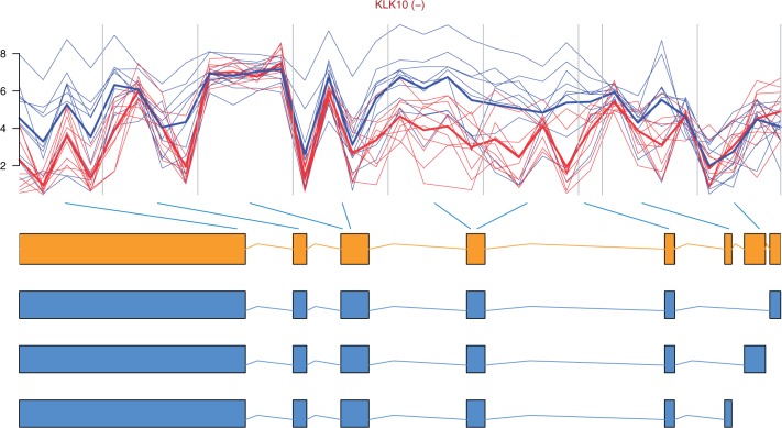
The top 10 most differentially spliced genes, sorted by the minimum P-value of their t-tests, appear in Table 1. The gene ZAK was validated as differentially spliced in [14]. See Figure 2 for the profile plot of KLK10, where the thick lines representing the mean intensity in each group have been plotted for easing the interpretation. Note that there is one measurement per probe in each probeset, typically four probes per probeset. How to obtain such plots is described in the annotation and visualization section below. The genes in Figures 2, 3, 4 and 6 were chosen because they span over a shorter genomic region and show a clearer picture of the relationship between probesets and exons than the other genes in the lists of top 10 genes.

Table 1:

Top 10 differentially spliced genes with minimum P-values from the ANOSVA probe model, equation (3)

Genes highlighted in grey appear in Figures 2 and 5.

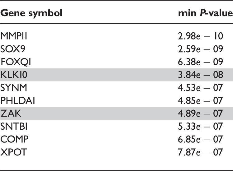Figure 2:

Profile plot of gene KLK10 with the gene model and possible transcripts retrieved from Ensembl [50]. The (−) next to the gene name indicates that it is located on the reverse strand. The mean intensities of each group are plotted with a thicker line. Exons 5 (mapped by probesets 4 and 5) and 8 (mapped by probeset 9), counted from the 5′ end, seem to be higher expressed in tumour samples (blue/dashed) than in normal (red/solid).

Figure 3:

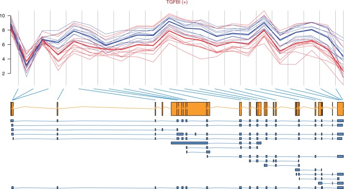
Profile plot of TGFBI with the gene model and transcripts retrieved from Ensembl [50]. The gene is on the forward strand as indicated by (+) next to its name. The mean intensities of each group are plotted with a thicker line; note that only one estimate is plotted by probeset, and it corresponds to the estimate computed by ExonRmaPlm(…, mergeGroups=FALSE). Here, it seems like the tumour samples (blue/dashed) present increased expression from exon 3 until the end of the transcript, with respect to normal (red/solid) samples. Given that TGFBI is on the forward strand and that the difference is at the beginning of the transcript, we might be observing a case of alternative promoter usage.

Figure 4:

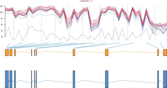
Profile plot of gene LGALS4 with the gene model and transcripts retrieved from Ensembl [50], the gene is on the reverse strand. Interestingly, this gene only has one transcript. We might then be facing a novel splicing event or, more likely, a false positive detected by the method.

Figure 6:

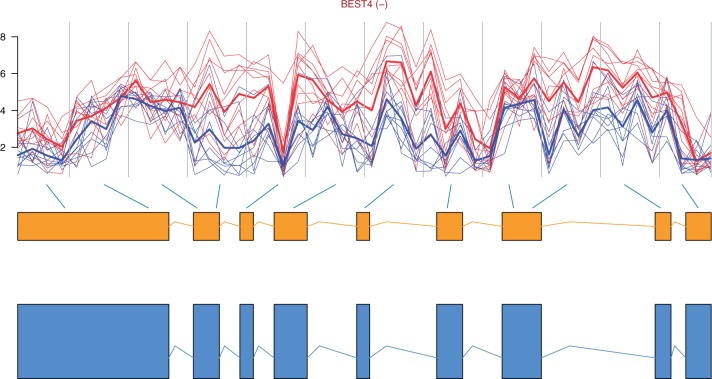
Profile plot of gene BEST4, which is on the reverse strand, with the gene model and transcripts retrieved from Ensembl [50]. The gene is under expressed in tumour (blue/dashed) compared with normal (red/solid) samples.

A slight variation of ANOSVA is the probeset model as implemented in Partek [40] (note that the probe subscript p has been removed):

(4)

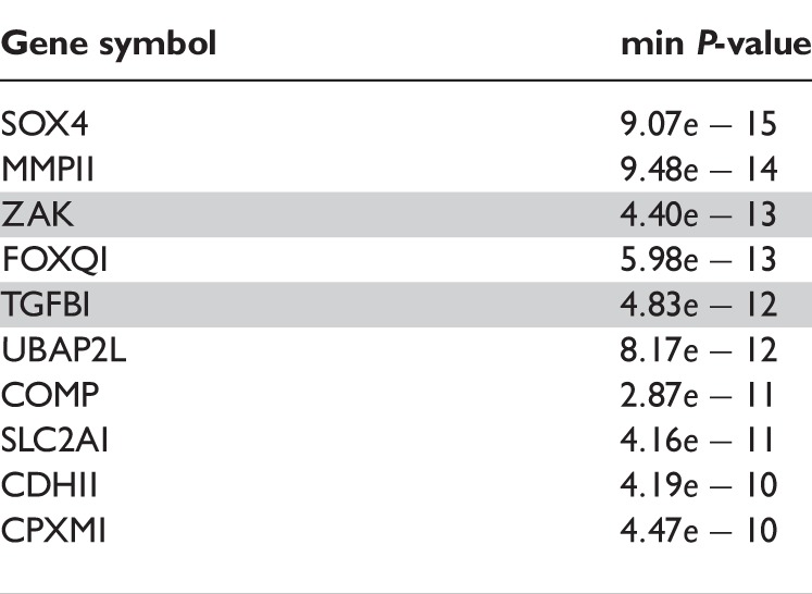
For the probeset-level ANOSVA, we used the probeset-level estimates obtained by affyPLM(…, mergeGroups = FALSE). After filtering for non-present or cross-hybridizing probesets, and absent transcript clusters, we were left with 8189 transcript clusters to study. These clusters are sorted according to the minimum P-value of the individual t-test scores for differential splicing, and the top 10 genes obtained appear in Table 2. The genes MMP11, ZAK and COMP are in the top 10 genes for both the ANOSVA probe and the ANOSVA probeset models. Gene TGFBI appears in Figure 3.

Table 2:

Top 10 differentially spliced genes with minimum P-values from the ANOSVA probeset model, equation (4)

Genes highlighted in grey appear in Figures 3 and 5.

FIRMA (Finding Isoforms using Robust Multichip Analysis) was first introduced by Purdom et al. [30] for the exon array. In presence of differential splicing, the model in (1) will not fit and this will show up in the residuals. The linear model used is the following:

(5)

with the probe affinity, the gene-level effect for chip tr and the error terms are i.i.d. -distributed. Note that in contrast to the model in (3), we do not compute an overall gene-level estimate, but a gene-level estimate per chip.

In model (5), like in model (1), there is no treatment/probeset interaction term, so differential splicing is analysed probesetwise using the residuals per probeset e:

(6)

where and are the estimates of and .

The median of the standardized residuals per probeset per chip is chosen as score statistic:

(7)

The standardization with the median absolute deviation of the residuals per gene makes the scores comparable across genes.

The FIRMA scores are extracted from the plmTr object obtained in the data pre-processing and summarization step. All probesets and transcript clusters were analysed by FIRMA, as it is part of the default aroma.affymetrix workflow.

• > firma <- FirmaModel(plmTr)

• > fit(firma, verbose = verbose)

• > fs <- getFirmaScores(firma)

• > firma.scores <- extractDataFrame(fs)

After obtaining the FIRMA scores per probeset per sample, we proceeded as described in [30]: (i) For each probeset, we took the difference of FIRMA scores for each of the 10 pairs of normal/cancer samples and (ii) calculated the mean of the 10 differences per probeset. Then (iii) we ranked the probesets according to their absolute mean difference: as the scores are comparable across transcript clusters, larger average differences between the normal and cancer samples will point at exons more differentially spliced between the two conditions. The resulting list was filtered to keep only probesets and transcript clusters that had passed the filter described in the filtering section above; the code is part of the .Snw file. To get a gene list instead of a probeset list as in [30], we mapped probesets to transcript clusters and then selected the top 10 genes on the list (Table 3). The profile plot of gene LGALS4 appears in Figure 4. The high average difference for this gene is owing to a FIRMA score of 830 030.8 at probeset 3 861 578 corresponding to the tumour sample of replicate 7.

Table 3:

Top 10 differentially spliced genes and their top scores from the FIRMA model, equations (5) to (7)

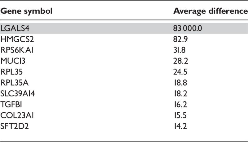Gene LGALS4, highlighted in grey, appears in Figure 4.

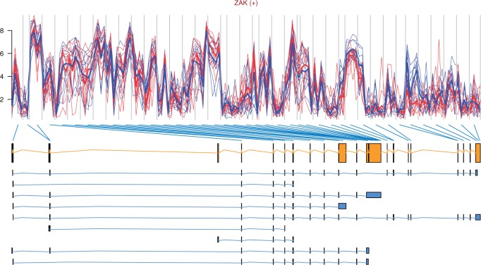
Of 14 genes investigated for differential splicing in ([14], Table 1), 10 passed our filtering procedure and were analysed for differential splicing: ACTN1, VCL, CALD1, SLC3A2, COL6A3, CTTN, FN1, MAST2, ZAK and FXYD6. The gene ZAK appears in the top 10 genes from ANOSVA probe and ANOSVA probeset, but a plot is not produced automatically by the code because ZAK is not recognized by BioMart. Instead, we looked the gene up in PubMed obtaining the Ensembl ID: ENSG00000091436 and used this to plot the gene (Figure 5). The gene COL6A3 appears among the top 100 genes for the ANOSVA probe and the ANOSVA probeset methods. Gene ACTN1 is among the top 100 genes for ANOSVA probeset and it is also the first of Gardina’s genes to appear in the filtered FIRMA list, at position 154.

Figure 5:

Profile plot of gene ZAK with the gene model and transcripts retrieved from Ensembl [50]. The gene is on the forward strand. There seems to be a differential splicing event identified by probesets 35 and 36 (counted from the 5′ end of the gene), corresponding to exons 19 and 20.

The differences in the gene lists obtained with ANOSVA and FIRMA are caused by the distinct nature of the two methods. ANOSVA was designed to look for splicing changes that are consistent within replicate sets, and differential splicing is assessed by the significance of a statistical test. FIRMA is a robust method that can detect splicing chances not necessarily consistent within replicate sets and so does not explain how to summarize from exon-sample scores to overall gene-level scores or whether it is recommended to do so. This implies some arbitrariness in the summarization procedure, which makes FIRMA less reproducible than ANOSVA. A thorough benchmarking of ANOSVA, FIRMA and several other methods for detecting differential splicing can be found in [41]. The comparison is done by means of receiver operating characteristic curves on two datasets: a panel of 11 human tissues with confirmed alternative splicing events; and a modification of a spike-in experiment where 25 transcripts were hybridized to HeLa cells [42, 43]. In most of the experiments carried out, FIRMA seems to perform better than ANOSVA. In [44] and in [45], ANOSVA and FIRMA are compared with other methods, respectively, but not with each other.

Differential gene expression

In this section, we analyse differential gene expression using probe-level data. We study two types of transcript clusters: (i) the ones not included in the ANOSVA probe analysis above (with only one probeset or not present in both normal and cancer groups) and (ii) the ones not showing differential splicing (ANOSVA probe P-value above 0.1). The analysis of group (ii) is based on the hierarchical principle: only look for significant main effects (differential expression in this case) among those transcript clusters with no significant interaction terms (differential splicing) [46 (p. 427)]. In total, we analysed 16 231 transcript clusters. We fit the following linear model to those transcript clusters:

(8)

where is the gene-level treatment effect, is a parameter that captures probesets expressed above or below the overall transcript cluster level and I_r and C_tr are random effects for patient and chip, respectively.

• > aov <-

• +   aov(intensity ∼ probeset + treatment +

• +        Error(replicate+

• +        replicate:treatment))

• > p.F <-

• +  summary(aov)$ “Error: Within”[[1]]

• + [“treatment”,“ Pr(>F) ”]

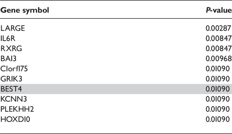
The null hypothesis is that the gene expression is the same in all groups. The top 10 genes, with adjusted P-values, appear in Table 4. The method used for adjusting the P-values was Benjamini-Hochberg’s correction [47] using the function p.adjust(..., method = “BH”). Only 80 of 159 genes appearing in Gardina’s list of genes up- and down-regulated in tumour ([14] additional file 1) passed our filters and were analysed for differential gene expression. Among those analysed, the genes CLDN1, SST, MUSK, KIAA1199 and SLC30A10 were in the top 100. The gene BEST4 is shown in Figure 6. This gene is down-regulated in tumour (blue or dashed in the printed version) compared with normal (red or solid in the printed version) samples. The thicker lines represent the mean expression levels in the two groups.

Table 4:

Top 10 differentially expressed genes from (8) with corrected P-values. Gene BEST4, highlighted in grey, appears in Figure 6

Gene annotation and visualization

We chose to annotate transcript clusters to genes using the NetAffx transcript cluster annotation release 32 specified above using the AnnotateGenes() function. Some transcript clusters present unspecific annotation and have several possible associated gene names. We have decided to remove such clusters from our output, as we cannot map them uniquely to a gene and afterwards interpret the result according to the gene structure. The number of transcript clusters presenting non-unique annotation to genes was 1147 out of 8189 for the differential splicing analyses and 2917 out of 16 231 in the differential expression analysis.

After gene annotation, the user can select genes for visual inspection. Visual inspection of candidates for differential splicing is recommended by Affymetrix as a way to identify possible false positives [25]. Plots of gene profiles with integrated genomic information are obtained using the biomaRt [48] and GenomeGraphs [49] packages in Bioconductor.

We use bioMart to connect to the latest version of the Homo sapiens dataset in Ensembl [50] (Ensembl genes 68, GRCh37.p8 at the time of writing) and retrieve genes by their HGNC symbol [51]. Gene and exon structures are imported from Ensembl. Gene and Exon objects are created by makeGene() and makeTranscript() from GenomeGraphs. We store expression data and probeset start and stop positions in an ExonArray object by makeExonArray(). The final plot is created passing a list with the objects created to the gdPlot(list(exon, gene, transcript,…)) function.

Our plots show on top the gene HGNC symbol followed by (+) for genes on the forward strand and by (−) for those on the reverse strand. Below, the plot of probeset intensities appears with vertical lines delimiting probesets. Note that for models based on probe-level data (ANOSVA probe, FIRMA and differential expression), the intensities of all probes in the probeset (1–4) are shown. Samples from the same treatment group appear in the same colour, red/solid for normal samples and blue/dashed for tumour samples in this case. For the genes detected by the ANOSVA probe, the ANOSVA probeset and the differential expression methods, thin lines show the expression level of each sample, whereas the thicker lines show the mean intensities in each of the groups. Immediately after the profile plot, the gene model retrieved from Ensembl is shown in orange, followed by the possible transcript model(s) in blue. The gene model consists of the exons that appear in all possible transcript models. Exons (boxes) in the gene model are linked by blue lines to the probesets above, indicating which probeset(s) interrogate which exon (Figures 2–6).

DISCUSSION

The aim of this article was to give a tutorial on how to perform a complete and reproducible analysis of exon array data in R/Bioconductor. We have worked with three packages: aroma.affymetrix, biomaRt and GenomeGraphs to go from .CEL files to intensity data, statistical analysis, annotation and visualization. The packages were chosen for their flexibility and ease of integration. We believe that our workflow covers a number of analysis variants for the exon array, including differential splicing analysis at probe and probeset-level and differential expression analysis at probe level, and gives the user the opportunity to focus on all or only some of the aspects of the data analysis. We make our entire code available so that other researchers can use it as it is or adapt it to their needs.

Some possible modifications to the workflow include background correcting by subtracting from each probe the median intensity of all the exon array control probes with the same GC content, or removing noisy arrays identified in the quality control step. The latter can be easily done by removing such arrays from the sample information file and re-doing the background correction and normalization steps. A package in R for fitting linear and generalized linear mixed-effects models is lme4 [52]. In our case, we used lm instead of lmer because it is faster, but it requires a balanced design. Finally, differential gene expression could be analysed using the gene-level estimates obtained from the plmTr object in other R packages such as limma [53]. Another extension of the workflow could include a general analysis strategy of the FIRMA scores, which in this study was tailor-made for a two-treatment scenario.

Different Bioconductor packages could have been used in some of the analysis steps. For example, xmapcore [54] provides annotation data and cross-mappings between genetic features such as transcript clusters or exons and Affymetrix probesets. This package, however, requires the separate installation of a MySQL database, which makes this a more complex alternative than the one we have chosen. The xps package [55] could have been used for data preprocessing and summarization, but it requires the installation of the ROOT framework [56], and a certain level of understanding of ROOT files and ROOT trees is recommended. Our workflow does not require any prior knowledge beyond R/Bioconductor. Other free software includes BRB-Array Tools [57], based on R, C, Fortran and Java, with an Excel front end, and dChip [58], which is written in Visual C++ and developed for Windows, although some users have been able to run it on Mac and Unix computers.

A previous article on exon arrays [24] suggests a pragmatic approach and does the analysis piecewise, starting with Affymetrix Power Tools (APT) and then exporting the data to R. We recognize this is a fix for the lack of straightforward packages for dealing with the exon array in Bioconductor. However, it implies working with several pieces of software so we do not find it fit for reproducible research. Licensed software, like Partek [40] or GeneSpring GX [59], has been used in other studies [22, 60]. In contrast to licensed software, R/Bioconductor is free and available for anyone, it allows the user to control most analysis options and it enables customizable and reproducible analyses that are more easily reviewed. Still, the aroma.affymetrix package does not provide the speed of APT or the licensed software, and it requires more user input. Nevertheless, with this code and minimal user input, any dataset can be analysed regarding differential expression at probe level and differential splicing using the ANOSVA model.

Although the profile plots generated with GenomeGraphs are highly informative, they can be difficult to interpret for genes spanning over a long genomic region, for example, TGFBI in Figure 3 and ZAK in Figure 5. In our opinion, showing 3′ and 5′ ends, and exon and probeset numbers would significantly improve the readability of the plots. Actually, GenomeGraphs allows to add the Affymetrix probeset identity below the profile plots, but we believe that a probeset numbering relative to the gene over the profile plot would be preferable. In the future, it would also be interesting to study the flexibility of the output imported from Ensembl and, for example, remove the intronic regions from the gene and transcript models in the graphical representations.

SUPPLEMENTARY DATA

Supplementary data are available online at http://bib.oxfordjournals.org/.

Key points.

• The analysis of exon array data in R/Bioconductor is not yet well established.

• Reproducible research is fundamental to guarantee that methods can be compared on an equal footing, a framework for reproducible research is therefore needed.

• With minor modifications, the code provided with this article can be used to analyse any dataset.

• We give an overview of model-based methods for the analysis of differential splicing.

• A publicly available dataset is analysed to exemplify the use of the code, including gene annotation and representation, and the methods for differential splicing.

Biographies

Maria Rodrigo-Domingo is a PhD student in biostatistics at the Department of Mathematical Sciences of Aalborg University. Her project focuses on the improvement of the statistical methods for the detection of differential splicing using Affymetrix’s exon array.

Rasmus Waagepetersen is a professor in statistics at the Department of Mathematical Sciences of Aalborg University with research interests in spatial statistics, simulation based inference, generalized linear mixed models and quantitative genetics.

Julie Støve Bødker holds a PhD in molecular biology and she is a post-doc researcher at the research laboratory of the Department of Haematology, Aalborg University Hospital. Her work includes analysing microarray platforms from Affymetrix, with a focus on DLBCL.

Steffen Falgreen is a PhD student in biostatistics at the research laboratory of the Department of Haematology, Aalborg University Hospital. In his project, he is developing new statistical models for the prediction of chemotherapy outcome on DLBCL.

Malene Krag Kjeldsen holds a PhD in medicine and she is a post-doc researcher at the research laboratory of the Department of Haematology, Aalborg University Hospital. She works with transcription factors known to be involved in B-cell differentiation and DLBCL.

Hans Erik Johnsen, MD and professor in clinical haematology, is responsible for the research activity and infrastructure of the Department of Haematology, Aalborg University Hospital. His main interest is studies of pathogenesis of haematological malignancies to generate new predictive strategies in clinical practice.

Karen Dybkær is a molecular biologist and senior scientist. She is an associate professor at Aalborg University Hospital, and is responsible for the functional laboratory of the Department of Haematology including cell culturing facilities.

Martin Bøgsted is a senior biostatistician and associate professor and responsible for biostatistics at the Department of Haematology, Aalborg University Hospital. His research deals with the methodology of clinical bioinformatics and statistics, with special focus on applications in experimental oncology.

FUNDING

The research is supported by MSCNET, a translational program studying cancer stem cells in multiple myeloma supported by the EU FP6, and CHEPRE, a program studying chemo sensitivity in malignant lymphoma by genomic signatures supported by The Danish Agency for Science, Technology and Innovation, as well as Karen Elise Jensen Fonden.

References

- 1.Hothorn T, Leisch F. Case studies in reproducibility. Brief Bioinform. 2011;12:288–300. doi: 10.1093/bib/bbq084. [DOI] [PubMed] [Google Scholar]
- 2.Baggerly KA. Disclose data in all publications. Nature. 2010;467:149–55. doi: 10.1038/467401b. [DOI] [PubMed] [Google Scholar]
- 3.Baggerly KA, Coombes KR. Deriving chemosensitivity from cell lines: forensic bioinformatics and reproducible research in high-throughput biology. Ann Appl Stat. 2009;3:1309–34. [Google Scholar]
- 4.Coombes KR, Wang J, Baggerly KA. Microarrays: retracing steps. Nat Med. 2007;13:1276–7. doi: 10.1038/nm1107-1276b. [DOI] [PubMed] [Google Scholar]
- 5.Ioannidis JP, Allison DB, Ball CA, et al. Repeatability of published microarray gene expression analyses. Nat Genet. 2009;41:149–55. doi: 10.1038/ng.295. [DOI] [PubMed] [Google Scholar]
- 6.Peng RD. Reproducible research and biostatistics. Biostatistics. 2009;10:405–8. doi: 10.1093/biostatistics/kxp014. [DOI] [PubMed] [Google Scholar]
- 7.R Development Core Team. R: A Language and Environment for Statistical Computing. Vienna, Austria: R Foundation for Statistical Computing; 2011. [Google Scholar]
- 8.Gentleman RC, Carey VJ, Bates DM, et al. Bioconductor: open software development for computational biology and bioinformatics. Genome Biol. 2004;5:R80. doi: 10.1186/gb-2004-5-10-r80. [DOI] [PMC free article] [PubMed] [Google Scholar]
- 9.Leisch F. Sweave: dynamic generation of statistical reports using literate data analysis. In: Härdle W, Rönz B, editors. Compstat 2002—Proceedings in Computational Statistics. Heidelberg: Physica Verlag; 2002. pp. 575–80. [Google Scholar]
- 10.Ramsey N. Noweb home page. http://www.cs.tufts.edu/∼nr/noweb/ (November 2012, date last accessed) [Google Scholar]
- 11.Lamport L. LATEX: A Document Preparation System. 2nd edn. Addison-Wesley Publishing Co; 1994. [Google Scholar]
- 12.Bengtsson H, Simpson K, Bullard J, Hansen K. Aroma.affymetrix: a generic framework in R for analyzing small to very large Affymetrix data sets in bounded memory. Technical Report 745, Department of Statistics, University of California, Berkeley, 2008. [Google Scholar]
- 13.Bengtsson H, Bullard J, Hansen K, et al. Aroma project. http://www.aroma-project.org/ (January 2012, date last accessed) [Google Scholar]
- 14.Gardina PJ, Clark TA, Shimada B, et al. Alternative splicing and differential gene expression in colon cancer detected by a whole genome exon array. BMC Genomics. 2006;7:325. doi: 10.1186/1471-2164-7-325. [DOI] [PMC free article] [PubMed] [Google Scholar]
- 15.Black DL. Mechanisms of alternative pre-messenger RNA splicing. Ann Rev Biochem. 2003;72:291–336. doi: 10.1146/annurev.biochem.72.121801.161720. [DOI] [PubMed] [Google Scholar]
- 16.Hallegger M, Llorian M, Smith CW. Alternative splicing: global insights. FEBS J. 2010;277(4):856–66. doi: 10.1111/j.1742-4658.2009.07521.x. [DOI] [PubMed] [Google Scholar]
- 17.Licatalosi DD, Darnell RB. RNA processing and its regulation: global insights into biological networks. Nat Rev Genet. 2010;11(1):75–87. doi: 10.1038/nrg2673. [DOI] [PMC free article] [PubMed] [Google Scholar]
- 18.Pan Q, Shai O, Lee LJ, et al. Deep surveying of alternative splicing complexity in the human transcriptome by high-throughput sequencing. Nat Genet. 2008;40:1413–5. doi: 10.1038/ng.259. [DOI] [PubMed] [Google Scholar]
- 19.Wang ET, Sandberg R, Luo S, et al. Alternative isoform regulation in human tissue transcriptomes. Nature. 2008;456:470–6. doi: 10.1038/nature07509. [DOI] [PMC free article] [PubMed] [Google Scholar]
- 20.Clark TA, Schweitzer AC, Chen TX, et al. Discovery of tissue-specific exons using comprehensive human exon microarrays. Genome Biol. 2007;8(4):R64. doi: 10.1186/gb-2007-8-4-r64. [DOI] [PMC free article] [PubMed] [Google Scholar]
- 21.Suzuki H, Osaki K, Sano K, et al. Comprehensive analysis of alternative splicing and functionality in neuronal differentiation of P19 cells. PloS One. 2011;6(2):e16880. doi: 10.1371/journal.pone.0016880. [DOI] [PMC free article] [PubMed] [Google Scholar]
- 22.Thorsen K, Schepeler T, Oster B, et al. Tumor-specific usage of alternative transcription start sites in colorectal cancer identified by genome-wide exon array analysis. BMC Genomics. 2011;12:505. doi: 10.1186/1471-2164-12-505. [DOI] [PMC free article] [PubMed] [Google Scholar]
- 23.Affymetrix. Application focus: whole-transcript expression analysis. Gene expression. Technical Report 702503-2, Affymetrix Inc., Santa Clara, CA, 2007. [Google Scholar]
- 24.Lockstone HE. Exon array data analysis using Affymetrix power tools and R statistical software. Brief Bioinform. 2011;12(6):634–44. doi: 10.1093/bib/bbq086. [DOI] [PMC free article] [PubMed] [Google Scholar]
- 25.Affymetrix. Technical note: identifying and validating alternative splicing events. An introduction to managing data provided by GeneChip® exon arrays. Technical Report 702422, Affymetrix Inc., Santa Clara, CA, 2006. [Google Scholar]
- 26.Pruitt KD, Tatusova T, Maglott DR. NCBI Reference Sequence (RefSeq): a curated non-redundant sequence database of genomes, transcripts and proteins. Nucleic Acids Res. 2005;33:D501–4. doi: 10.1093/nar/gki025. [DOI] [PMC free article] [PubMed] [Google Scholar]
- 27.Affymetrix. Technical note: GeneChip® exon array design. Technical Report 702026, Affymetrix Inc., Santa Clara, CA, 2005. [Google Scholar]
- 28.Benson DA, Karsch-Mizrachi I, Clark K, et al. GenBank. Nucleic Acids Res. 2012;40:D48–53. doi: 10.1093/nar/gkr1202. [DOI] [PMC free article] [PubMed] [Google Scholar]
- 29.Burge C, Karlin S. Prediction of complete gene structures in human genomic DNA. J Mol Biol. 1997;268:78–94. doi: 10.1006/jmbi.1997.0951. [DOI] [PubMed] [Google Scholar]
- 30.Purdom E, Simpson KM, Robinson MD, et al. FIRMA: a method for detection of alternative splicing from exon array data. Bioinformatics. 2008;24:1707–14. doi: 10.1093/bioinformatics/btn284. [DOI] [PMC free article] [PubMed] [Google Scholar]
- 31.Zheng H, Hang X, Zhu J, et al. REMAS: a new regression model to identify alternative splicing events from exon array data. BMC Bioinformatics. 2009;10(Suppl 1):S18. doi: 10.1186/1471-2105-10-S1-S18. [DOI] [PMC free article] [PubMed] [Google Scholar]
- 32.Affymetrix. Alternative transcript analysis methods for exon arrays. Affymetrix GeneChip® Exon Array Whitepaper Collection, 2005. Revision 1.1. [Google Scholar]
- 33.Turro E, Lewin A, Rose A, et al. MMBGX: a method for estimating expression at the isoform level and detecting differential splicing using whole-transcript Affymetrix arrays. Nucleic Acids Res. 2010;38(1):e4. doi: 10.1093/nar/gkp853. [DOI] [PMC free article] [PubMed] [Google Scholar]
- 34.Irizarry RA, Hobbs B, Collin F, et al. Exploration, normalization, and summaries of high density oligonucleotide array probe level data. Biostatistics. 2003;4(2):249–64. doi: 10.1093/biostatistics/4.2.249. [DOI] [PubMed] [Google Scholar]
- 35.Irizarry RA. Summaries of Affymetrix GeneChip probe level data. Nucleic Acids Res. 2003;31(4):e15. doi: 10.1093/nar/gng015. [DOI] [PMC free article] [PubMed] [Google Scholar]
- 36.Affymetrix. Statistical algorithms reference guide. Technical Report 701110, Affymetrix Inc., Santa Clara, CA. [Google Scholar]
- 37.Li C, Wong WH. Model-based analysis of oligonucleotide arrays: expression index computation and outlier analysis. Proc Natl Acad Sci USA. 2001;98:31–6. doi: 10.1073/pnas.011404098. [DOI] [PMC free article] [PubMed] [Google Scholar]
- 38.Cline MS, Blume J, Cawley S, et al. ANOSVA: a statistical method for detecting splice variation from expression data. Bioinformatics. 2005;21:i107–15. doi: 10.1093/bioinformatics/bti1010. [DOI] [PubMed] [Google Scholar]
- 39.Chambers JM, Hastie TJ. Statistical Models in S. Wadsworth & Brooks/Cole. Pacific Grove, California: 1992. [Google Scholar]
- 40.Partek Documentation - turning data into discovery. 2009. Partek Incorporated, St. Louis, MO. [Google Scholar]
- 41.Rasche A, Herwig R. ARH: predicting splice variants from genome-wide data with modified entropy. Bioinformatics. 2010;26:84–90. doi: 10.1093/bioinformatics/btp626. [DOI] [PubMed] [Google Scholar]
- 42.Abdueva D, Wing MR, Schaub B, Triche TJ. Experimental comparison and evaluation of the Affymetrix exon and U133Plus2 GeneChip arrays. PLoS One. 2007;2:e913. doi: 10.1371/journal.pone.0000913. [DOI] [PMC free article] [PubMed] [Google Scholar]
- 43.Della Beffa C, Cordero F, Calogero R. Dissecting an alternative splicing analysis workflow for GeneChip® Exon 1.0 ST Affymetrix arrays. BMC Genomics. 2008;9:571. doi: 10.1186/1471-2164-9-571. [DOI] [PMC free article] [PubMed] [Google Scholar]
- 44.Cuperlovic-Culf M, Belacil N, Culf A, Ouellette RJ. Data analysis of alternative splicing microarrays. Drug Discov Today. 2006;11:983–90. doi: 10.1016/j.drudis.2006.09.011. [DOI] [PubMed] [Google Scholar]
- 45.Laajala E, Aittokallio T, Lahesmaa R, Elo LL. Probe-level estimation improves the detection of differential splicing in affymetrix exon array studies. Genome Biol. 2009;10:R77. doi: 10.1186/gb-2009-10-7-r77. [DOI] [PMC free article] [PubMed] [Google Scholar]
- 46.Ekstrøm CT, Sørensen H. Introduction to Statistical Data Analysis for the Life Sciences. CRC Press; 2010. [Google Scholar]
- 47.Benjamini Y, Hochberg Y. Controlling the false discovery rate: a practical and powerful approach to multiple testing. J R Stat Soc Series B. 1995;57:289–300. [Google Scholar]
- 48.Durinck S, Moreau Y, Kasprzyk A, et al. BioMart and Bioconductor: a powerful link between biological databases and microarray data analysis. Bioinformatics. 2005;21:3439–40. doi: 10.1093/bioinformatics/bti525. [DOI] [PubMed] [Google Scholar]
- 49.Durinck S, Bullard J. GenomeGraphs: Plotting genomic information from Ensembl. R package version 1.18.0. [Google Scholar]
- 50.Flicek P, Amode MR, Barrell D, et al. Ensembl 2012. Nucleic Acids Res. 2012;40(Database issue):D84–90. doi: 10.1093/nar/gkr991. [DOI] [PMC free article] [PubMed] [Google Scholar]
- 51.Seal RL, Gordon SM, Lush MJ, et al. genenames.org: the HGNC resources in 2011. Nucleic Acids Res. 2011;39:514–9. doi: 10.1093/nar/gkq892. [DOI] [PMC free article] [PubMed] [Google Scholar]
- 52.Bates D, Maechler M, Bolker B. lme4: Linear mixed-effects models using S4 classes. 2012. R package version 0.999999-0. [Google Scholar]
- 53.Smyth GK. Linear models and empirical Bayes methods for assessing differential expression in microarray experiments. Stat Appl Genet Mol Biol. 2004;3: Article 3. doi: 10.2202/1544-6115.1027. [DOI] [PubMed] [Google Scholar]
- 54.Yates T. xmapcore: core acces to the xmap database (installed separately) R package version 1.2.8. [Google Scholar]
- 55.Stratowa C. xps: processing and analysis of Affymetrix oligonucleotide arrays including exon arrays, whole genome arrays and plate arrays. R package version 1.18.1. [Google Scholar]
- 56.Brun R, Rademakers F. ROOT-an object oriented data analysis framework. Nucl Instru Methods Phys Res A: t. 1997;389:81–6. [Google Scholar]
- 57.Simon R, Lam A, Li MC, et al. Analysis of gene expression data using BRB-array tools. Cancer Inform. 2007;3:11–7. [PMC free article] [PubMed] [Google Scholar]
- 58.Amin SB, Shah PK, Yan A, et al. The dChip survival analysis module for microarray data. BMC Bioinformatics. 2007;12:72. doi: 10.1186/1471-2105-12-72. [DOI] [PMC free article] [PubMed] [Google Scholar]
- 59.Agilent Technologies. Multi-omic analysis with agilent’s genespring 11.5 analysis platform. Technical Report 5990-7505EN, Agilent Technologies, Inc., 2011. [Google Scholar]
- 60.Zhang Z, Lotti F, Dittmar K, et al. SMN deficiency causes tissue-specific perturbations in the repertoire of snRNAs and widespread defects in splicing. Cell. 2008;133:585–600. doi: 10.1016/j.cell.2008.03.031. [DOI] [PMC free article] [PubMed] [Google Scholar]
Associated Data
This section collects any data citations, data availability statements, or supplementary materials included in this article.