Hierarchical multiple informants models: examining food environment contributions to the childhood obesity epidemic

Abstract

Methods for multiple informants help to estimate the marginal effect of each multiple source predictor and formally compare the strength of their association with an outcome. We extend multiple informant methods to the case of hierarchical data structures to account for within cluster correlation. We apply the proposed method to examine the relationship between features of the food environment near schools and children’s body mass index z-scores (BMIz). Specifically, we compare the associations between two different features of the food environment (fast food restaurants and convenience stores) with BMIz and investigate how the association between the number of fast food restaurants or convenience stores and child’s BMIz varies across distance from a school. The newly developed methodology enhances the types of research questions that can be asked by investigators studying effects of environment on childhood obesity and can be applied to other fields.

1. Introduction

The childhood obesity epidemic has led several researchers to examine factors beyond the individual as possible causes of obesity. For instance, because children spend large amounts of time in schools, there is increased interest in environmental factors in or around schools. The presence of food stores such as fast food restaurants (FFR) or convenience stores (CS) has received attention as children may purchase, or be exposed to advertising of energy-dense, nutrient-poor foods on their way to or from school. These features of the environment near schools are typically operationalized as the number of food stores within a specific distance from a school (e.g., number of stores falling within a circle of 1/2 mile radius around a school, also known as 1/2 mile ‘buffer’). The associations between each feature and children’s body weight are examined in separate models because the marginal association between each feature of the environment and children’s body weight is of substantive interest or because features are strongly correlated making it difficult to include them simultaneously in one model. Comparing the strength of associations between one food store type and another is of particular interest (e.g., CS vs. FFR) because limiting certain types of food stores versus others may need to be considered from a policy perspective. An overarching limitation of the methods presently employed in these prior studies is that they do not rigorously examine or test differences among associations between environment features and outcomes. Furthermore, the specific distance from a school at which the circle is drawn (also known as buffer size) is typically chosen in an ad hoc manner, because the distance from a school at which the presence of food stores may influence children’s body weight is unknown. Some researchers have compared associations of the outcome with a feature at different buffer sizes by examining the extent of overlap of CIs of measures of association obtained from several buffer sizes or examined the distance at which the association is, or ceases to be, significant [1]. However, comparing the extent of overlap of CIs is problematic because the estimates are correlated. The purpose of the present research is to develop a hierarchical multiple informant model (HMIM) that will facilitate comparing differences in the associations of the same type of food store at several buffer sizes from a school and/or differences in the associations of two or more types of food stores.

Methods for multiple informant data were independently proposed by Horton et al. [2] and Pepe et al. [3] and have been comprehensively reviewed by Horton and Fitzmaurice [4]. The term ‘multiple informants’ refers to information from multiple sources used to measure the same construct. Horton et al. [2] give an example of multiple informants, such as information collected from a child’s teacher and parent to assess the child’s psychopathology. In our setting, the multiple informant predictors are features of the environment (e.g., multiple store types or number of a given store type at several buffer sizes) that may affect children’s weight.

Models for multiple informants can be constructed using non-standard generalized estimating equation (GEE) methods to estimate the marginal association between each multiple source predictor and an outcome, and provide a formal comparison of the strength of the associations between each predictor with the outcome [2, 3]. Alternatively, Litman et al. [5] developed a maximum likelihood estimation (MLE) approach that, under a joint normality of predictors and an outcome, can accommodate more general models than can be estimated with a GEE method. The MLE approach can incorporate multiple informants measured in different scales and enable estimation of a common ‘standardized’ association (e.g., adjusted correlation coefficient), and incorporate data missing at random. However, existing multiple informant methods are limited to non-hierarchical data where univariate outcomes are measured on independent subjects. Although Horton and Fitzmaurice [4] stressed the importance of complex survey designs, the estimating equations they employed assume independent subjects.

In Section 2, we briefly review multiple informant methods for univariate outcomes, and extend multiple informant approaches to a hierarchical data setting in Section 3. In Section 4, we present a small-scale simulation study to highlight properties of the proposed methods. In Section 5, we apply the methods to examine the association between the presence of food stores near schools and child’s body mass index z-score (BMIz) using a surveillance dataset from all 5^th, 7^th, and 9^th grade children enrolled in public schools in the state of California. We use two different features of the food environment: FFR and CS. Section 6 concludes with a discussion.

2. Review of univariate multiple informant models and generalized estimating equations

2.1. Non-standard generalized estimating equation approach for multiple informant models with independent subjects

Based on a non-standard application of GEE methods, Pepe et al. [3] and Horton et al. [2] developed a multiple informant model (MIM) to estimate the association between univariate outcomes and multiple informant predictors. For the i^th (i = 1,…, n) subject, let Y_i be an outcome and X_ki be multiple informants, k = 1,…, K. The marginal associations between the outcome and each predictor, X_ki, are defined by separate regressions

$$E[Y_i\mid X_{ki}]={\beta }_{0k}+{\beta }_{1k}{X}_{ki},$$ (1)

where β_0k and β_1k are the intercept and the slope parameter in the k^th regression, k = 1,…, K. Joint estimation of model parameters can be accomplished by re-structuring the data as

$${\stackrel{\sim }{\mathit{Y}}}_i={\left[\begin{array}{c}{Y}_i\\ Y_i\\ ⋮\\ Y_i\end{array}\right]}_{(K\times 1)},{\stackrel{\sim }{\mathit{X}}}_i={\left[\begin{array}{ccccccc}1& X_{1i}& 0& 0& \dots & 0& 0\\ 0& 0& 1& X_{2i}& \dots & 0& 0\\ ⋮& & & & \ddots & & ⋮\\ 0& 0& 0& 0& \dots & 1& X_{Ki}\end{array}\right]}_{(K\times 2K)},\mathit{\beta }={\left[\begin{array}{c}{\beta }_{01}\\ {\beta }_{11}\\ {\beta }_{02}\\ {\beta }_{12}\\ ⋮\\ {\beta }_{0K}\\ {\beta }_{1K}\end{array}\right]}_{(2K\times 1)}.$$ (2)

Note that Ỹ_i has K copies of the same outcome Y_i, and covariate vectors, [1 X_ki], k = 1,…, K, are diagonally stacked in X̃_i; correspondingly, β is a vector with all coefficients β_0k and β_1k stacked. Essentially, each subject is treated as an independent cluster with K repeated measures (which are in fact K copies of the same outcome).

Under the assumption of the identity link, constant variance, and the working independence correlation matrix, the GEE for β is

$${\sum }_{i=1}^n{\stackrel{\sim }{\mathit{X}}}_i^T({\stackrel{\sim }{\mathit{Y}}}_i-{\stackrel{\sim }{\mathit{X}}}_i\mathit{\beta })=0.$$ (3)

By solving (3), the regression parameters β can be estimated, and the variance–covariance matrix for the 2K parameter estimates, β̂, can be derived by either the empirical variance estimator or the model-based variance via the GEE approach [5]. Because the multiple informant model basically employs GEE with re-structured data, binary or count data can be also fitted by changing the link function (e.g., logit, log) [6].

Litman et al. [5] demonstrated that assuming the working independence correlation is optimal for certain models because the non-standard GEE approach and MLE approach yield the same estimator. Further, the working independence structure within cluster is necessary to ensure consistency in the nonstandard GEE approach [7, 8]. Indeed, without a zero constraint to off-diagonal terms, joint modeling of the same outcome on multiple informants is invalid. For instance, suppose that we have an outcome y_it and a predictor x_it for the i^th subject at two occasions t = 1, 2. Under a normal assumption of y_it conditional on x_it, the joint distribution of y_it given x_it for t = 1, 2 can be expressed as

$$\left[\begin{array}{c}{y}_{i1}\\ y_{i2}\end{array}\mid x_{i1},x_{i2}\right]~N\left(\left[\begin{array}{c}{\beta }_{01}+{\beta }_{11}{x}_{i1}\\ {\beta }_{02}+{\beta }_{12}{x}_{i2}\end{array}\right],\left[\begin{array}{cc}{\sigma }_{11}& {\sigma }_{12}\\ {\sigma }_{12}& {\sigma }_{22}\end{array}\right]\right).$$ (4)

An implicit assumption of GEE is that covariates at a given occasion are not related to the outcome given the same covariate measured at another occasion, i.e., E [y_i1 ∣ x_i1, x_i2] = E [y_i1 | x_i1] and E [y_i2 | x_i1, x_i2] = E [y_i2 | x_i2] [7, 8]. Another implicit assumption here is y_i1 ≠ y_i2. When y_i1 = y_i2, the non-standard GEE approach needs to impose a zero constraint to σ₁₂ (all off-diagonal terms in the covariance matrix).

In our motivating study, we are interested in the associations between multiple correlated predictors and weight status of children nested in schools (i.e., hierarchical data). We next review hierarchical modeling using well-developed GEE methods and subsequently extend the multiple informant model to hierarchical data.

2.2. The generalized estimating equation model with exchangeable correlation structure

Generalized estimating equation methods have been well established and are extensively used to model hierarchical data. We briefly review the specific case of GEE with an exchangeable correlation structure as a building block for our proposed models in Section 3. Consider a simple case where data consist of J clusters, each with n_j units with measures on an outcome and a covariate: {y_ij, x_ij}, i = 1,…, n_j for each of j = 1, 2,…, J clusters. Units are assumed to be correlated within clusters, but independent across clusters. A common correlation structure used for this data is an exchangeable correlation—i.e., corr (y_ij, y_i′j) = ρ, i ≠ i′ in the j^th cluster. A generalized linear model is commonly used to relate the mean of y_ij, μ_ij = E[y_ij], to a covariate, x_ij, via a link function g(·)

$$g({\mu }_{ij})={\beta }_0+{\beta }_1{x}_{ij},$$ (5)

and the variance of y_ij is Var (y_ij) = φυ (μ_ij), where υ(·) is a known variance function, and φ is a dispersion parameter. Similar to (3), GEE estimates, β̂ = (β̂₀, β̂₁)^T are given by solving

$${\sum }_{j=1}^J{\mathit{D}}_j{\mathit{V}}_j^{-1}({\mathit{Y}}_j-{\mathit{\mu }}_j)=0,$$ (6)

where Y_j = (y_1j,…, y_{nj j})^T, μ_j = E [Y_j], D_j = ∂μ_j /∂(β₀, β₁)^T, ${\mathit{V}}_j={\mathit{A}}_j^{1/2}{\mathit{R}}_j{\mathit{A}}_j^{1/2}$, A_j = ϕ diag {υ (μ_1j),…, υ(μ_nj,j)}, and R_j is a working correlation matrix [6]. For a continuous outcome y_ij with the identity link function and an exchangeable correlation assumption, the solution of (6) for β with known ρ is

$$\widehat{\mathit{\beta }}={\left({\sum }_{j=1}^J{\mathit{X}}_j^T{\mathit{V}}_j^{-1}{\mathit{X}}_j\right)}^{-1}\left({\sum }_{j=1}^J{\mathit{X}}_j^T{\mathit{V}}_j^{-1}{\mathit{Y}}_j\right).$$ (7)

The empirical or ‘sandwich’ variance of β̂ is

$$\widehat{\mathit{Var}}(\widehat{\mathit{\beta }})=\mathit{BFB},$$ (8)

where $\mathit{B}={\left({\sum }_{j=1}^J{\mathit{X}}_j^T{\mathit{V}}_j^{-1}{\mathit{X}}_j\right)}^{-1},\mathit{F}={\sum }_{j=1}^J{\mathit{X}}_j^T{\mathit{V}}_j^{-1}({\mathit{Y}}_j-{\widehat{\mathit{\mu }}}_j){({\mathit{Y}}_j-{\widehat{\mathit{\mu }}}_j)}^T{\mathit{V}}_j^{-1}{\mathit{X}}_j$.

Because φ and ρ are generally unknown, β̂ needs to be iteratively re-estimated to update the estimated variance–covariance matrix, V̂_j. To estimate the dispersion parameter φ and correlation ρ, refer to Liang and Zeger [6]. Because the empirical variance estimator (8) protects against a misspecified working correlation and variance structure, inference based on GEE estimators is robust to departures from the true covariance structure [5, 6].

In Section 2.1, it is necessary to assume the working independence structure for a MIM for consistency of the estimators, but for hierarchical models reviewed here, the working independence assumption may be inefficient in some situations. Mancl and Leroux [9] demonstrated that loss of efficiency for the working independence correlation assumption can be substantial even for small correlation when the coefficient of variation in the cluster sizes (CV) is greater than 0.5. In our motivating data, the number of children varies largely across schools (CV ≈ 1.1). We extend the MIM to hierarchical data structures by incorporating a block diagonal working correlation to make the model valid but with diagonal blocks of exchangeable correlation structures to model correlations within clusters to enhance efficiency.

3. Hierarchical multiple informants model

3.1. Data structure and model

Let Y_ij be an outcome of the i^th unit (e.g., child’s BMIz) within the j^th cluster (e.g., school) and denote the mean of Y_ij as μ_ij = E [Y_ij], i = 1,…, n_j for each of j = 1, 2,…, J. For simplicity, assume there are two multiple informant predictors measured at the cluster level, X_1j and X_2j (e.g., X_1j is the number of FFR, and X_2j is the number of CS within d miles from the j^th school). Given a link function g(·), μ_ij can be modeled as

$$\{\begin{array}{c}g({\mu }_{ij})={\beta }_{01}+{\beta }_{11}{X}_{1j}\\ g({\mu }_{ij})={\beta }_{02}+{\beta }_{12}{X}_{2j}\end{array},$$ (9)

where β_0k and β_1k for k = 1, 2 are the population-level intercept and the slope parameter for the k^th regression.

Similar to (2), the data are re-structured as

$${\stackrel{\sim }{\mathit{Y}}}_j=\left[\begin{array}{c}{Y}_{1j}\\ ⋮\\ Y_{n_j,j}\\ Y_{1j}\\ ⋮\\ Y_{n_j,j}\end{array}\right],{\stackrel{\sim }{\mathit{X}}}_i=\left[\begin{array}{cccc}1& X_{1j}& 0& 0\\ ⋮& ⋮& 0& 0\\ 1& X_{1j}& 0& 0\\ 0& 0& 1& X_{2j}\\ 0& 0& ⋮& ⋮\\ 0& 0& 1& X_{2j}\end{array}\right],\mathit{\beta }=\left[\begin{array}{c}{\beta }_{01}\\ {\beta }_{11}\\ {\beta }_{02}\\ {\beta }_{12}\end{array}\right]=\left[\begin{array}{c}{\mathit{\beta }}^1\\ {\mathit{\beta }}^2\end{array}\right].$$ (10)

Note that two copies of the outcome vector Y_j = (Y_1j,…, Y_{nj, j})^T for all subjects i = 1, 2,…, n_j within the j^th cluster are stacked. The covariate matrices X_kj, k = 1, 2, consist of n_j copies of the vector [1 X_kj], and are diagonally stacked in X̃_j Accordingly, β contains all β_0k and β_1k, the population-level intercept and slope parameter.

Including individual-level predictors and other cluster-level variables are straightforward. For instance, let ${\mathit{W}}_{ij}=\left[\begin{array}{cc}{\mathit{Z}}_{ij}& {\mathit{Z}}_j\end{array}\right]$ include individual-level predictors Z_ij and other cluster-level variables Z_j. Then, the covariate matrices, $\left[\begin{array}{cc}{\mathit{X}}_{1j}& {\mathit{W}}_{ij}\end{array}\right]$ and $\left[\begin{array}{cc}{\mathit{X}}_{2j}& {\mathit{W}}_{ij}\end{array}\right]$, within the j^th cluster can be re-structured as in (10).

Careful modeling of the correlation within clusters can improve inference of the population-level parameters β. However, because of the implicit assumptions of the GEE as discussed in Section 2.1, we restrict the working covariance structure for the HMIM to a block diagonal matrix where the diagonal blocks are the correlation structures given each correlated predictor. Let V_kj = φ_k R_kj, where V_kj consists of constant variance and a correlation matrix R_kj for k = 1, 2. In the motivating example, we use an exchangeable correlation structure with correlation ρ_k to model R_kj, because children within schools can be assumed exchangeable. Hence, the working covariance matrix of the HMIM can be

$${\stackrel{\sim }{\mathit{V}}}_j={\left[\begin{array}{cc}{\mathit{V}}_{1j}& \mathbf{0}\\ \mathbf{0}& {\mathit{V}}_{2j}\end{array}\right]}_{(2n_j\times 2n_j)}.$$ (11)

Note that Ṽ_j consists of a block diagonal of distinct exchangeable covariance matrices, V_1j and V_2j, given X_1j and X_2j, respectively.

With Ṽ_j and the identity link function, and by virtue of the block diagonal covariates and covariance matrices, the estimator for β

$$\widehat{\mathit{\beta }}={\left({\sum }_{j=1}^J{\stackrel{\sim }{\mathit{X}}}_j^T{\stackrel{\sim }{\mathit{V}}}_j^{-1}{\stackrel{\sim }{\mathit{X}}}_j\right)}^{-1}\left({\sum }_{j=1}^J{\stackrel{\sim }{\mathit{X}}}_j^T{\stackrel{\sim }{\mathit{V}}}_j^{-1}{\stackrel{\sim }{\mathit{Y}}}_j\right),$$

yields equivalent estimates to fitting a separate model for each predictor, β̂¹, β̂²

$$\widehat{\mathit{\beta }}=\left[\begin{array}{c}{\widehat{\mathit{\beta }}}^1\\ {\widehat{\mathit{\beta }}}^2\end{array}\right]=\left[\begin{array}{c}{\left({\sum }_{j=1}^J{\mathit{X}}_{1j}^T{\mathit{V}}_{1j}^{-1}{\mathit{X}}_{1j}\right)}^{-1}\left({\sum }_{j=1}^J{\mathit{X}}_{1j}^T{\mathit{V}}_{1j}^{-1}{\mathit{Y}}_j\right)\\ {\left({\sum }_{j=1}^J{\mathit{X}}_{2j}^T{\mathit{V}}_{2j}^{-1}{\mathit{X}}_{2j}\right)}^{-1}\left({\sum }_{j=1}^J{\mathit{X}}_{2j}^T{\mathit{V}}_{2j}^{-1}{\mathit{Y}}_j\right)\end{array}\right].$$ (12)

The empirical or ‘sandwich’ variance–covariance for the estimated parameters is

$$\widehat{\mathit{Var}}(\widehat{\mathit{\beta }})=\stackrel{\sim }{\mathit{B}}\stackrel{\sim }{\mathit{F}}\stackrel{\sim }{\mathit{B}},$$

where $\stackrel{\sim }{\mathit{B}}={\left({\sum }_{j=1}^J{\stackrel{\sim }{\mathit{X}}}_j^T{\stackrel{\sim }{\mathit{V}}}_j^{-1}{\stackrel{\sim }{\mathit{X}}}_j\right)}^{-1}$, and $\stackrel{\sim }{\mathit{F}}={\sum }_{j=1}^J{\stackrel{\sim }{\mathit{X}}}_j^T{\stackrel{\sim }{\mathit{V}}}_j^{-1}\left({\stackrel{\sim }{\mathit{Y}}}_j-{\stackrel{\sim }{\mathit{X}}}_j\widehat{\mathit{\beta }}\right){\left({\stackrel{\sim }{\mathit{Y}}}_j-{\stackrel{\sim }{\mathit{X}}}_j\widehat{\mathit{\beta }}\right)}^T{\stackrel{\sim }{\mathit{V}}}_j^{-1}{\stackrel{\sim }{\mathit{X}}}_j$. Equivalently, if the models for each multiple informant are fitted separately,

$$\widehat{\mathit{Var}}(\widehat{\mathit{\beta }})={\stackrel{\sim }{\mathit{B}}}^{\ast }{\stackrel{\sim }{\mathit{F}}}^{\ast }{\stackrel{\sim }{\mathit{B}}}^{\ast },$$ (13)

where ${\stackrel{\sim }{\mathit{B}}}^{\ast }=\left[\begin{array}{cc}{\left({\sum }_{j=1}^J{\mathit{X}}_{1j}^T{\mathit{V}}_{1j}^{-1}{\mathit{X}}_{1j}\right)}^{-1}& \mathbf{0}\\ \mathbf{0}& {\left({\sum }_{j=1}^J{\mathit{X}}_{2j}^T{\mathit{V}}_{2j}^{-1}{\mathit{X}}_{2j}\right)}^{-1}\end{array}\right]$

and ${\stackrel{\sim }{\mathit{F}}}^{\ast }={\sum }_{j=1}^J\left(\left[\begin{array}{c}{\mathit{X}}_{1j}{\mathit{V}}_{1j}^{-1}{\mathit{r}}_j^1\\ {\mathit{X}}_{2j}{\mathit{V}}_{2j}^{-1}{\mathit{r}}_j^2\end{array}\right]{\left[\begin{array}{c}{\mathit{X}}_{1j}{\mathit{V}}_{1j}^{-1}{\mathit{r}}_j^1\\ {\mathit{X}}_{2j}{\mathit{V}}_{2j}^{-1}{\mathit{r}}_j^2\end{array}\right]}^T\right)$, where $\left[\begin{array}{c}{\mathit{r}}_j^1\\ {\mathit{r}}_j^2\end{array}\right]=\left[\begin{array}{c}{\mathit{Y}}_j-{\mathit{X}}_{1j}{\widehat{\mathit{\beta }}}^1\\ {\mathit{Y}}_j-{\mathit{X}}_{2j}{\widehat{\mathit{\beta }}}^2\end{array}\right]$.

That is, the empirical variance/covariance for β̂ can be calculated using results from each fitted marginal GEE model. From a practical point of view, fitting each marginal GEE model has computational efficiencies: (i) the dimension of the data will be smaller for any one model and (ii) available GEE software can be implemented to obtain the empirical covariance matrix. Example R code for calculating the empirical variance/covariance matrix (13) is provided in Appendix A.

3.2. Hypothesis testing

One advantage of the HMIM is that it gives a formal test to compare the association among multiple predictors on a univariate outcome while taking into account the correlation within clusters. In our motivating example, we seek to compare the association of two different features of the food environment (FFR vs. CS) with BMIz and to compare the associations between the number of FFR (or CS) and child’s BMIz across several buffers. These tests can be conducted using general linear hypotheses expressed in the form H₀ : L β = L₀, where L consists of l linearly independent constraints on β, and L₀ is a vector of constant terms (usually a zero vector). The Wald test statistic is $T={(\mathit{L}\widehat{\mathit{\beta }}-{\mathit{L}}_0)}^T{(\mathit{L}\widehat{\mathit{Var}}(\widehat{\mathit{\beta }}){\mathit{L}}^T)}^{-1}(\mathit{L}\widehat{\mathit{\beta }}-{\mathit{L}}_0)$ which, given the asymptotic normality of β̂, asymptotically follows a chi-squared distribution with l DOF. We next describe a strategy to conduct hypothesis tests.

Two approaches can be followed to compare the associations between two (or more) predictors on an outcome (e.g., different features of food environment, X₁ = FFR and X₂ = CS on child’s BMIz within a given buffer size). The first is to use the predictors in their original scales and test for equality of coefficients, H₀ : β₁₁ = β₁₂. Alternatively, if the scales are different (e.g., there is an overall preponderance of one feature compared with the other), the predictors can be standardized so that the coefficients are in standard deviation units (i.e., one standard deviation increase, or interquartile range increase). If we fail to reject the null hypothesis that the effects of multiple informants are the same, then, as suggested by Litman et al. [5], a constrained model (i.e., a model that assumes β₁₁ = β₁₂) could be used to increase power.

In our motivating example, we are also interested in comparing the effects of a given environmental feature (e.g., FFR) across several buffers on child’s BMIz. Suppose that there are a priori specified distances of interest, d₁ < d₂ < ⋯ > d_K from a school, and let X₁, X₂,…, X_K be number of FFR within the corresponding buffers. For exposition suppose K = 3. Then, let β_1k, k = 1, 2, 3, be the corresponding marginal regression coefficients. We are interested in testing whether the effects differ, i.e., the overall test H₀: β₁₁ = β₁₂ = β₁₃ vs. H₁ : at least one differs. Failure to reject the null hypothesis suggests that the most appropriate buffer size is at least up to d₃ miles from a school. However, if the overall null hypothesis is rejected, we suggest the following subsequent tests. First, test the one-sided null hypothesis, H₀: β₁₁ ≤ β₁₂. If the null hypothesis is rejected, then we decide that the buffer size d₁ miles from a school has the strongest association, and testing stops. Otherwise, conduct a second one-sided test H₀: β₁₂ ≤ β₁₃. If the null hypothesis is rejected, stop and conclude the buffer with size d₂ has strongest effects. Otherwise, buffer with size d₃ is most relevant.

3.3. AR(1) and three-level nested structures

Given our motivating example, we consider hierarchical structures where individuals are nested in larger units in which an exchangeable correlation structure is natural. However, hierarchical data can also arise in longitudinal repeated measures for which other correlation structures may be better suited. The HMIM can be applicable to this setting as well. For instance, let Y_it be the i^th child’s BMIz at time t, i = 1, 2,…, n and t = 1, 2,…, T, and the two covariates be X_1it and X_2it. Data can be re-structured in a similar manner as (10)

$${\stackrel{\sim }{\mathit{Y}}}_i=\left[\begin{array}{c}{Y}_{i1}\\ ⋮\\ Y_{iT}\\ Y_{i1}\\ ⋮\\ Y_{iT}\end{array}\right],{\stackrel{\sim }{\mathit{X}}}_i=\left[\begin{array}{cccc}1& X_{1i1}& 0& 0\\ ⋮& ⋮& 0& 0\\ 1& X_{1iT}& 0& 0\\ 0& 0& 1& X_{2i1}\\ 0& 0& ⋮& ⋮\\ 0& 0& 1& X_{2iT}\end{array}\right].$$

Note that Ỹ_i has two copies of the vector of repeated measures ${\mathit{Y}}_i^T=[Y_{i1}\cdots Y_{iT}]$ and X̃_i has a block diagonal structure of the two covariates including the intercepts. To reflect within-cluster correlation over time in a longitudinal study, an AR(1) correlation structure can be used

$${\stackrel{\sim }{\mathit{V}}}_i=\left[\begin{array}{cc}{\sigma }_1^{2}AR{(1,{\rho }_1)}_{T\times T}& \mathbf{0}\\ \mathbf{0}& {\sigma }_2^{2}AR{(1,{\rho }_2)}_{T\times T}\end{array}\right],$$

where AR(1, ρ₁) and AR(1, ρ₂) are AR(1) correlation structures with autocorrelation ρ₁ and ρ₂, respectively, and the variances are ${\sigma }_1^2$ and ${\sigma }_2^2$. Other variances can also be incorporated (e.g., non-constant variance if an outcome is binary).

Another extension is for a three-level nested structure. For instance, suppose Y_ijl is the i^th child’s BMI in the j^th school in the l^th county, i = 1,…, n_jl, j = 1,…, n_l, l = 1,…, L. Assume that there are two county-level covariates X_kl, k = 1, 2, of interest for comparison. With the independence assumption across counties and given each predictor X_kl, let the correlation within schools be $\mathit{Corr}(Y_{\mathit{ijl}}\mid X_{kl},,Y_{i\prime jl}\mid X_{kl},)={\rho }_k^w,i\ne i\prime$, and let the correlation between schools within counties be $\mathit{Corr}(Y_{\mathit{ijl}}\mid X_{kl},,Y_{i\prime j\prime l}\mid X_{kl},)={\rho }_k^b,j\ne j\prime$. Data can be re-structured in a similar way as (10) where a vector of an outcome is replicated twice at the county level, and the re-arranged covariate matrix has a block diagonal structure. To account for the correlations within schools and the correlation between schools in a county, a three-level exchangeable working covariance matrix can be expressed as

$${\stackrel{\sim }{\mathit{V}}}_l=\left[\begin{array}{cc}{\sigma }_1^2{\mathit{R}}_1& 0\\ 0& {\sigma }_2^2{\mathit{R}}_2\end{array}\right],{\mathit{R}}_k={\left[\begin{array}{cccc}\mathit{ex}({\rho }_k^w)& {\rho }_k^b{\mathbf{1}}_{n_{jl}\times n_{jl}}& \cdots & {\rho }_k^b{\mathbf{1}}_{n_{jl}\times n_{jl}}\\ {\rho }_k^b{1}_{n_{jl}\times n_{jl}}& \mathit{ex}({\rho }_k^w)& \cdots & {\rho }_k^b{\mathbf{1}}_{n_{jl}\times n_{jl}}\\ ⋮& ⋮& \ddots & ⋮\\ {\rho }_k^b{\mathbf{1}}_{n_{jl}\times n_{jl}}& {\rho }_k^b{\mathbf{1}}_{n_{jl}\times n_{jl}}& \cdots & \mathit{ex}({\rho }_k^w)\end{array}\right]}_{n_{jl}{n}_l\times n_{jl}{n}_l},k=1,2,$$

where $\mathit{ex}({\rho }_k^w)$ is a n_jl × n_jl exchangeable correlation structure with the correlation ${\rho }_k^w$. The matrix 1_{njl × njl} is a n_jl × n_jl one matrix, and the dispersion parameter or variance parameter are ${\sigma }_k^2$.

4. Simulation study

We conducted a small-scale simulation study to provide guidance on practical approaches to estimate model parameters and to examine properties of estimators and hypothesis tests. In available software, the most straightforward way to implement the proposed method is to use the working independence assumption within clusters. In standard GEEs, this approach is fully efficient when cluster sizes are equal and covariates are invariant or mean-balanced within clusters but can suffer severe efficiency loss otherwise [9].

Because the environmental effects in our motivating study will typically be small, loss or gain in efficiency may have important implication for derived inferences. Hence, we examine statistical power of detecting a small degree of differences of environmental effects assuming unequal large cluster sizes and invariant covariates within clusters.

4.1. Simulation setup

We set up the simulations to reflect two possible scenarios of the comparison of the marginal effects of FFR across several buffers on child’s BMIz: (i) marginal effects of FFR are diminishing with distance and (ii) marginal effects of FFR have threshold at some distance. For both simulation scenarios, sample size, nesting structure (i.e., number of clusters and subjects per cluster), and distribution of the multiple informants (the number of restaurants within 1/4, 1/2, and 3/4 miles from each school) were the same as observed in the data example. For instance, in our motivating data, the average number of children per school and its standard deviation are 145.6 and 159.5, respectively, yielding the CV of 1.1. This means that unbalance of cluster size is large. For each simulation scenario we simulated 1000 datasets where each data contain 926,018 observations nested in 6323 clusters. Multiple informants were fixed to the observed number of FFR in the motivating example (Table I), thus we only generated outcome data conditional on the predictors FFR_k, k = 1, 2, 3.

Table I.

Descriptive statistics for body mass index z-scores (BMIz)*, number of fast food restaurants and convenience stores at three distances and their pairwise correlations.

Distance	Variable	Mean	SD	Corr.	BMIz*	FFR1	FFR2	FFR3	CS1	CS2	CS3
	BMIz*	0.744	0.374	BMIz*	1	0.04	0.09	0.13	0.13	0.20	0.25
1/4 mile	FFR1	0.233	0.679	FFR1		1	0.55	0.36	0.25	0.23	0.21
1/2 mile	FFR2	1.150	1.758	FFR2			1	0.73	0.19	0.38	0.37
3/4 mile	FFR3	2.709	2.915	FFR3				1	0.15	0.37	0.50
1/4 mile	CS1	0.178	0.473	CS1					1	0.53	0.39
1/2 mile	CS2	0.774	1.083	CS2						1	0.76
3/4 mile	CS3	1.697	1.845	CS3							1

BMIz* is the mean of child’s BMIz within schools.

To simulate data for diminishing effects of FFR with distance, the marginal effect of FFR on child’s BMIz within 1/4 miles was fixed at the observed value in our motivating example (β₁₁ = 0.0234). True parameters of FFR within distance 1/2 and 3/4 miles, β₁₂ and β₁₃, were set to β₁₂ = aβ₁₁ and β₁₃ = 0.8aβ₁₁, where 0 ≤ a ≤ 1, i.e., the effects of FFR consistently decrease over distance. Similarly, for threshold effects with distance, β₁₂ = aβ₁₁ and β₁₃ = aβ₁₁, where 0 ≤ a ≤ 1, i.e., the effects of FFR decrease at some distance and continue to be constant. Here, the constant a controls the differences across regression parameters. Figure 1 shows regression parameter values used in the simulations for a range of values of a, for both diminishing effects and threshold effects.

Figure 1.

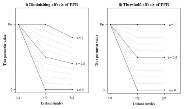
Regression parameter values used in simulations for i) diminishing and ii) threshold effects of fast food restaurants at distance 1/4, 1/2, and 3/4 miles. True parameter settings are β₁₂ = aβ₁₁ at 1/2 mile, β₁₃ = 0.8 aβ₁₁ at 3/4 mile for diminishing effects and β₁₂ = aβ₁₁ at 1/2 mile, β₁₃ = aβ₁₁ at 3/4 mile for threshold effects, such that a (0 ≤ a ≤ 1) controls the differences across parameters.

Note that, given the observed variances of the predictors (Table I), these effects constrain the marginal covariances between predictors and outcome to ${\sigma }_{X_{1}Y}={\beta }_{11}{\sigma }_{X_1}^2=0.011,{\sigma }_{X_{2}Y}=a{\beta }_{11}{\sigma }_{X_2}^2$, and ${\sigma }_{X_{3}Y}=a{\beta }_{11}{\sigma }_{X_3}^2$ for threshold effects, and ${\sigma }_{X_{3}Y}=0.8a{\beta }_{11}{\sigma }_{X_3}^2$ for diminishing effects. Further, we assumed the marginal outcome mean was μ_Y = 0 (centered) and had marginal variance ${\sigma }_Y^2=0.14$ (as observed in our motivating data).

To simulate outcomes, we first generated cluster-level values from a normal distribution with mean E [Ȳ_·j | FFR_1j;, FFR_2j, FFR_3j] = γ₀ + γ₁ FFR_1j + γ₂ FFR_2j + γ₃ FFR_3j and variance $\mathit{Var}[\overline{Y}{.}_j\mid {\mathit{FFR}}_{1j},{\mathit{FFR}}_{2j},{\mathit{FFR}}_{3j}]={\sigma }_{\delta }^2({\sigma }_{\delta }^2={\sigma }_Y^2-{\gamma }_1^2\mathit{Var}({\mathit{FFR}}_{1j})-{\gamma }_2^2\mathit{Var}({\mathit{FFR}}_{2j})-{\gamma }_3^2\mathit{Var}({\mathit{FFR}}_{3j})-2{\gamma }_1{\gamma }_2\mathit{Cov}({\mathit{FFR}}_{1j},{\mathit{FFR}}_{2j})-2{\gamma }_2{\gamma }_3\mathit{Cov}({\mathit{FFR}}_{2j},{\mathit{FFR}}_{3j})-2{\gamma }_3{\gamma }_1\mathit{Cov}({\mathit{FFR}}_{3j},{\mathit{FFR}}_{1j}))$. The conditional mean of the cluster level given all three predictors was used because the outcome needs to be simulated only once given all three predictors. We used the Sweep operator [10, 11] to derive conditional associations, γ₀, γ₁, γ₂, γ₃, given the specified marginal associations β₁₁, β₁₂, β₁₃ (see Appendix B). Given the cluster mean, we generated subject-level observations as Y_ij = Ȳ_·j + ∈_ij, where ${\epsilon }_{ij}~N(0,{\sigma }_{\epsilon }^2),{\sigma }_{\epsilon }^2=\frac{1-{\rho }_y}{{\rho }_y}{\sigma }_{\delta }^2$, and ρ_y = Corr (Y_ij,Y_{i′ j}) set to 0.05 for i ≠ i′ in the j^th cluster. With this parameter setting, the true marginal covariance matrix for the HMIM (11) has non-equal blocks (see Appendix C).

4.2. Simulation results

Let β̂_Ex denote the estimator for β in (12) when using V_kj = φ_k R_kj as the diagonal blocks of V_j (11), with R_kj being an exchangeable correlation structure with parameter ρ_k, k = 1, 2, 3. Similarly, let β̂_I denote the estimator for β when V_j consists of blocks of V_kj = φ_k R_kj with R_kj being the independence correlation structure. From the 1000 datasets, the empirical power was calculated as the rate of rejecting the overall test for comparing marginal effects β_1k for k = 1, 2, 3, i.e., H₀ : β₁₁ = β₁₂ = β₁₃ versus H₁ : at least one differs, for both estimators. For a given data set, the null hypothesis was rejected when the Wald test statistic T (Section 3.2) exceeded the critical value for a chi-squared distribution with 2 DOF. As shown in Figure 2, the empirical power of β̂_Ex was uniformly higher than β̂_I for diminishing effects of FFR. Power was always greater than the significance level (0.05) because in the range of a (0 ≤ a ≤ 1), true parameters of FFR were always distinguishable. The U-shape of the power function within the range of a is due to the non-centrality parameter of the test statistic, T, being a quadratic function of a under the alternative hypothesis.

Figure 2.

Simulation results assessing power for the hypothesis test H₀ : β₁₁ = β₁₂ = β₁₃ for i) diminishing and ii) threshold effects of fast food restaurants using hierarchical multiple informants model with exchangeable (Ex.) and independence (Indep.) correlation structures. True parameter settings are β₁₂ = aβ₁₁, β₁₃ = 0.8 aβ₁₁ for diminishing effects and β₁₂ = aβ₁₁, β₁₃ = aβ₁₁ for threshold effects.

For the threshold effects of FFR, the empirical powers of both estimators β̂_Ex and β̂_I go to nominal value (0.05) of Type I error rate when a = 1, or β₁₁ = β₁₂ = β₁₃. When β_1k’s are distinguishable or a goes to 0, the power for β̂_Ex increases faster than for β̂_I. The crossing of the power curves of the estimators may be due to Monte Carlo errors from the simulation. The Monte Carlo errors will be negligible with an increased number of simulations.

Because of the large number of clusters, the empirical power from the overall test when H₀ : β₁₁ = β₁₂ = β₁₃ is true preserved 5% Type I error rate. When the number of clusters is small, a bias corrected sandwich estimator could be used [12].

4.3. Simulation conclusions

Accounting for correlation within clusters is important to better detect small differences between marginal effects in an environmental study of clustered or hierarchical data. For instance, for threshold and diminishing effects, this simulation shows that, if using β̂_Ex 80% power was achieved when a < 0.2. That is, to be statistically distinguishable, the association between the outcome and number of FFR at the outer buffers needs to be at most 20% of the association with the number of FFR in the inner buffer. However, note that if using β̂_I, 80% power could not be reached for any value of a.

The fact that power using β̂_Ex is higher than β̂_I can be explained by applying previous work on asymptotic relative efficiency (ARE) of Mancl and Leroux [9]. According to their formula for ARE and given that we have the conditions: (i) invariant covariates within clusters, (ii) unequal cluster sizes (CV ≈ 1.1), (ii) large cluster size (J̄ = 145.6), and (iv) intra-cluster correlation ρ_k ≈ 0.05, k = 1, 2, 3, the ARE of β̂_Ex to β̂_I in the current data is about 0.55, meaning approximately 45% loss of efficiency by employing the independence correlation structure even for small intra-cluster correlation and invariant covariates within clusters.

This simulation study shows that an HMIM should be employed for formal testing of associations of an outcome among correlated predictors in clustered or hierarchical data to increase power.

5. Data example

We used data for children who participated in the 2007 California physical fitness test (also known as FitnessGram), which contains direct measures of children’s weight and height, among all children attending 5^th, 7^th, and 9^th grade, as well as other covariates such as age, sex, and race. Following prior exclusion criteria, we used data on 926,018 children nested in 6,323 schools [13]. The location of FFR and CS in California was purchased from InfoUSA, a commercial source. Geocodes for schools and food stores were cross-referenced to obtain the counts of stores within 1/4, 1/2, and 3/4 mile of a school, denoted by FFR₁, FFR₂, FFR₃ and CS₁, CS₂, CS₃. We obtained data from the California Department of Education’s databases, and the 2000 US Census to characterize the size and composition of the schools, as well as the socio-economic conditions of the neighborhoods in which schools were located.

Body mass index z-score was used as a continuous outcome. BMIz was derived by calculating body mass index (weight in kg/height in meters squared) and standardizing it according to an age and gender-specific BMI distribution. In other words, BMIz indicates how much a child’s BMI differs from a reference group of the same age and gender [14]. In contrast to BMI among adults, BMI among children needs to be standardized to a reference population because they are still growing and their body composition is changing as they grow [15] such that the meaning of BMI is not the same across age and sex. Following prior analyses [13], we included individual-level and school-level covariates as adjustment factors in models. The individual-level covariates are grade, age, gender, and race/ethnicity. The school-level covariates are school’s racial composition, school’s neighborhood-level education, school’s total enrollment, and percent of children enrolled in the free or reduced price meal program.

Descriptive statistics of child’s BMIz, the number of FFR and CS within distance 1/4, 1/2, and 3/4 miles are summarized in Table I. The average number of children per school and its standard deviation are 145.6 and 159.5, respectively, yielding the CV of 1.1.

We conducted two sets of analyses: (i) the comparison of two different features of food stores within the same buffer, and (ii) the comparison of a food environment feature across several buffer sizes. In both sets of analyses, we fitted an HMIM with both exchangeable and independence structures, and, for comparison, also MIM without accounting for cluster correlation. Further, the individual-level and school-level covariates described previously were included.

First, for the comparison of two different features of food stores within the same buffer, the counts of FFR and CS were standardized to a mean of zero and a standard deviation of one because of potentially different scales (e.g., an overall preponderance of one feature may be different compared with the other) so that the coefficients are in standard deviation units. We use $F_{1j}^s,F_{2j}^s,F_{3j}^s$ and $C_{1j}^s,C_{2j}^s,C_{3j}^s$ to denote the standardized number of FFR and CS within 1/4, 1/2, and 3/4 miles from the j^th school, respectively, and ${\mathit{Z}}_{ij}^T$ to denote the vector of the individual-level and the school-level covariates or confounders. For each of three buffers, k = 1, 2, 3, the fitted models are

$$\begin{array}{l}E[{\mathit{BMIz}}_{ij}\mid F_{kj}^s,{\mathit{Z}}_{ij}]={\beta }_{0k}^{F^s}+{\beta }_{1k}^{F^s}{F}_{kj}^s+{\mathit{Z}}_{ij}^T{\mathit{\beta }}_{(k)}^{F^s},\\ E[{\mathit{BMIz}}_{ij}\mid C_{kj}^s,{\mathit{Z}}_{ij}]={\beta }_{0k}^{C^s}+{\beta }_{1k}^{C^s}{C}_{kj}^s+{\mathit{Z}}_{ij}^T{\mathit{\beta }}_{(k)}^{c^s}.\end{array}$$

The null hypotheses of interest are whether for each buffer, the association between the number of CS and BMIz is the same as the association between the number of FFR and BMIz, i.e., $H_0:{\beta }_{1k}^{F^s}={\beta }_{1k}^{C^s}$ for k = 1, 2, 3.

Table II provides the results for the comparison of FFR and CS within the same buffer size. For all buffer sizes, the adjusted associations of CS with BMIz are significantly greater than those of FFR with BMIz. For example, given the 1/4 mile buffer size, child’s BMIz increases 0.77 × 10⁻³ and 10.82 × 10⁻³ per one standard deviation increase of FFR (= 0.679) and CS (= 0.473), respectively, after adjusting for individual and school factors. Using either an exchangeable correlation structure or the independence structure, we reached the same substantive conclusion, although the point estimates are slightly different.

Table II.

Estimated associations^* of two different features of the food environment (fast food restaurants vs. convenience stores) within the same buffer on body mass index z-scores and hypotheses tests of equality of the associations.

Distance	Association* or test	HMIM
		Exchangeable		Independence		MIM
		Est.	(SE)	Est.	(SE)	Est.	(SE)
1/4 mile	Std. fast food $\left({\beta }_{11}^{F^s}\right)$	0.77	(2.54)	−0.11	(2.33)	−0.11	(0.99)
	Std. convenience stores $\left({\beta }_{11}^{C^s}\right)$	10.82	(2.44)	7.78	(2.40)	7.78	(1.12)
	$H_0:{\beta }_{11}^{F^s}={\beta }_{11}^{C^s}$	P = 0.001		P = 0.009		P < 0.0001
1/2 mile	Std. fast food $\left({\beta }_{12}^{F^s}\right)$	1.96	(3.46)	2.75	(2.66)	2 75	(1.10)
	Std. convenience stores $\left({\beta }_{12}^{C^s}\right)$	11.56	(2.88)	10.35	(2.72)	10.35	(1.14)
	$H_0:{\beta }_{12}^{F^s}={\beta }_{12}^{C^s}$	P = 0.003		P = 0.009		P < 0.0001
3/4 mile	Std. fast food $\left({\beta }_{13}^{F^s}\right)$	5.02	(3.36)	5.59	(2.73)	5.59	(1.15)
	Std. convenience stores $\left({\beta }_{13}^{C^s}\right)$	13.24	(3.00)	13.80	(2.82)	13.80	(1.18)
	$H_0:{\beta }_{13}^{F^s}={\beta }_{13}^{C^s}$	P = 0.005		P = 0.004		P < 0.0001

Associations are estimated on the basis of standardized number of fast food restaurants and convenience stores, adjusting for individual-level and school-level covariates, using the proposed hierarchical multiple informants model and the multiple informants model without accounting for within cluster correlation.

^*Estimate and SE were multiplied by 10³ to enhance readability.

Second, to investigate how the association between the number of FFR (or CS) and BMIz varies across several buffers, we fitted models $E[{\mathit{BMIz}}_{ij}\mid {\mathit{FFR}}_{kj},{\mathit{Z}}_{ij}]={\beta }_{0k}+{\beta }_{1k}{\mathit{FFR}}_{kj}+{\mathit{Z}}_{ij}^T{\mathit{\beta }}_{(k)}$ for k = 1, 2, 3 (similar for CS).

The question of interest is whether the associations between the number of a given foods store type (FFR or CS) varies across buffer sizes, i.e., the overall null hypothesis H₀ : β₁₁ = β₁₂ = β₁₃. Note that the coefficients are expressed in units of BMIz per one unit increase in the number of stores, because the same feature is being compared across buffers. The parameter estimates and the p-values for the overall hypotheses tests are given in Table III.

Table III.

Estimated associations^* between number of fast food restaurants (or convenience stores) and body mass index z-scores across three distances and test of equality of association across distances.

Distance	Association* or Test	HMIM
		Exchangeable		Independence		MIM
		Est	(SE)	Est	(SE)	Est	(SE)
1/4 mile	Fast Food (β11)	1.14	(3.73)	−0.17	(3.21)	−0.17	(1.36)
1/2 mile	Fast Food (β12)	1.12	(1.97)	1.56	(1.42)	1.56	(0.59)
3/4 mile	Fast Food (β13)	1.72	(1.15)	1.92	(0.88)	1.92	(0.37)
	H0 : β11 = β12 = β13	P = 0.895		P = 0.782		P = 0.265
1/4 mile	Convenience store (β11)	22.89	(5.16)	16.47	(4.77)	16.47	(2.23)
1/2 mile	Convenience store (β12)	10.67	(2.66)	9.55	(2.36)	9.55	(0.99)
3/4 mile	Convenience store (β13)	7.17	(1.62)	7.48	(1.44)	7.48	(0.60)
	H0 : β11 = β12 = β13	P = 0.004		P = 0.118		P = < 0.001

Associations are estimated from three different models, adjusting for individual-level and school-level covariates.

^*Estimate and SE was multiplied by 103 to enhance readability

The overall test for the associations of FFR across several buffers is not rejected (p = 0.895), meaning the number of FFR within 1/4, 1/2, and 3/4 mile from a school do not have significantly different associations with child’s BMIz. This implies that the most relevant buffer size is 3/4 mile from a school, or potentially further. Child’s BMIz increases 1.72 × 10⁻³ per one FFR increment within 3/4 miles from a school (p = 0.862, not reported in Table III). By employing either an exchangeable correlation matrix or the independence structure, the same conclusion is derived.

Unlike the associations of FFR, the associations of CS across the buffers are significantly different based on HMIM with the exchangeable correlation matrix (p = 0.004). On the basis of the result of HMIM with the exchangeable correlation matrix, we performed subsequent hypothesis test as described in Section 3.2. i.e., test the one-sided null hypothesis, H₀ : β₁₁ ≤ β₁₂. We rejected the one-sided null hypothesis (p = 0.017) and concluded that the most relevant buffer size for the association between CS and child’s BMIz is 1/4 mile from a school. Child’s BMIz increases 0.022 per one CS increment within 1/4 miles from a school after adjusting other covariates.

Note that in Tables II and III, the estimates and standard errors using an exchangeable correlation matrix differ from those using the independence assumption. These changes result in test statistics (e.g., a ratio of the difference between two regression parameters to its standard error) that are larger when using the exchangeable correlation matrix and thus smaller p-values. For instance, in Table III the overall null hypothesis yields a p-value = 0.118 when using the independence assumption within cluster while an exchangeable assumption yielded a p–value = 0.004, highlighting the gain in efficiency when using the exchangeable versus independence assumption.

Lastly, as shown in Tables II and Table III, the MIM without accounting for within-cluster correlation provides the same point estimates of HMIM with the independence structure, but the failure to account for hierarchical structures yields the underestimated standard errors, resulting in invalid inference.

6. Discussion

We extended multiple informants methods to a hierarchical data setting to enable comparison of the associations between multiple correlated predictors on a univariate outcome measured in clustered sets of individuals. The method is based on a non-standard application of generalized estimating equations and can be applied to settings where the outcome is continuous, count, or binary. In the simulation study, we showed the improved power and efficiency of estimators based on using a block diagonal of exchangeable correlation matrices instead of the working independence correlation structure. A practical advantage of an HMIM is that it can be fitted using available GEE software. A marginal GEE model for each multiple informant can be separately fitted, and then a joint empirical variance estimator can be calculated to conduct hypothesis tests involving the marginal effects of predictors. We applied HMIMs to examine how the association between the number of FRR (or CS) and child’s BMIz varies across several buffers from a school and to compare the association of two different features of the food environment (FFR vs. CS) with child’s BMIz. The overall hypothesis that the association between number of FFR and child’s BMIz across several buffers is the same was not rejected, suggesting that the association of the count of FFR up to 3/4 mile from a school does not differ significantly from the association at small buffer sizes with accounting for individual-level and school-level covariates. In contrast, the association of BMIz with the count of CS differs depending on distance from a school, with 1/4 mile being most relevant buffer size. We also showed the association between the count of CS and BMIz is much stronger compared with the association between FFR and BMIz.

We proposed a testing strategy that may be helpful in selecting an appropriate buffer size at which to estimate the association between an environmental feature and an outcome. However, there are some extreme cases where the hypothesis testing strategy may fail. For instance, if there are few or no additional of food stores between distances d_{k − 1} and d_k, then the marginal association between the number of food stores and child’s BMIz across buffers d_{k − 1} and d_k would likely to be the same due to X_{k − 1, j} ≈ X_kj. An alternative might be to define multiple informant covariates as the new information not contained in the previous buffer, e.g., X_j (δ_k) = X_kj − X_{k − 1, j}, and fit a model $g({\mu }_{ij})={\beta }_0^{\ast }+{\beta }_1^{\ast }{X}_j({\delta }_1)+{\beta }_2^{\ast }{X}_j({\delta }_2)+{\beta }_3^{\ast }{X}_j({\delta }_3)$. If ${\beta }_3^{\ast }\ne 0$, then the buffer of size is d₃ from a school still provides information on child’s BMIz, and similarly for the other buffer sizes. However, the interpretation of these coefficients is that of conditional associations, not marginal associations.

We also confirmed the underestimated variances of the estimators from the MIM because of the failure to incorporate hierarchical structures, which provide us invalid inference. The bootstrap method, as pointed out by a referee, may be employed for valid inference. For instance, suppose that we have 5000 bootstrap estimates of regression parameters from the MIM. Then, the empirical variance/covariance of the estimates can be used for hypothesis testing because the failure to account for hierarchical structures has little impact on the population point parameter estimates. The bootstrap method, however, may require extensive computational time.

The main idea of MIM is very similar to seemingly unrelated regression methods (SUR) [16]. The main difference between MIM and SUR is that in MIM the same outcome is replicated to form an outcome vector for the cluster with predictors changing from one replicate to another, whereas different outcomes form an outcome vector in SUR. Similarly, an HMIM is related to the model structure described by Rochon [17]. The author employed SUR in a repeated measures setting for discrete and continuous outcome variables; nevertheless, here we extended MIM to hierarchical data to enable estimation and testing of marginal effects of several correlated factors or multiple informants or predictors.

Possible extensions of this work may include estimating non-linear or semi-parametric associations between multiple predictors and outcomes (e.g., penalized splines). Furthermore, the size of the buffer may vary by whether schools are located in urban or rural locations, or other spatially varying features of the environment. Hence, a future area of research can be to investigate the spatial variation of the coefficients and/or tests presented in the present article.

The methods presented are motivated by school environment contributions to childhood obesity, yet such methods apply more broadly to other environmental features and other types of nested outcome data. For example, the proposed approach can be applied to study questions concerning the relative influence of home versus work environment on adult health outcomes such as cardiovascular disease or quality of life.

References

- 1.Davis B, Carpenter C. Proximity of fast-food restaurants to schools and adolescent obesity. American Journal of Public Health. 2009;99(3):505–510. doi: 10.2105/AJPH.2008.137638. [DOI] [PMC free article] [PubMed] [Google Scholar]
- 2.Horton NJ, Laird NM, Zahner GEP. Use of multiple informant data as a predictor in psychiatric epidemiology. International Journal of Methods in Psychiatric Research. 1999;8(1):6–18. [Google Scholar]
- 3.Pepe MS, Whitaker RC, Seidel K. Estimating and comparing univariate associations with application to the prediction of adult obesity. Statistics in Medicine. 1999;18(2):163–173. doi: 10.1002/(sici)1097-0258(19990130)18:2<163::aid-sim11>3.0.co;2-f. [DOI] [PubMed] [Google Scholar]
- 4.Horton NJ, Fitzmaurice GM. Regression analysis of multiple source and multiple informant data from complex survey samples. Statistics in Medicine. 2004;23(18):2911–2933. doi: 10.1002/sim.1879. [DOI] [PubMed] [Google Scholar]
- 5.Litman HJ, Horton NJ, Hernández B, Laird NM. Estimation of marginal regression models with multiple source predictors. Handbook of Statistics. 2008;27(7):730–746. doi: 10.1002/sim.2593. [DOI] [PMC free article] [PubMed] [Google Scholar]
- 6.Liang KY, Zeger SL. Longitudinal data analysis using generalized linear models. Biometrika. 1986;73(1):13–22. [Google Scholar]
- 7.Pan W, Louis TA, Connett JE, Connett E. A note on marginal linear regression with correlated response data. The American Statistician. 2000;54(3):191–195. [Google Scholar]
- 8.Sullivan PM, Anderson GL. A cautionary note on inference for marginal regression models with longitudinal data and general correlated response data. Communications in Statistics. 1994;23(4):939–951. [Google Scholar]
- 9.Mancl LA, Leroux BG. Efficiency of regression estimates for clustered data. Biometrics. 1996;52(2):500–511. [PubMed] [Google Scholar]
- 10.Beaton AE. Research Bulletin RB–64–51. Princeton, NJ: 1964. The use of special matrix operators in statistical calculus. [Google Scholar]
- 11.Dempster AP. Elements of Continuous Multivariate Analysis. Addison-Wesley; Reading, MA: 1969. [Google Scholar]
- 12.Mancl LA, Derouen TA. A covariance estimator for GEE with improved small-sample properties. Biometrics. 2001;57:126–134. doi: 10.1111/j.0006-341x.2001.00126.x. [DOI] [PubMed] [Google Scholar]
- 13.Sánchez BN, Sanchez-Vaznaugh EV, Uscilka A, Baek J, Zhang L. Differential associations between the food environment near schools and childhood overweight across race/ethnicity, gender, and grade. American Journal of Epidemiology. 2012;175(12):1284–1293. doi: 10.1093/aje/kwr454. [DOI] [PMC free article] [PubMed] [Google Scholar]
- 14.Centers for Disease Control and Prevention. CDC growth charts, United States. Atlanta (GA): CDC; 2005. Retrieved January 28, 2010, from http://www.cdc.gov/GROWTHcharts/ [Google Scholar]
- 15.Must A, Anderson SE. Body mass index in children and adolescents: considerations for population-based applications. International Journal of Obesity. 2006;30(4):590–594. doi: 10.1038/sj.ijo.0803300. [DOI] [PubMed] [Google Scholar]
- 16.Zellner A. An efficient method of estimating seemingly unrelated regressions and tests for aggregation bias. Journal of the American Statistical Association. 1962;57(298):348–368. [Google Scholar]
- 17.Rochon J. Analyzing bivariate repeated measures for discrete and continuous outcome variables. Biometrics. 1996;52(2):740–750. [PubMed] [Google Scholar]
Associated Data
This section collects any data citations, data availability statements, or supplementary materials included in this article.