A simple molecular mechanics integrator in mixed rigid body and dihedral angle space

Abstract

We propose a numerical scheme to integrate equations of motion in a mixed space of rigid-body and dihedral angle coordinates. The focus of the presentation is biomolecular systems and the framework is applicable to polymers with tree-like topology. By approximating the effective mass matrix as diagonal and lumping all bias torques into the time dependencies of the diagonal elements, we take advantage of the formal decoupling of individual equations of motion. We impose energy conservation independently for every degree of freedom and this is used to derive a numerical integration scheme. The cost of all auxiliary operations is linear in the number of atoms. By coupling the scheme to one of two popular thermostats, we extend the method to sample constant temperature ensembles. We demonstrate that the integrator of choice yields satisfactory stability and is free of mass-metric tensor artifacts, which is expected by construction of the algorithm. Two fundamentally different systems, viz., liquid water and an α-helical peptide in a continuum solvent are used to establish the applicability of our method to a wide range of problems. The resultant constant temperature ensembles are shown to be thermodynamically accurate. The latter relies on detailed, quantitative comparisons to data from reference sampling schemes operating on exactly the same sets of degrees of freedom.

I. INTRODUCTION

Molecular mechanics is the classical description of the internal and relative motions of molecules using suitable interaction potentials known as force fields. These models have been explored most often by the numerical integration of Newton's equations of motion, i.e., by molecular dynamics (MD).¹ Auxiliary constructs couple the system to an external bath (thermostats and manostats), and these methods are often required to generate data that can be compared to experiment. Thermodynamic information is obtained in much more straightforward ways from these simulations than dynamical information. The reasons lie in the focus of parameterization of the models toward thermodynamics, in the greater dependence of measured dynamics on details of the simulation setup,² and in the different susceptibilities to discretization error.³

The statistical precision of data obtained by unbiased molecular dynamics methods depends primarily on simulation length.⁴ This motivates ongoing optimization and development on software and hardware levels.^5,6 The cost of molecular mechanics is dominated by the evaluation of forces and it is desirable to maximize the simulation time between successive evaluations. However, increases in the integration time step (δt) lead to increasing discretization errors, which bias results and eventually lead to catastrophic instability.^3,7 In the canonical ensemble, integrator errors are absorbed by the thermostat. This leads to incorrect averages and fluctuations of thermal variables and can alter the equipartition of kinetic energy amongst degrees of freedom.^8,9 Discretization errors are amplified for particles with low mass subjected to stiff potentials. Consequently, much work has focused on algorithms that address the stability issue either by redistributing or changing atomic masses¹⁰ or by eliminating the fastest motions altogether (constrained dynamics). Geometric constraints can be incorporated via techniques based on Lagrange multipliers coupled to approximate or iterative solvers¹¹ and techniques resorting explicitly to generalized coordinate spaces.¹² This paper is concerned with an approach to the latter.

Given the difficulty in defining “correct,” thermostatted dynamics,⁷ it seems justifiable to mandate that molecular simulations should first and foremost yield accurate and statistically robust information regarding the equilibrium configurational distributions. Accordingly, a wide spectrum of methods has emerged whose focus it is to explore the multidimensional energy landscape governed by the force field of interest.¹³ These approaches, often by design, sacrifice the pursuit of dynamical information in favor of extracting thermodynamic quantities. The most extreme realization of this is the use of a random Monte Carlo (MC) propagator capable of sampling different amplitudes of motions in a manner that is even specific to individual degrees of freedom.¹⁴

Unfortunately, the inclusion of constraints can rarely be decoupled from force field parameterization. This means that simulations incorporating a significant deviation from the set of constraints used during parameterization will produce inconsistent equilibrium statistics.^15,16 While the most common biomolecular force fields assume, at most, constrained bond lengths, there are a few important models that assume dihedral angles as the only internal degrees of freedom, for example, ECEPP¹⁷ or ABSINTH.¹⁸ Most prominently, the ROSETTA paradigm generally keeps bond lengths and angles fixed, and this is reflected in its composite energy function.¹⁹ It is therefore of continued interest to have access to a stable molecular dynamics engine that efficiently produces unbiased equilibrium ensembles for force fields that use constant bond lengths and angles. This paper proposes one such method. For clarity, we first review the difficulties associated with designing a stable, efficient, and configurationally unbiased algorithm that uses torsional molecular dynamics to achieve an accurate description of equilibrium statistics in constant temperature ensembles.

Consider a system of N_at atoms organized into N_mol molecules each with position vectors ${\vec{r}}_i$ with i = 1, …, N_at. The vectors ${\vec{r}}_i$ are assumed to be in a space-fixed, global reference frame. Together, they constitute the state vector r of dimensionality 3N_at associated with this Cartesian coordinate space. We assume a separable Hamiltonian with a potential energy U(r), which is written explicitly or implicitly as a function of r such that any given conformation specified by r has a single, well-defined value for U. Using momenta and positions as independent variables (Hamiltonian formulation), the integration of the classical equations of motions takes the following form:

$$\begin{array}{c}\dot{\mathbf{p}}=-\nabla U\left(\mathbf{r}\right),\hfill \\ \dot{\mathbf{r}}={\mathbf{M}}^{-1}\mathbf{p}.\hfill \end{array}$$ (1)

The mass matrix M is diagonal and trivially inverted. Because the kinetic energy is $\frac{1}{2}{\mathbf{p}}^{\mathbf{T}}{\mathbf{M}}^{-\mathbf{1}}\mathbf{p}$ with M⁻¹ also being diagonal, there is no direct coupling between the 3N_at differential equations for $\dot{\mathbf{r}}$, and any correlation results indirectly from the particular functional form of U(r). It is possible to explicitly constrain any given coordinate by setting its momentum to zero without changing the contributions to the kinetic energy made by other degrees of freedom. This means that the factor resulting from integrating the momenta in the partition function is constant for a given set of constraints and temperature and independent of r.

In generalized coordinates ϕ of the same dimensionality (3N_at) the kinetic energy is written as $E_k=\frac{1}{2}{\mathbf{p}}_{\varphi }^{\mathbf{T}}{\left({\mathbf{J}}^{\mathbf{T}}\mathbf{MJ}\right)}^{-\mathbf{1}}{\mathbf{p}}_{\varphi }=\frac{1}{2}{\mathit{\omega }}^{\mathbf{T}}\left({\mathbf{J}}^{\mathbf{T}}\mathbf{MJ}\right)\mathit{\omega }$. The Jacobian matrix J describes the coordinate transformation from Cartesian to generalized coordinates and its elements are $J_{kl}=\frac{\delta r_k}{\delta {\varphi }_l}$. The p_ϕ are the generalized momenta conjugate to the generalized velocities, ω, i.e., p_ϕ = (J^TMJ)^{− 1}ω. The matrix G = J^TMJ is called the mass-metric tensor (MMT). For a separable Hamiltonian H(p_ϕ,ϕ) written as a sum of E_K(p_ϕ) and U(ϕ), the partition function in the canonical ensemble is Q = ∫exp [−βH(p_ϕ, ϕ)]dp_ϕdϕ. Here, we have used shorthand notation for the multidimensional integral, and β equals (k_BT)⁻¹, where k_B is Boltzmann's constant and T is the ensemble temperature. Integration over the generalized momenta yields $Q=\int \sqrt{\det \mathbf{G}}\exp \left[-\beta U\left(\mathit{\varphi }\right)\right]d\mathit{\varphi }$.²⁰ In the absence of any constraints on the degrees of freedom, the determinant of the MMT is independent of ϕ, and Q can be written as a product of thermal and configurational contributions: Q = Q_TQ_C = C(T)∫exp [−βU(ϕ)]dϕ.

The equations of motion for the generalized momenta become:

$${\dot{\mathbf{p}}}_{\varphi }=\frac{d}{dt}\left[\left({\mathbf{J}}^{\mathbf{T}}\mathbf{MJ}\right)\mathit{\omega }\right]=-\mathbf{J}\nabla U\left(\mathbf{r}\right)={\mathbf{F}}_{\varphi }.$$ (2)

In Eq. (2), we formally impose constraints by letting a subset of elements of ω be zero at all times. Conjugate momenta become zero as well, and the constrained coordinates are no longer integrated over. This leads to a term $\sqrt{\det {\mathbf{G}}_{\mathbf{S}}}$ in the configurational probability density of the free subsystem with det(G) ≠ det(G_S). More importantly, the constraints lead to the artifact whereby, unlike det(G), det(G_s) varies with ϕ (we refer to these effects as MMT artifacts), and this is highlighted in panel (a) of Fig. S1 in the supplementary material.²¹ The dependence on conformation derives from coupling terms between constrained and unconstrained coordinates in the expression for the kinetic energy and is zero only if the constrained coordinates correspond to a complete block in a block diagonal MMT (e.g., an entire molecule).

The magnitude of MMT artifacts depends on the level of coupling, and it can be argued that corrections for the weakly coupled constraints supported by linear solvers such as SHAKE²² are negligible (panel (e) in Fig. 1). Fixman advocated the use of compensating potentials containing det(G_S) explicitly to alleviate the statistical bias introduced by MMT artifacts. These corrections have been derived in different forms and shown to be effective,^20,23–26 yet they are not routinely in use. Numerical efficiency is an important consideration for algorithms meant to propagate ϕ directly. Many published algorithms scale unfavorably with system size either because one of the nondiagonal matrices is considered explicitly or because one requires second derivatives.^12,27

FIG. 1.

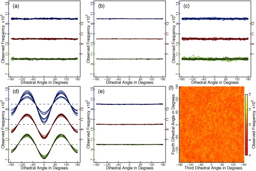
Absence of mass-metric tensor artifacts in simulations using Eq. (11) in the main text. (a) Histograms (100 bins) are plotted for all 15 dihedral angle degrees of freedom of the chain for 3 different mass distributions. Data sets are shifted to allow a more compact visualization within a single panel, and separate y-axes are provided (color coded). Red, green, and blue colors indicate the chosen distribution of masses (Sec. II E 1). Within each subset, colors change from light to dark in correspondence with the position of the dihedral angle along the chain. Dashed lines indicate the unbiased (flat) distributions we expect to observe. Data are for Eq. (11) with the Andersen thermostat and using the middle of the chain as the base of motion. (b) The same as (a) for the velocity rescaling thermostat. Note that individual velocities can never change sign due to the rescaling protocol (see Appendix C). (c) The same as (a) when using the first 3 atoms of the chain as the base of motion. (d) Results as in (a) are shown for a Cartesian Langevin integrator with bond length and angle constraints. (e) The same as (d) for simulations using just bond length constraints. (f) We plot a two-dimensional histogram for two specific dihedral angles. Data correspond to the conditions for the red data set in (a). Panels (a)–(c) and (f) establish the absence of MMT artifacts, which are clearly discernible in panel (d) and Fig. S1(a) in the supplementary material.²¹

An efficient treatment of complex constraints is made possible by formalisms originally developed in other fields.^28–30 Recursive computations of det(G_S) or its derivatives with ϕ have been established,^23,31 and these scale linearly with system size. By considering each molecule as a chain of rigid bodies connected by hinges³² with a base and at least one tip (branched chains have correspondingly more tips), the free subsystem comprises K degrees of freedom, which are a combination of torsional ones (hinges) and external ones (global motion of the base). It has been argued that generalized coordinates are rarely useful for molecular dynamics,³³ and the complexities encountered even for integrators for simple rigid bodies underline the value of the simple structure of Eq. (1).^34–36 Additionally, Eq. (2) reveals the existence of bias terms deriving from the time dependence of the generalized momenta that must now involve the time derivative of J. Elements of J for angular degrees of freedom are given by

$$\left(\begin{array}{ccc}{J}_{3i-2,k}& J_{3i-1,k}& J_{3i,k}\end{array}\right)=\frac{\partial {\vec{r}}_i}{\partial {\varphi }_k}={\vec{a}}_k\times \left({\vec{r}}_i-{\vec{b}}_k\right).$$ (3)

In Eq. (3), ${\vec{a}}_k$ is the respective unit length vector specifying the axis of rotation and ${\vec{b}}_k$ is a reference point on the axis. The time derivative of J produces torques not related to F_ϕ.^12,29,37 This is true irrespective of whether we introduce constraints to create the K-dimensional space defined above. The time dependence of J describes well-known effects observed in systems with multiple rotating frames. It has also been proposed that the use of fully flexible hinges will eliminate the need for bias terms.³⁵ Importantly, the variable transformation in Eq. (2) is canonical, and the resultant MMT artifacts must be compensated if constraints are in use.^23,26

The approach proposed in this paper is different in this regard. It neither ignores MMT artifacts nor corrects for them using a Fixman-style potential. We never evaluate det(G_S) or det(G) or its derivatives explicitly. Instead, we derive propagators for ϕ and ω that can be shown to correspond to a (generally) artificial dynamics on a modified constant energy hypersurface with ${\Omega }_k=I_{kk}^{1/2}{\omega }_k$ and ϕ_k as the underlying independent variables. Here, the I_kk are the diagonal elements of the MMT, and the modified kinetic energy is $E_k^{\prime }=\frac{1}{2}{\sum }_k^K{I}_{kk}{\omega }_k^2$. This restores Eq. (2) to the simple form of Eq. (1) while lumping all bias torques into a time dependence of effective masses. Given r and ∇U(r), the I_kk and F_ϕ are calculated recursively in linear time. We have coupled the integrator to two well-known thermostatting schemes to obtain constant temperature configurational statistics. Because the kinetic energy is modified, and because the level of dynamic coupling is reduced, the system dynamics are modified for all but special cases. This is precisely what allows the propagator to avoid MMT artifacts by construction. Simplicity, versatility, and most importantly thermodynamic correctness are our main design goals. We achieve these by sacrificing dynamical accuracy, and the method is therefore in the spirit of MC propagators.

The remainder of the text is organized as follows: First, we introduce our methodology for obtaining equilibrium sampling of the configurational distribution by propagating trajectories in a mixed torsional/rigid body space. We test integrator stability using long, flexible, self-avoiding chains as the benchmarking system. Detailed results are presented for two systems of relevant complexity that establish the thermodynamic accuracy of the sampling obtained using our approach. Tests of accuracy are achieved through comparisons to results obtained for the same two systems using a suitable MD integrator and an MC propagator, respectively.

II. METHODS

A. Motivation of approximations

In the development of the method, we focused on the following goals:

• 1.Avoiding MMT artifacts to make data comparable with those generated by MC simulations in the same coordinate space.³¹
• 2.Ease of implementation and computational efficiency: Auxiliary computations should scale as O(N_at) as in established approaches.^29,37
• 3.Stable numerical integration.
• 4.Seamless extension to simulations with multiple molecules. This is important because external motion does not seem to be a trivial issue in the most common framework.^38,39
• 5.Thermodynamic, but not kinetic correctness since the constraints themselves will usually make it difficult to assign physical meaning to the apparent dynamics of a molecular system.

Using the same notation as above, we follow the approach of representing the system in a set of mixed rigid-body and dihedral angle coordinates of overall dimensionality K ⩽ N_at. The dihedral angles are a subset of a typical molecular Z matrix, i.e., a set of M − 1 bond lengths, M − 2 bond angles, and M − 3 dihedral angles defined for atoms separated by 1, 2, and 3 covalent bonds, respectively. Except for the first 3 atoms, each of the M atoms in a molecule has one associated coordinate of each type. All bond lengths and angles and some dihedral angles correspond to constraints. The rigid-body coordinates of the N_mol molecules are encoded by using Cartesian coordinates for the first three atoms in each molecule (Appendix A). For this choice, we stipulate a reversible mapping:

$$\varphi =A\left(\mathbf{r}\right)\mathrm{and}\mathbf{r}=A^{-1}\left(\varphi \right).$$ (4)

Here, A is the nonlinear operator encompassing all the functions needed for the coordinate transformation and A⁻¹ is its inverse. We impose a tree-like structure for the operator A⁻¹, which means that a molecule is built from its first three atoms onward using Z matrix variables³⁷ while imposing an arbitrary directionality and full backward dependency along the main chain and a backward dependency to the branch point for branches (such as polypeptide side chains). The choice of Z matrix-like variables is based on convenience but poses limitations for systems with flexible rings. This is because one of the ring bonds is not represented in the Z matrix and cannot be constrained explicitly. It has been argued that these variables are generally far from optimal,¹² but we use them here because more informative coordinates of universal merit across multiple conditions (like temperature) cannot be identified without prior knowledge for systems with high conformational flexibility.

The key approximation of our approach is to now stipulate a diagonal mass matrix such that

$$E_k^{\prime }=\frac{1}{2}{\sum }_i^K{I}_{ii}{\omega }_i^2=\frac{1}{2}{\mathit{\omega }}^{\mathbf{T}}{\mathbf{I}}_D\mathit{\omega }\ne \frac{1}{2}{\mathbf{p}}^{\mathbf{T}}{\mathbf{M}}^{-\mathbf{1}}\mathbf{p}.$$ (5)

Here, the approximate kinetic energy is obtained from the stipulated diagonal mass matrix I_D and the generalized velocities, and it will in general be different from the standard kinetic energy as used above. This approximation is an important step toward satisfying point 1 above, because the kinetic coupling is explicitly removed. This of course comes at the cost of having introduced a potentially severe approximation – an issue that we address in detail below. The diagonal matrix implies that structurally the problem becomes very similar to that in unconstrained Cartesian dynamics, i.e., equations of motion are formally decoupled. This restores important notions such as the equipartition principle to their intuitive forms.⁴⁰ Note that units across the elements in ϕ are heterogeneous, which is relevant for both forces and effective masses. Effective masses correspond to the appropriate masses and rotational inertia for linear and angular motion, respectively:

$$\begin{array}{c}\hfill \mathrm{diag}\left({\mathbf{I}}_D\right)=\left[\begin{array}{ccc}\begin{array}{ccc}{M}^1& M^1& M^1\end{array}& \begin{array}{ccc}{I}_x^1& I_y^1& I_z^1\end{array}& \begin{array}{ccc}{I}_{\varphi 1}^1& ...& \begin{array}{ccc}{I}_{\varphi k}^1& M^2& ...\end{array}\end{array}\end{array}\right].\end{array}$$ (6)

In Eq. (6), upper indices denote which molecule the degrees of freedom belong to, M denotes molecular mass, I_x/y/z represent rotational inertia around axes defined by the base vectors of the global reference frame passing through the molecular center of mass, and the I_ϕi denote effective masses (inertia) for rotation around the ith dihedral angle in that molecule. The elements of I_D, which we refer to as I_kk throughout, as well as F_ϕ⁴¹ and estimates for $\dot{\mathbf{r}}$ can all be obtained by the recursive computations provided as Eqs. (B1)–(B3).

B. Numerical integration scheme on a constant energy hypersurface

We derive a numerical scheme by mandating conservation of energy, $E_k^{\prime }\left(\mathit{\omega }\right)+U\left(\mathbf{r}\right)$, for a discrete integration step t₁ → t₂:

$$\begin{array}{ccc}\hfill 0& =& \frac{1}{2}\left[\mathit{\omega }{\left(t_2\right)}^{\mathbf{T}}{\mathbf{I}}_{\mathbf{D}}\left(t_2\right)\mathit{\omega }\left(t_2\right)-\mathit{\omega }{\left(t_1\right)}^{\mathbf{T}}{\mathbf{I}}_{\mathbf{D}}\left(t_1\right)\mathit{\omega }\left(t_1\right)\right]\hfill \\ & & +U\left(t_2\right)-U\left(t_1\right),\hfill \\ \\ \hfill 0& =& \mathit{\omega }{\left(t_2\right)}^{\mathbf{T}}{\mathbf{I}}_{\mathbf{D}}\left(t_2\right)\mathit{\omega }\left(t_2\right)-\mathit{\omega }{\left(t_1\right)}^{\mathbf{T}}{\mathbf{I}}_{\mathbf{D}}\left(t_1\right)\mathit{\omega }\left(t_1\right)\hfill \\ & & -\delta t\left(\mathit{\omega }\left(t_1\right)+\mathit{\omega }\left(t_2\right)\right){\mathbf{F}}_{\varphi }\left(t_{1.5}\right).\hfill \end{array}$$ (7)

This single condition is not sufficient to constrain the dynamics meaningfully. However, because of the diagonal nature of I_D and in analogy to the Cartesian case, it is reasonable to mandate that Eq. (7) be fulfilled by each of the K degrees of freedom independently:

$$\begin{array}{ccc}& & {\omega }_k{\left(t_2\right)}^2-I_{kk}{\left(t_2\right)}^{-1}[\delta t\left({\omega }_k\left(t_2\right)+{\omega }_k\left(t_1\right)\right)F_{\varphi ,k}\left(t_{1.5}\right)+I_{kk}\left(t_1\right){\omega }_k{\left(t_1\right)}^2]=0\hfill \\ & & \\ & & {\omega }_k\left(t_2\right)=\delta t\frac{F_{\varphi ,k}\left(t_{1.5}\right)}{2I_{kk}\left(t_2\right)}\hfill \\ & & \pm \frac{\sqrt{F_{\varphi ,k}{\left(t_{1.5}\right)}^2\delta t^2+4I_{kk}\left(t_2\right){\omega }_k\left(t_1\right)F_{\varphi ,k}\left(t_{1.5}\right)\delta t+4I_{kk}\left(t_2\right)I_{kk}\left(t_1\right){\omega }_k{\left(t_1\right)}^2}}{2I_{kk}\left(t_2\right)}.\hfill \end{array}$$ (8)

Equations (7) and (8) contain a time dependence of I_kk that is meant to preserve kinetic energy for angular variables in the diagonal assumption. This is fundamentally different from the way the aforementioned bias torques would steer the system toward preserving both total angular momentum and the correct total energy in the context of a nondiagonal mass matrix. As a result, the level of dynamical coupling and the overall system dynamics are altered. Note that the initial choices for ω define the hypersurface explored by the new dynamics.

Equation (8) is time-reversible, which, in a weak sense, is a desirable property.⁷ However, Eq. (8) is not guaranteed to have a real solution, and we address this as follows. We can approximate I_kk(t₂) in the second term in the square root by $\sqrt{I_{kk}\left(t_1\right)I_{kk}\left(t_2\right)}$. Then, only one of the solutions to the quadratic equation is meaningful:

$${\omega }_k\left(t_2\right)\approx \delta t\frac{F_{\varphi ,k}\left(t_{1.5}\right)}{I_{kk}\left(t_2\right)}+\sqrt{\frac{I_{kk}\left(t_1\right)}{I_{kk}\left(t_2\right)}}{\omega }_k\left(t_1\right).$$ (9)

In practice, we use Eq. (9), which is not time-reversible, as a guide to identify the correct solution for Eq. (8). All integrators presented in this paper use the simplest update rule for ϕ:

$${\varphi }_k\left(t_{2.5}\right)={\varphi }_k\left(t_{1.5}\right)+\delta t{\omega }_k\left(t_2\right).$$ (10)

The only exception to Eq. (10) is rigid-body rotation, for which we directly construct a quaternion from the ω_k(t₂), i.e., there is no explicit representation of the corresponding ϕ_k (see below).

Equation (8) is also implicit because the I_kk(t₂) are needed to determine the new angular velocities. We use the assumed time dependence I_kk(t) to mask the true dependence I_kk({ϕ_{j ≠ k}(t)}). Consequently, the required values for I_kk(t₂) are obtained by guessing the values for ϕ_k(t₂) and not by extrapolating the apparent time dependencies of the I_kk themselves. In detail, we first obtain a guess of all relevant ω_k(t_1.5) using Eq. (8) with t₂ replaced with t_1.5 throughout and δt/2 instead of δt. This is followed by a positional increment by δt/2 to advance the ϕ_k(t_1.5) to ϕ_k(t₂) similar to Eq. (10). The impact of the underlying asymmetry (the deterministic force uses the values obtained for t_1.5 and not for t_1.75) is weakened by the fact that the new conformation is used exclusively to calculate guesses for the I_kk(t₂). Upon restoring the system configuration to that encoded by ϕ_k(t_1.5), Eq. (8) is applied as written. The resultant scheme is force-explicit, i.e., no additional evaluations of the force are required.

If we assume time-independent masses in Eq. (8), then we recover the basic leap-frog integrator used frequently in molecular dynamics.⁶ We can therefore expect that the properties of the integrator will depend on the rate of change of the I_kk, i.e., the absolute magnitude of the effective bias torques. If the rate of change of the I_kk is high, Eq. (8) can be extended to update the velocities iteratively:

$$\begin{array}{ccc}& & {\omega }_k\left(t_i\right)={\tau }_{\Lambda }\frac{F_{\varphi ,k}\left(t_{1.5}\right)}{2I_{kk}\left(t_i\right)}\hfill \\ & & \pm \frac{\sqrt{F_{\varphi ,k}{\left(t_{1.5}\right)}^2{\tau }_{\Lambda }^2+4I_{kk}\left(t_i\right){\omega }_k\left(t_{i-{\Lambda }^{-1}}\right)F_{\varphi ,k}\left(t_{1.5}\right){\tau }_{\Lambda }+4I_{kk}\left(t_i\right)I_{kk}\left(t_{i-{\Lambda }^{-1}}\right){\omega }_k{\left(t_{i-{\Lambda }^{-1}}\right)}^2}}{2I_{kk}\left(t_i\right)}\hfill \\ & & \mathrm{with}{\tau }_{\Lambda }=\delta t/\Lambda \mathrm{and}i=1+{\Lambda }^{-1},1+2{\Lambda }^{-1}...2.\hfill \end{array}$$ (11)

Equation (11) corresponds to a partitioning of the integration time step into Λ segments while assuming a linear evolution of I_kk(t_j) between the known values at times t₁, t_1.5, and t₂. The deterministic force is held constant, and therefore Eq. (11) is still force-explicit. It is not time-reversible, however. For each increment, the corresponding analog of Eq. (9) is used to pick the solution to Eq. (11). The parameter Λ should preferably be a multiple of 2 and benefits are expected to taper off quickly for large Λ. Equation (11) serves to better represent the impact of changing effective masses, e.g., in the rotation of rigid water molecules. We reiterate the true dependence of I_kk to be I_kk({ϕ_{j ≠ k}(t)}), which prevents straightforward iteration of Eq. (8) toward self-consistency.

The scheme described above satisfies goal 2 stated at the outset, since the integrator is structurally very similar to the Cartesian case. If the hidden computations are performed in recursive fashion, the complexity is indeed O(N_at), which is less than what is expected for the computation of U(r) for all but trivial cases. Goal 4 above is conceptually fulfilled, viz., limiting cases such as monoatomic gases, molecular liquids, or mixtures of different polymers are handled within the same framework and with the same efficiency. We evaluate integrator stability (goal 3) by performing simulations in the constant energy ensemble as presented at the beginning of Sec. III.

C. Technical issues

Rigid-body coordinates of molecules appear explicitly in the equations of motion. This is an important difference to the spatial operator formalism,²⁹ which maps external motion to the rigid-body identified as the base. Proposed corrections³⁸ and a lack of applications with multiple molecules^39,42 suggest that our treatment may be simpler. We still require a well-defined rule for assigning the base for each flexible molecule, and we test different protocols for this in the context of this paper (using either terminus or the middle of the chain as the base of motion).

As mentioned before, rigid-body rotation uses a unique update step:

$$\begin{array}{ccc}& & q_{rot}\left(t_{1.5}\to t_{2.5}\right)\hfill \\ & & =\left[\begin{array}{cccc}c& \sin \left(\frac{1}{2}\delta t{\omega }_x\right)& \sin \left(\frac{1}{2}\delta t{\omega }_y\right)& \sin \left(\frac{1}{2}\delta t{\omega }_z\right)\end{array}\right].\hfill \end{array}$$ (12)

Here, the ω_x/y/z denote the angular velocities at time t₂ for rigid rotation of a given molecule (labels are omitted) around the fixed axes of the laboratory frame passing through the molecular center of mass, and c is determined by the constraint that the quaternion be of unit length. Rigid translation of the center of mass of each molecule is implemented in a straightforward manner because masses are constant. For flexible molecules, the center of mass is updated after the entire conformational update occurred. This implies that the actual displacement is mismatched relative to the increment governed by the velocities. For this protocol, linear momentum, in the absence of external forces, is always conserved for the approximation in Eq. (5). Conversely, ${\sum }_k^{3N_{at}}{p}_k$ is only conserved for rigid molecules.

The final methodological issue concerns simulations in a constant temperature ensemble, where temperature is a function of ωI_Dω. In the context of this paper, we use two suitable thermostats. The Andersen method⁴³ is implemented as a stochastic process that couples each degree of freedom separately to a bath resetting velocities to those from the target Maxwell distribution (this is also how all velocities are initialized). The effective masses are those in I_D for the current conformation. Because of the asynchronous and independent coupling of each degree of freedom, equipartition artifacts are unlikely but collective dynamics may be slowed down.⁴⁴ The stochastic process is applied immediately after computing F_ϕ(t_1.5) and before any velocity increments occur. Conversely, the method of Bussi et al.⁴⁵ operates as a global rescaling procedure coupled to a single stochastic process. It requires no modifications per se. In Eqs. (8), (9), and (11), ω_k(t₁) is simply replaced with α_Tω_k(t₁), where α_T is the global rescaling factor derived from instantaneous and target temperatures. Both thermostats employ a coupling time, τ_T. A summary of the entire integration cycle with both thermostat variants is provided in Appendix C. The extension to constant temperature ensembles allows us to quantify the thermodynamic correctness of the sampled ensembles (point 5 in the list of design goals). It is also required for establishing the absence of MMT artifacts (goal 1). Figure S1 in the supplementary material²¹ and Fig. 1 demonstrate that the scheme appears to indeed meet this goal in the limit of zero potential energy, and a theoretical framework for this is established next.

D. Underlying equations of motion

It might not be obvious that Eqs. (8) or (11) should produce an integrator that is free of MMT artifacts (design goal 1 above). Equations (8) and (11) are numerical schemes to integrate equations of motion. These equations of motion are not the ones of Hamiltonian mechanics as in Eq. (2) because we introduced the approximation in Eq. (5). This section derives the underlying equations of motion and provides proof that configurational statistics should be free of systematic errors, e.g., MMT artifacts.²⁰ This discussion is entirely distinct from a discussion of errors incurred by the numerical discretization scheme (see Sec. III for the latter).

We begin with an intuitive notion. Because of the independent treatment of the equations of motion for ω in Eq. (8), the thermostats enforce equipartition as

$$\forall k:⟨{\omega }_k^2{I}_{kk}⟩={\beta }^{-1}.$$ (13)

Similarly, the bias torques, as seen most easily in Eq. (9), explicitly conserve ${\omega }_k{I}_{kk}^{1/2}$. This suggests that neither ω_k nor the conjugate momenta obtained from the diagonal assumption, ω_kI_kk, are distributed independently in the limit of zero potential energy. Indeed, we show next that Eq. (8) can be mapped to equations of motion for positions and velocities each weighted by the square root of their corresponding effective mass.

Eq. (8) reads for the kth degree of freedom:

$$\begin{array}{ccc}& & {\omega }_k{\left(t_2\right)}^2{I}_{kk}\left(t_2\right)-{\omega }_k{\left(t_1\right)}^2{I}_{kk}\left(t_1\right)\hfill \\ & & =\delta t\left({\omega }_k\left(t_2\right)+{\omega }_k\left(t_1\right)\right)F_{\varphi ,k}\left(t_{1.5}\right).\hfill \end{array}$$ (14)

By substituting Ω_k(t) = ω_k(t)I_kk(t)^1/2, we have

$$\begin{array}{ccc}& & \frac{\left({\Omega }_k\left(t_2\right)-{\Omega }_k\left(t_1\right)\right)}{\delta t}\left({\Omega }_k\left(t_2\right)+{\Omega }_k\left(t_1\right)\right)\hfill \\ & & =\left(I_{kk}{\left(t_2\right)}^{-1/2}{\Omega }_k\left(t_2\right)+I_{kk}{\left(t_1\right)}^{-1/2}{\Omega }_k\left(t_1\right)\right)F_{\varphi ,k}\left(t_{1.5}\right).\hfill \end{array}$$ (15)

In the linear approximation also used in Eq. (8), the sums in Eq. (15) correspond to twice the means of the values at the half-step (t_1.5), while the finite difference on the left-hand side measures the rate of change. By letting the time step approach zero, we can infer the underlying equations of motion as

$${\dot{\Omega }}_k\left(t\right){\Omega }_k\left(t\right)=I_{kk}{\left(t\right)}^{-1/2}{\Omega }_k\left(t\right)F_{\varphi ,k}\left(t\right).$$ (16)

The case of angular velocities being exactly zero always fulfils Eq. (16) trivially. This is a disadvantage of the formulation, and this disadvantage is manifested in the quadratic form of Eq. (8). Excluding this case, we obtain the equations of motion as

$$\begin{array}{c}{I}_{kk}{\left(t\right)}^{1/2}{\dot{\Omega }}_k\left(t\right)=-\frac{\partial U\left(\mathit{\varphi }\left(t\right)\right)}{\partial {\varphi }_k},\hfill \\ I_{kk}{\left(t\right)}^{1/2}{\dot{\varphi }}_k\left(t\right)={\Omega }_k\left(t\right).\hfill \end{array}$$ (17)

Eq. (17) demonstrates that the bias torques in our scheme are hidden by considering Ω as a dynamical variable. The I_kk(t)^1/2 terms are what preserves volume in ϕ. With the system's Lagrangian given as $L=\sum _k\frac{1}{2}{\Omega }_k^2-U$, we recognize the first line of Eq. (17) as

$$I_{kk}{\left(t\right)}^{1/2}\frac{d}{dt}\left(\frac{\partial L}{\partial {\Omega }_k}\right)=\frac{\partial L}{\partial {\varphi }_k}.$$ (18)

It may be tempting to simplify Eq. (18) further by an analogous substitution for the positions, viz., Φ_k(t) = ϕ_k(t)I_k(t)^1/2, which would give an equation identical in form to one of the Euler-Lagrange equations in variables Ω and Φ. However, for masses that are not constant, we would then no longer have a valid second equation of motion, i.e., ${\dot{\Phi }}_k\ne {\Omega }_k$. This highlights that Eq. (17) generally leads to artificial dynamics. The virtue of Eq. (17) is that MMT artifacts are avoided by construction. We write the canonical partition function in terms of the independent variables, Ω and ϕ:

$$Q_S={\int }_{{\mathit{\varphi }}_{\min }}^{{\mathit{\varphi }}_{\max }}{\int }_{-\infty }^{\infty }\exp \left[-\beta {\mathit{\Omega }}^2-\beta U\left(\mathit{\varphi }\left(\mathbf{r}\right)\right)\right]d\mathit{\Omega }d\mathit{\varphi }.$$ (19)

In Eq. (19), integration over momenta is straightforward. The integral uses shorthand notation to indicate the various integration boundaries for the coordinates, viz., ϕ_min and ϕ_max. We obtain

$$Q_S=C\left(T\right){\int }_{{\mathit{\varphi }}_{\min }}^{{\mathit{\varphi }}_{\max }}\exp \left[-\beta U\left(\mathit{\varphi }\left(\mathbf{r}\right)\right)\right]d\mathit{\varphi }.$$ (20)

While this might seem like a trivial result, Eq. (20) hides the caveat defined by Eq. (5): our method does not transform the Cartesian momenta or velocities canonically. The applicability of Eqs. (19) and (20) is illustrated in detail in Fig. S1 in the supplementary material.²¹

E. Simulation protocols

All simulations in this paper used the software CAMPARI (http://campari.sourceforge.net).

1. Flatness of dihedral angle distributions in the absence of a potential

We performed simulations of a linear polymer of 18 atoms resembling polyethylene glycol in terms of the covalent geometry of heavy atoms. The molecule has 15 dihedral angle degrees of freedom and 6 rigid body degrees of freedom. The system was integrated with Eq. (11), Λ = 4, and δt = 5 fs. We explored different distributions of mass, viz., equal masses of 10 Da (red data sets in Fig. 1), masses increasing from 4 to 38 Da along the chain in steps of 2 Da (green data sets in Fig. 1), and masses in 6 identical triplets of 10, 5, and 20 Da, respectively (blue data sets in Fig. 1). The base of motion was formed either by atoms 8 to 10 (panels (a) and (b) of Fig. 1) or by atoms 1 to 3 (panel (c) of Fig. 1). Constant temperature ensembles were obtained by coupling the integrator to our variant of the Andersen thermostat with τ_T = 1 ps. Fig. 1(b) also shows results obtained by the velocity rescaling thermostat, but it must be noted that for a system with no energetic coupling the resultant velocity distributions are incorrect at the level of individual degrees of freedom (e.g., velocities can never change sign).

To obtain reference data, we resorted to a Langevin dynamics integrator in Cartesian space coupled to SHAKE²² to enforce geometric constraints. We used the impulse integrator of Skeel and Izaguirre⁴⁶ with δt = 5 fs and uniform friction coefficient of 1 ps⁻¹. The choice is motivated by the fact that a scheme of this type is at least approximately compatible with holonomic constraints⁴⁷ and couples atoms individually. Bond length and angle potentials were derived from initial geometries. For the data in Fig. S1(d), we added distance constraints leaving exactly the 15 dihedral angles as internal degrees of freedom. Conversely, only bond lengths were constrained for Fig. S1(e). For the former, SHAKE required an average of more than 100 steps to converge to high precision (absolute error below 10⁻⁶ Å), but convergence was reliable, and simulations were stable. For each case, we performed 50 runs of 10 ns each (i.e., each individual line in Fig. 1 is based on a cumulative simulation time of 0.5 μs). Every run used a randomized starting condition at the level of velocities and dihedral angles.

2. Integrator stability

Tests for integrator stability were performed on a system of two capped polypeptide chains of 100 residues each with the sequence (GS)₅₀ in all-atom representation. Two different choices of the base of motion were explored. The system was contained in a cubic box with 200 Å side length using periodic boundary conditions. All runs employed an identical initial structure. Constant energy simulations in the sense of Eq. (7) used values for δt ranging from 4 fs to 10 fs for correct atomic masses and from 10 fs to 30 fs for adjusted atomic masses (see Sec. III for details). The integrator corresponded to Eq. (11) with Λ = 4. Data on total energy and its components were collected every 20 steps, and we performed 20 identical runs with a maximum length of 1 ns for each combination of δt and choice of base.

3. Simulations of a rigid water model

Simulations of liquid Tip4p water⁴⁸ were performed using a cubic box of 32 Å side length (1095 molecules) with periodic boundary conditions in both constant temperature (10 ns length) and constant energy ensembles. All simulations used the same starting conformation equilibrated previously. Temperature was maintained by the velocity rescaling thermostat with τ_T being 1 ps. Cutoffs to all nonbonded interactions were applied at a distance of 12 Å. Grid-based neighbor lists were recomputed at every step. The reaction-field method⁴⁹ was used to eliminate cutoff errors due to electrostatic interactions, but the truncation of Lennard-Jones interactions is expected to introduce a small amount of noise. Quantities were estimated from different numbers of samples as stated throughout. For the constant energy runs, the target for the initial temperature was 300 K. In all cases, a reference leapfrog integrator in Cartesian space enforcing constraints via SETTLE⁵⁰ was used for comparison.

4. Simulations of the FS peptide

The FS peptide has the sequence N-Acetyl-A₅(AAARA)₃A-N′-methylamide.⁵¹ The system was described by the ABSINTH implicit solvent model and force field as published.¹⁸ Forces derived from the solvation model have been used previously,¹⁶ and are provided in the supplementary material²¹ for completeness. Because transitions into the left-handed portion of Ramachandran space were shown to drastically slow down convergence for canonical dynamics simulations, we added a blocking potential acting on the ϕ-angle of every polypeptide residue (panel (a) of Fig. S2 in the supplementary material).²¹ Initial conformations were generated randomly and independently by MC for every single simulation. Constant temperature simulations were performed in a spherical droplet of 40 Å radius and in the presence of explicit, neutralizing counterions and excess salt (NaCl) of ∼0.15 M. The boundary of the droplet used a half-harmonic function acting on all atoms to enforce the approximate system volume (effective spring constant of 0.05 kcal mol⁻¹ Å⁻²). All nonbonded interactions were truncated at a distance of 12 Å. Temperature was maintained by the Andersen thermostat as described above and in Appendix C with τ_T = 10 ps. The integration time step depended on the target temperature and decreased systematically from 10.1 fs for 220 K to 7.8 fs for 374 K. All simulations ran for 1.08 × 10⁸ steps with the first 1.8 × 10⁷ steps being discarded as equilibration. This corresponds to lengths for production simulations of 0.7–0.9 μs depending on temperature. Reference data were produced by a long replica exchange Monte Carlo (REMC) calculation⁵² using move sets comparable to published work for the same peptide.^18,21

Segment statistics based on torsional secondary structure annotation (panel (b) of see Fig. S2 in the supplementary material)²¹ were used to estimate helicity as in prior work.¹⁶ Two or more consecutive residues in the α-basin count as a helical segment and contribute to N_s. A helical segment of length N_α contributes N_α−2 hydrogen bonds to N_h. Finally, α-helical “segments” of length 1 contribute exclusively to N₁.

III. RESULTS

We provide results on four test systems. First, we test for the absence of MMT artifacts with the potential energy turned off to test the reasoning given in Eqs. (13)–(20) (goal 1). This is followed by tests of integrator stability on simulations of two long, coil-like polymers (goal 3). Finally, detailed analyses of equilibrium statistics, fluctuations, and dynamical properties are performed for the remaining two systems (goals 4 and 5). The first of these is liquid water. We use it as a canonical test for rigid-body integrators due to the low inertia associated with rotation of individual molecules. It also offers the benefit of being able to compare all properties (including dynamical ones) to a reference integrator with holonomic constraints. The last test is concerned with the reversible folding of an α-helical peptide. We use this system to establish thermodynamic correctness for conformational equilibria of polymers by comparison to MC data. We also investigate the impact of integrator-related choices on kinetics of conformational transitions.

A. Absence of MMT artifacts

Panels (a)–(c) of Fig. 1 show that a polymer of 15 dihedral angles does not exhibit conformational biases in the constant temperature ensemble and using Eq. (11) if the potential energy is zero. The reasoning presented in Sec. II D appears justified based on these data. The absence of MMT artifacts is achieved by construction. We emphasize that we use a longer polymer for two reasons. First, the range of MMT artifacts increases with increasing size.³¹ Second, the standard test case of n-butane may mask biases incurred by Eqs. (8)–(11). The latter is because the action of the bias torques is unidirectional, i.e., degrees of freedom with constant I_kk such as all terminal dihedral angles (closest to the tips) experience no bias contributions at all. Conversely, panel (d) of Fig. 1 and Fig. S1(a) in the supplementary material²¹ demonstrate the expected MMT artifacts for canonically transformed variables. These also depend on the chosen distribution of atomic masses. Lastly, panel (f) demonstrates that neighboring dihedral angles fulfill the flatness criterion independently of one another despite the bias torque introducing an explicit coupling between the position of the angle closer to the tip and the velocity of the one closer to the base.

B. Integrator stability

We performed 20 independent 1 ns simulations of a system consisting of two long polypeptides (capped (GS)₅₀) in the excluded volume limit (including all hydrogen atoms). The only terms in U are a 12th power repulsion between all atoms (cut off at 10 Å) and potentials keeping the dihedral angles corresponding to the amide bonds roughly planar. Aside from ϕ/ψ/ω backbone degrees of freedom, the serine residues have two χ-angles, the second of which merely corresponds to the rotation of a single hydrogen atom around the C–O bond. The chains predominantly sample coil-like, self-avoiding conformations. We choose this system because it gives rise to large-scale thrashing motions of chain ends, because it involves both inter- and intramolecular collisions, and because it mixes very fast with very slow degrees of freedom. The elements of I_D are not expected to vary rapidly, and the dependence on Λ is weak.

Our treatment theoretically offers free choices for the base of internal motion for every flexible molecule. This depends on the structure of operator A⁻¹ as explained in Appendix A. Rigid-body motion is dealt with separately and not affected by this choice. For a polymer of sufficient length, the resultant dynamics are expected to be affected significantly, i.e., torsional motion will be slowest at the base and fastest at the tip(s). For both cases examined here, the base is formed by the atom listed and all atoms which are connected to it rigidly:

• 1.The carbonyl carbon atom of the N-terminal acetyl caps (N-base).
• 2.The “central” backbone atoms (M-base), here the carbonyl carbon of Ser50.

We expect that M-base should produce more “natural” dynamics than N-base, in particular for long and flexible polymers. We do not also place the base at the C-terminus (this is explored for the helical peptide below) due to the similarity of this approach to N-base for a nearly symmetric sequence.

Fig. 2(a) shows that simulations in the constant energy ensemble with accurate masses are limited to time steps of up to 6 fs at a temperature of ∼340 K. Beyond this limit, the majority of simulations diverge on the 1 ns time scale. Due to the nature of the system, integrator error is stochastic, i.e., the total energy does not drift linearly, but jumps on account of rare events. The differences between N- and M-base are not significant in light of the variations seen between the 20 identical runs for each case. Fig. 2(b) shows that relative fluctuations are small for those simulations not violating the threshold within 1 ns (the chosen threshold corresponds to a net drift of ∼6.5 kcal mol⁻¹ ns⁻¹).

FIG. 2.

Integrator stability for simulations of two capped chains of (GS)₅₀. (a) For a given δt, the average time from 20 runs of length 1 ns to remain within 100.5% of the initial total energy is plotted. A similar picture is obtained by plotting the fraction of runs to remain within the threshold for the entire simulation length (not shown). Results for the case with adjusted masses (see text) are indicated by darker colors. (b) For those runs staying within the threshold for the entire simulation length, we plot the ratio of the standard deviations of U+ω^TI_Dω/2 vs. ω^TI_Dω/2 for individual runs (separate symbols). This quantity increases more or less linearly with δt. Outliers at small time steps are caused by small jumps of the total energy to values below the threshold, i.e., they correspond to bimodal distributions of the total energy rather than normal distributions of increased width.

It is of course expected that the time step is limited if we include very fast degrees of freedom (viz., the χ₂-angle in serine). Similar to work by others,³⁷ we therefore test whether stability is improved if we redistribute the total mass of the hydroxyl group to be 8.5 Da for both oxygen and hydrogen atoms. This choice is meant to render the impact on other degrees of freedom negligible. Fig. 2(a) clearly confirms that the χ₂-angle of serine is the primary source of integrator error for the original set of simulations. With the adjusted masses, the majority of simulations will finish without substantial errors for time steps of up to 16 fs. The relative fluctuations continue to be small throughout (panel (b) in Fig. 2). Stabilities and fluctuation measures agree favorably with literature values.^15,37

C. Liquid water

Simulations of liquid Tip4p provide a stringent test of integrator stability for rigid-body integrators.^34,35 Using holonomic constraints enforced via SETTLE⁵⁰ and correct atomic masses, the integration time step can be pushed to about 7 fs at most.^36,53 Here, we test different variants of our proposed integrators against SETTLE at time steps of both 2 fs and 5 fs. A thermodynamic characterization of this system involves liquid structure properties (pair correlation functions) as well as an analysis of energetics.

Table I shows mean potential energies per molecule, mean temperatures, and fluctuation measures. We distinguish the “Cartesian” temperature, ⟨T_c⟩ = [k_B(6N_mol−3)]⁻¹ ⟨p^TM^{− 1}p⟩ from the one given by Eq. (5), ⟨T⟩ = [k_B(6N_mol − 3)]⁻¹⟨ω^TI_Dω⟩. These data show that for δt = 2 fs the integrators according to Eq. (11) with Λ being 1, 2, or 4 perform equally well. The single systematic and probably significant effect that can be identified is that the fluctuations, abbreviated as σ(X), measured for T_c are larger than those for T by about 0.15 K for Eq. (11). Importantly, this does not coincide with a similar shift in averages (mean values are within ∼0.025% of one another). The ideal fluctuations in temperature for a system of this size are 5.23 K at 300 K, and this is close to the values appropriate for comparison in all cases. The heat capacity at constant volume, C_v, was estimated from the individual fluctuations to obtain values comparable to the MC-derived one given by Jorgensen and Madura of 20.0 kcal/mol.⁵⁴ No systematic deviations are observed.

Table I.

Thermal variables for simulations of Tip4p from 5 × 10⁶ (2 fs) and 2 × 10⁶ (5 fs) samples, respectively. Differences in ⟨U⟩ at 5 fs are all significant. Temperatures carry statistical errors around 0.2 K, whereas differences in fluctuation-derived quantities cannot be ascertained to be significant.

δt = 2 fs	⟨T⟩ (K)	⟨Tc⟩ (K)	σ(T) (K)	σ(Tc) (K)	⟨U⟩a (Nmol)	Cvb	⟨ΔT⟩c (K)
Λ = 1	300.05	299.97	5.27	5.40	−9.900	20.4	1.26
Λ = 2	300.16	300.08	5.23	5.36	−9.898	19.8	1.39
Λ = 4	300.10	300.01	5.25	5.38	−9.898	20.0	1.28
SETTLE	N/A	300.13	N/A	5.26	−9.899	20.5	1.40
δt = 5 fs
Λ = 1	304.40	304.79	5.34	5.49	−9.854	20.0	8.54
Λ = 2	300.95	301.28	5.26	5.41	−9.900	19.9	7.15
Λ = 4	300.58	300.89	5.25	5.40	−9.906	19.9	6.96
SETTLE	N/A	300.19	N/A	5.26	−9.919	19.8	8.14

^aThe mean per-particle energy is given in kcal/mol and has not been corrected for long-range Lennard-Jones contributions.

^bAn estimate of the heat capacity is derived from the sum of the fluctuations of potential and kinetic energies with SETTLE using p^TM⁻¹p/2 for the latter and ω^TI_Dω/2 otherwise. Values are in cal mol⁻¹K⁻¹ (per molecule). Comparison to the heat capacity derived from the variances of the total energies indicates that these data are noisy with deviations of up to 0.7 kcal mol⁻¹.

^cFor SETTLE, this is estimated from just 1.05 × 10⁶ (2 fs) and 3 × 10⁵ (5 fs) samples.

Equipartition artifacts can result from different susceptibilities of different types of degrees of freedom to integrator error. For rigid water, the most likely error is a difference in average temperatures for rotation and translation due to the former being much faster. To measure it, we compute ⟨ΔT⟩ = 2[3k_BN_mol]⁻¹(⟨K_rot⟩ − ⟨K_trans⟩), where K_rot and K_trans are the distinct contributions to the total kinetic energy for rigid rotation and translation, respectively. K_rot and K_trans are computed without difficulty for Eq. (11) due to the diagonal nature of I_D. For SETTLE, the displacement at each time step is described by a translation vector and a quaternion for the rotation. The rotational displacement is computed as the arcsin of the vector component of the quaternion. After division of the vectors by δt to yield velocities, the kinetic energy is computed separately as $\frac{1}{2}{M}_k{\vec{v}}_k^2$ and $\frac{1}{2}{\vec{\omega }}_k^{\mathrm{T}}{\mathbf{I}}_{xyz}{\vec{\omega }}_k$ for K_trans and K_rot, respectively. Here, k gives the molecule index, and I_xyz is the (nondiagonal) inertia tensor for molecule k. Table I (last column) shows that all integrators even at small time step produce nonzero values for ⟨ΔT⟩.

Table I suggests that our approach samples the same thermodynamic ensemble as the reference integrator. This is made explicit by Fig. 3(a), which shows all possible atom-atom pair correlation functions for liquid water. It is obvious that the average ensembles do not differ structurally. Fig. 3(b) highlights that this is still the case for δt = 5 fs.

FIG. 3.

Analysis of simulations of liquid Tip4p. (a) Atomic pair correlation functions are plotted for all simulations shown in Table I from 1000 snapshots each. The differences between data sets are too small to be resolved at this resolution. The horizontal, gray dashed line indicates ideal behavior. The vertical dashed lines highlight the cutoff distance and half the box length (L/2) of the cubic simulation cell, respectively. Typical reaction-field artifacts⁴⁹ are found at the cutoff distance. Site-site correlation functions not corresponding to molecular centers of mass incur an additional artifact at L/2 due to image shift vectors being computed at the molecule level. (b) We show differences for the O-O correlation function relative to the SETTLE integrator at 2fs. Note the scale of the Δg(r) values. (c) We monitored the drift of the total energy, U + ω^TI_Dω/2, in constant energy simulations at δt = 4 fs. Linear fits to the first 100 ps of the data give values of 13.3, 2.5, 1.6, and 1.6 kcal mol⁻¹ ps⁻¹ for Eq. (11) with Λ being 1, 2, 4, and 8, respectively. The reference value for the drift of U + p^TM⁻¹p/2 for SETTLE is 0.5 kcal mol⁻¹ ps⁻¹.

The data in Table I for the larger time step provide the following results. First, the rigid-body integrators are less stable, and stability increases with increasing Λ. Both of these effects are manifested as expected in ⟨T⟩. Second, energetic fluctuations are only weakly affected, and the aforementioned difference for the fluctuations of ⟨T⟩ and ⟨T_c⟩ is preserved. Third, the SETTLE simulation also shows discretization errors relative to δt = 2 fs, i.e., the mean potential energy drops, and ⟨ΔT⟩ is large. These errors have been studied in detail by Davidchack⁵³ for the same system and a variety of integrators based on the scheme by Miller et al.³⁵ The data in Table I suggest that discretization affects ⟨ΔT⟩ and ⟨U⟩ less for the integrators studied here than most of those tested by Davidchack. For Eq. (11), we note a small difference between ⟨T⟩ and ⟨T_c⟩ of up to 0.2%. The dependency of this small mismatch on integration time step suggests that it itself is tied to integrator error. Since it may also be system-dependent, we suggest that deviations of this type should be monitored as a sanity check when using our approach.

As a final point of analysis, Table II lists translational diffusion coefficients, D, rotational autocorrelation times, τ_rot, and relative dielectric constants, ɛ_r, computed from fluctuations of the total dipole moment. For δt = 2 fs, there are no significant differences among any of the rigid-body integrators when comparing to the SETTLE reference. For δt = 5 fs, we again note discretization errors that are most clearly seen for SETTLE, i.e., dynamics appear to be slowed down slightly. The rigid-body integrators seem to exhibit similar behavior for large Λ, i.e., for cases where the mean ensemble temperatures are comparable.

Table II.

Further properties of Tip4p estimated from ∼2 × 10⁴ samples using GROMACS⁶ utilities along with average temperatures (see Table I).

δt = 2 fs	⟨T⟩ (K)	⟨Tc⟩ (K)	Da in 10−5 cm2/s	ɛrb	τrotc (ps)
Λ = 1	300.05	299.97	3.47	52.24	2.23
Λ = 2	300.16	300.08	3.45	53.78	2.22
Λ = 4	300.10	300.01	3.46	52.93	2.22
SETTLE	N/A	300.13	3.48	52.48	2.20
δt = 5fs
Λ = 1	304.40	304.79	3.53	51.65	2.16
Λ = 2	300.95	301.28	3.37	53.56	2.30
Λ = 4	300.58	300.89	3.34	53.52	2.33
SETTLE	N/A	300.19	3.27	53.19	2.34

^aDiffusion coefficients are obtained from linear fits over 100 ps intervals of the mean-squared displacement using restart points spaced 10 ps apart (global drift removed). Errors are roughly 0.05 × 10⁻⁵ cm²/s.

^bThese data are noisy and none of the differences is expected to be significant.

^cThe integral of the autocorrelation function of rigid-body rotation over an interval of 50 ps is used to extract the correlation time yielding errors of ∼0.02 ps.

In summary, we find that the rigid-body integrators reproduce the results obtained with the reference integrator exceptionally well for small time steps. For large time steps, the recursive scheme of Eq. (11) becomes essential to maintain reasonable integrator stability. This is consistent with the drift observed in constant energy simulations (panel (c) in Fig. 3). Equation (11) does not offer the same stability as dedicated rigid body integrators found in the literature.^34–36,53 It is important to realize that discretization errors are manifested manifold,^3,4,7 and that stability alone should not be confused with correctness.

D. FS peptide

Since our main interest lies in confirming the thermodynamic correctness of our approach, we pursued simulations of flexible peptides to obtain a stringent test of our approximations. The FS peptide is a 21-residue, capped polypeptide rich in alanine, which undergoes a well-defined helix-coil transition as a function of temperature.⁵¹ We have previously simulated this peptide in different contexts¹⁸ including an evaluation of the impact of constraints.¹⁶ It can be sampled efficiently with Monte Carlo methods for exactly the same set of degrees freedom that we want to explore here. The availability of unbiased reference data is therefore crucial for an assessment of the thermodynamic correctness of our simulations.

In analogy to the stability test, we compare results from runs with different choices of base. Here, we explore three variants. Again, the base is formed by the atom listed and all atoms which are connected to it rigidly:

• 1.The carbonyl carbon atom of the N-terminal acetyl cap (N-base).
• 2.The amide nitrogen atom of the C-terminal N-methylamide cap (C-base).
• 3.The amide nitrogen atom of Ala13 (M-base).

Because the simulations contain explicit counterions (i.e., there are multiple “molecules”) and a physical boundary, the different choices cannot be mapped to transformations of the global reference frame.

1. Integrator stability and equipartition

Fig. 4 plots average temperatures for individual degrees of freedom from at least 500 ns of simulation using Eq. (11) and Λ = 4 at different target temperatures. The constant temperature ensemble was maintained by the Andersen thermostat with τ_T = 10 ps. We first note that the target temperatures are usually exceeded indicating that the thermostat absorbs some integrator error.⁸ This is not surprising given that the time steps are large, and that U(r) still contains stiff terms (e.g., 12th power repulsion, harmonic boundary interactions, and torsional terms on peptide bonds) and noise (discontinuities in atomic forces due to cutoffs and the solvation model).

FIG. 4.

Analysis of simulation temperatures for the FS peptide resolved by degree of freedom. (a) For simulations with a target temperature of 227 K (gray dashed line), we plot ⟨T⟩ computed over 7.2 × 10⁶ samples. The system-wide values for ⟨T⟩ are shown as colored, dashed lines. To improve readability, values for the rigid translation of ions are plotted per ion and not individually for x/y/z. Dihedral angles are sorted from N- to C-terminus (left to right), and “RB” stands for the 6 rigid-body degrees of freedom of the peptide. The legends in (a) apply to all panels. (b) The same as (a) for 288 K. (c) The same as (a) for 360 K.

At a target temperature of 360 K (panel (c) of Fig. 4), there are no significant differences between choices of base or between types of degrees freedom, and the error is small (δt is also smallest). At the two lower temperatures displayed (panels (a) and (b) of Fig. 4), we observe larger overall errors and minor equipartition issues. The latter are mostly as expected in that the degrees of freedom that are only weakly coupled energetically (rigid-body motion and χ angles) tend to accumulate kinetic energy akin to the so-called “flying ice cube” phenomenon.⁵⁵

We also find equipartition problems for Cl⁻ vs. Na⁺ ions that depend on the choice of base. At temperatures similar to Fig. 4(a), it is generally observed that Cl⁻ ions are hotter than Na⁺ ions and that the difference is largest for C-base and smallest for N-base. Most likely, this signature results from the asymmetry of the peptide sequence. Because the positively charged arginine residues are in positions 9, 14, and 19 (not counting caps), they undergo the largest motions in absolute terms for N-base followed by M- and C-base. This presumably disrupts correlated rigid-body motion of peptide and Cl⁻ ions maximally for N-base. The relevance of this effect is restricted to cases when the peptide itself remains in a similar conformation for long periods of time (i.e., it disappears at high T as in panel (c) of Fig. 4). Importantly, Fig. 4 establishes that the issues addressed above become negligible as δt decreases and integrator stability increases. This assertion holds for all thermodynamic properties quantified for different choices of base.

2. Thermodynamics of the helix-coil transition

The temperature-dependent helix-coil transition is analyzed by statistics on segments with consecutive residues in α-helical conformation (see Sec. II). This requires a definition of “α-helical” by residue. We have previously used classifications based on dihedral angles or hydrogen bonds.¹⁶ For simplicity, we employ only the former here (see Fig. S2 in the supplementary material).²¹ The quantities inferred are the average numbers of α-helical hydrogen bonds, ⟨N_h⟩, of α-helical segments, ⟨N_s⟩, and of isolated residues in the helical basin, ⟨N₁⟩. Taken together, these simple readouts characterize the helix-coil transition comprehensively at the level of the whole peptide.

We compare all data to reference data obtained by MC sampling. MC simulations use replica exchange (REX) to minimize statistical errors, whereas the dynamics runs are independent canonical simulations. This is because we want to analyze transition rates and sampling efficiencies between the three cases, which would be hindered by a REX setup.

Fig. 5(a) shows results for both ⟨N_h⟩ and ⟨N₁⟩ as a function of ⟨T⟩. All T-dependent transitions overlap with the same apparent melting temperatures (within error). For the dynamics results, errors are large at low T and also all throughout the transition region (high T). Large deviations from the MC reference, which has small errors throughout, generally coincide with poor statistical precision. It is difficult to identify statistically significant differences between any of the data sets. Errors are larger for N-base and C-base than for M-base, and this is expected because of the unnaturally slow dynamics toward the respective bases for the former. The peptide appears to form slightly more hydrogen bonds for C-base at low T, which coincides with a lowered value for ⟨N₁⟩, but the effect is marginal given that the errors are most likely underestimated.

FIG. 5.

Thermodynamics of the helix-coil transition of the FS peptide. (a) We plot both ⟨N_h⟩ (left y-axis) and ⟨N₁⟩ (right y-axis) inferred from torsional statistics (see Sec. II) as a function of the mean ensemble temperature. Min/max errors are shown for data from 5 blocks of 1.8 × 10⁷ simulation steps (collecting data every 100th step) for the dynamics data. The MC comparison uses 4 blocks of 4.3 × 10⁷ elementary steps. (b) The same as (a) for the mean number of helical segments, ⟨N_s⟩. (c) Net probabilities for being in the α-helical basin are plotted for individual residues and at 2 different temperatures. Errors are defined in the same way as in (a).

Fig. 5(b) shows analogous results for ⟨N_s⟩. The number of helix segments is a particularly sensitive readout and it suggests that there may be small but systematic differences between MC and dynamics data in regions where the straight helix dominates (250–320 K). We believe that this is a sampling problem of converting between straight helices and partially collapsed structures for the dynamics data. Fig. S3 in the supplementary material²¹ analyzes this at the level of the radius of gyration. Low likelihood metastable states are associated with large errors in general. Fig. S3(c) shows that the long-lived, collapsed structures encountered in different simulations rarely correspond to the same topology.²¹

In terms of sequence specificity, N- and C-base are most likely to introduce bias errors at the N- and C-termini, respectively. To address this, Fig. 5(c) shows total probabilities for being in the α-basin resolved by residue. It is easy to see that there are no systematic or significant differences in the average values between all data sets at 278 K. As expected, the data show larger variability at the N-terminus for N-base and at the C-terminus for C-base. In the transition region at 347 K, the same signature is still visible, but the overall errors are larger and more random. For this particular temperature, the N-base trajectory seems to deviate somewhat, and this is consistent with the large apparent errors for residues 1 to 13. Fig. 5(c) clearly points toward the ensembles being kinetically, but not thermodynamically distinct, and this is analyzed next.

3. Fluctuations and kinetics

Fig. 6(a) plots the total number of transitions from any defined stated not neighboring the α-basin directly into the α-basin or vice versa (see Sec. II and Fig. S2 in the supplementary material).²¹ The reduction in the number of transitions at the N-terminus for N-base and at the C-terminus for C-base is apparent (logarithmic scale). M-base quantitatively recovers the transition rates at either terminus for the faster case. This is to be expected because the recursive computations of F_ϕ and I_D are equivalent for the N-terminal ends of M-base and C-base and for the C-terminal ends of M-base and N-base.

FIG. 6.

Impact of choice of base on simulations of the FS peptide. (a) At 278 K ensembles are dominated by the straight α-helix, and a simple analysis of local kinetics is obtained by monitoring transitions in and out of the α-basin. The time resolution was 1.8 ps. (b) Standard deviations of the total potential energies are shown as a function of ⟨T⟩ (related to the nonideal contribution to the heat capacity). The peak corresponds roughly to the melting temperature. Errors are the same as in Fig. 5. (c) Mean signed error, mean unsigned errors, and differences in fluctuations of ω^TI_Dω/2 vs. p^TM⁻¹p/2 are plotted as a function of ⟨T⟩. Errors are defined as in Fig. 5.

One may expect that energetic fluctuations are controlled by the choice of base. Fig. 6(b) demonstrates that this is not the case for the potential energy. There does appear to be a small overestimation of fluctuations with respect to the MC data. However, this result comes with two caveats. First, in the MC simulations, 40% of all rigid-body moves pick a random position within the simulation droplet for a given molecule's center of mass. This introduces bias given that the boundary is soft, and it leads to a systematic reduction of the mean boundary potential. As a result, the dynamics simulations are affected more strongly by the boundary, and this is most relevant when the peptide undergoes substantial internal rearrangements, i.e., at high T. Second, due to the use of an implicit model, the distributions of U(r) are not well-described by Gaussians in the transition region (not shown), and the results in Fig. 6(b) may become overly sensitive to tails of the distributions. We emphasize that the agreement is still nontrivial and satisfying given the fundamental differences in the sampling protocols.

Kinetic energy fluctuations are analyzed next, but cannot be compared to MC data. The values for p^TM⁻¹p rely on Cartesian velocities, which all depend explicitly on the choice of base. Indeed, the peptide's contributions to p^TM⁻¹p resolved by residue are strongly dependent on the proximity to the base (not shown). This a general hallmark of constrained dynamics that is exacerbated by the choice of base. Fig. 6(c) examines whether this has an impact on the global average or fluctuations of p^TM⁻¹p. The data clearly show that the ensembles all agree in both ⟨p^TM⁻¹p⟩ and ⟨ω^TI_Dω⟩. This is encouraging and again nontrivial given that we observed a slight bias in this regard for the water system at large time step (Table I). It may be surprising that it is possible to achieve mutually consistent averages at this level of precision. We point out that this covers cases where the peptide is mostly disordered, where it samples partially helical states, and where it essentially behaves like a rigid body (in order of decreasing temperature). Of course, the use of I_D is an approximation, and the mean unsigned error shown in Fig. 6(c) is large. As expected, it is smaller for M-base than for the other two cases. Similarly, the fluctuations in p^TM⁻¹p are always larger than those in ω^TI_Dω. Only the latter are consistent with the ideal part of the heat capacity for this system, viz.:

$$\begin{array}{ccc}\hfill \frac{K}{2}{k}_B& \approx & \frac{⟨{\left({\mathit{\omega }}^{\mathbf{T}}{\mathbf{I}}_D\mathit{\omega }\right)}^2⟩-{⟨{\mathit{\omega }}^{\mathbf{T}}{\mathbf{I}}_D\mathit{\omega }⟩}^2}{4k_B{⟨T⟩}^2}\hfill \\ & <& \frac{⟨{\left({\mathbf{p}}^{\mathbf{T}}{\mathbf{M}}^{-\mathbf{1}}\mathbf{p}\right)}^2⟩-{⟨{\mathbf{p}}^{\mathbf{T}}{\mathbf{M}}^{-\mathbf{1}}\mathbf{p}⟩}^2}{4k_B{⟨T⟩}^2}.\hfill \end{array}$$ (21)

Here, K is the total number of degrees of freedom for the constrained system as before.

As a final point of analysis, we examine the folding/ unfolding dynamics in the transition region. By computing autocorrelation functions for root mean square deviations (RMSD) to the straight helix, we obtain qualitative information on the folding dynamics, which does, however, allow quantitative comparisons between the choices of base. We choose this analysis mostly for its simplicity.

Fig. 7 demonstrates that the kinetics of complex transitions follow the same patterns as suggested by Fig. 6(a). Specifically, by computing subset RMSD values for either the two halves or the center portion of the peptide, we can gather that the folding dynamics for N-base are significantly slower in the N-terminal half than for M- or C-base. In fact, they are slower than the dynamics for the central portion of the chain. An analogous conclusion holds for C-base. M-base exhibits the behavior one would expect, viz., faster reconfiguration at the termini.

FIG. 7.

Kinetics of helix folding and unfolding by RMSD autocorrelation times. For different choices of base and different subsets of the peptide, instantaneous values for RMSD values of sets comprising backbone nitrogen and oxygen atoms and C_γ atoms of arginine were computed. These data yield the various autocorrelation functions as shown.

IV. DISCUSSION AND CONCLUSIONS

The results presented in Sec. III support the assertion that our approach to dynamics in mixed dihedral angles and rigid-body coordinate space provides ensembles that are thermodynamically appropriate. Before giving a concluding summary, we want to add a few additional remarks regarding our approach.

For general considerations of long time behavior, an important aspect to note is that the chosen constraints on molecular topology (i.e., frozen bond lengths and angles) imply that the I_kk are quantities with well-defined upper and lower bounds. This means that the bias torques are an unlikely source of instability (Fig. 2) beyond their inherent rate of change, which we analyze in Fig. 3 and Tables I and II for liquid water. For the reasoning in Sec. II D to hold, equipartition, Eq. (13), must hold approximately, and this motivates the analyses in Fig. 4 and in Table I. This is of course a fundamental caveat for all molecular dynamics simulations. By virtue of Ω and ϕ being the independent dynamical variables (panel (c) of Fig. S1 in the supplementary material),²¹ it is implied that even a minimally coupled system (U is zero) will experience cross-correlations in ω that are mediated by the bias torques seen in Eqs. (8)–(11). Conversely, we expect weak correlations between elements i ≠ j of ϕ and ω within a molecule of appreciable complexity. Equation (20) predicts and the results in Figs. S1,²¹ 1, 3, and 5 support the notion that systematic biases in ϕ are avoided by our integrator. This comes at the cost of not preserving total angular momentum, of introducing artificial dynamics (Figs. 6(a) and 7), and of not preserving the phase space volume in terms of Cartesian momenta (Table I and panel (c) of Fig. 6). Importantly, none of our tests have revealed issues of a magnitude as seen with typical MMT artifacts²⁴ (panel (a) of Fig. S1)²¹ or similar effects reported in the literature.³⁸ We do emphasize that the rate of convergence may be reduced considerably, and that this rate is dependent on the choice of base for flexible molecules, which is to be expected.

Given the lack of volume conservation for Cartesian momenta, the approximate agreement ⟨ω^TI_Dω⟩ ≈ ⟨p^TM⁻¹p⟩ may be surprising. It is restated as

$$⟨{\sum }_i^K{\sum }_{j\ne i}^K{G}_{S,ij}{\omega }_i{\omega }_j⟩\approx 0.$$ (22)

Here, G_S is the MMT for the free subsystem. Equation (22) can be approximately or rigorously true because of various conditions. Trivially, all G_S,ij are zero for uncoupled degrees of freedom, e.g., dihedral angles in separate branches, which are connected to the base of a molecule independently. The second condition is that the long time average of each off-diagonal element is very small in comparison to that of diagonal elements. The G_S,ij for i ≠ j can assume positive and negative values, and velocity cross correlations (related to ⟨ω_iω_j⟩) are expected to be weak for long enough simulations. The use of dihedral angles as generalized coordinates may be advantageous for Eq. (22) because their velocities can be expected to be correlated less than those of, e.g., interatomic distances. As a third condition, different terms in the sum could cancel. The latter two arguments do not extend to the inequality in Eq. (21), and we consequently observe that the fluctuations are unmatched. We emphasize that the fluctuations measured for p^TM⁻¹p during simulations are quantities of theoretical interest only, i.e., they do not control the dynamics, but provide a gauge for their abnormality in comparison to a treatment using accurate bias terms and preserving angular momentum.

In conclusion, we have presented a simplified way of performing molecular dynamics in a mixed space of dihedral angle and rigid body degrees of freedom. Our goals were to obtain a stable integrator free of MMT artifacts that samples thermodynamically appropriate ensembles in a simple framework applicable to diverse systems. Throughout we have been careful to emphasize the caveats associated with our approach, such as the loss of an accurate description of dynamics. The diagonal assumption in Eq. (5) achieves a structural similarity with the Cartesian case that makes the integrator extremely efficient. Explicit timing information is provided in Appendix C and reveals that the additional cost compared to Cartesian reference integrators is negligible for all but trivial cases. The algorithm uses a few simple recursion formulas (Appendix B) to achieve this goal. Section II D explains why our approach is explicitly free of MMT artifacts by construction, and this is analyzed specifically in Figs. 1 and S1 in the supplementary material.²¹

Our choice of coordinates can alter the intrinsic stability of the numerical integration,³³ and Fig. 2 is promising in this regard. Stability caveats as highlighted in panel (c) of Fig. 3 should be kept in mind for systems with rapidly changing inertia. The reduction⁵³ or removal of discretization errors a posteriori^7,56 is an active field of research, and we will explore applicable concepts in the future. Aside from the treatment of flexible rings, our approach handles any mixture of polymers and/or small molecules within the same framework. The method aims and is demonstrated to reproduce thermodynamically accurate results for challenging systems compared to reference integrators (MD with holonomic constraints and MC, respectively). The detailed testing establishes the utility of our approach for general purpose molecular simulations and applications such as NMR⁵⁷ and crystallographic modelling and refinement software.⁵⁸ We have used a simplified and explicit version of Eq. (8) in prior work⁵⁹ by allowing the I_kk to lag by δt/2. There, the focus lay equally on equilibrium sampling, and short MC simulations were spliced into the trajectory. The benefit of such hybrid approaches emerges also from the present work. Specifically, the use of the blocking potential for the FS peptide (Fig. S2 in the supplementary material)²¹ is necessary for the incremental dynamics propagator, but would be obviated by the synergistic benefit of combining it with an MC propagator capable of “jumping” in ϕ. Ongoing work is concerned with the derivation of a proper Langevin integrator and the further development of a unified sampling engine for internal coordinates of the type investigated here.

APPENDIX A: COORDINATE OPERATIONS

Recall the notation that three-dimensional atomic position vectors, ${\vec{r}}_i$, constitute the state vector r in the original space of size 3N_at. Equation (4) refers to an operator, A, for the coordinate transformation between Z-matrix variables and Cartesian space. Constructing the Cartesian coordinates implies a straightforward backward dependency for ${\vec{r}}_i$ on three reference atoms built previously: ${\vec{r}}_j$, ${\vec{r}}_l$, and ${\vec{r}}_m$. We treat the first three atoms in each molecule separately by storing their coordinates explicitly, which implies that their relative orientation must be rigid. This ensures that the backward dependency can always be satisfied.³⁷ Coordinates can be computed as

$$\begin{array}{ccc}\hfill {\vec{r}}_i& =& {\vec{r}}_j+|{\vec{r}}_i-{\vec{r}}_j|·[\left({\vec{c}}_1\times {\vec{a}}_k\right)\sin \alpha \cos \varphi \hfill \\ & & +{\vec{c}}_1\sin \alpha \sin \varphi -{\vec{a}}_k\cos \alpha ],\hfill \\ \hfill {\vec{c}}_1& =& \frac{\left({\vec{r}}_l-{\vec{r}}_m\right)\times \left({\vec{r}}_j-{\vec{r}}_l\right)}{|\left({\vec{r}}_l-{\vec{r}}_m\right)\times \left({\vec{r}}_j-{\vec{r}}_l\right)|}\mathrm{and}{\vec{a}}_k=\frac{{\vec{r}}_j-{\vec{r}}_l}{|{\vec{r}}_j-{\vec{r}}_l|}.\hfill \end{array}$$ (A1)

Here, the bond length $|{\vec{r}}_i-{\vec{r}}_j|$, the bond angle α across ${\vec{r}}_i$, ${\vec{r}}_j$, and ${\vec{r}}_l$, and the dihedral angle ϕ across ${\vec{r}}_i$, ${\vec{r}}_j$, ${\vec{r}}_l$, and ${\vec{r}}_m$ are the Z-matrix variables, which unequivocally determine the position ${\vec{r}}_i$. If the dihedral angle corresponds to a rotatable one, the ϕ_k in question is part of the set of degrees of freedom, and ${\vec{a}}_k$ is its unit length bond vector as in Eq. (3). In this case, ${\vec{r}}_j$, ${\vec{r}}_l$, and ${\vec{r}}_m$ must not be collinear (zero inertia). Hierarchical application of Eq. (A1) yields the operator A⁻¹ in Eq. (4) directly.

In order to change the effective building direction of the chain, it would be possible to derive different versions of A⁻¹. This is important in the context of the integrator allowing for different choices for the base of motion (explored in Figs. 1, 2, and 4–7, and S3 in the supplementary material).²¹ To achieve this, we pursue an alternative approach that uses a single operator, but applies compensatory rotations to the first three atoms before A⁻¹ is used. The quaternions representing these rotations are straightforward to construct from the increments defined by Eq. (10) for the dihedral angles in question.

The matrix J used throughout in the main text describes the coordinate transformation differentially. We define Y as the reduced matrix of covariant base vectors corresponding to flexible degrees of freedom. The matrix has size 3N_at × K. Identical to Eq. (3) in the main text, we have for the kth angular degree of freedom:

$$\left(\begin{array}{ccc}{Y}_{3i-2,k}& Y_{3i-1,k}& Y_{3i,k}\end{array}\right)=\frac{\partial {\vec{r}}_i}{\partial {\varphi }_k}={\vec{a}}_k\times \left({\vec{r}}_i-{\vec{b}}_k\right).$$ (A2)

The analog of Eq. (A2) for rigid translation is trivial. Y is adjusted explicitly for different bases of motion by changes in the sign of ${\vec{a}}_k$ and by which terms are zero. It is used in the computation of the effective force, Eq. (2), and in the calculation of instantaneous Cartesian velocities as

$$\frac{d{\vec{r}}_i}{dt}=\sum _k\frac{\partial {\vec{r}}_i}{\partial {\varphi }_k}{\omega }_k.$$ (A3)

In Eq. (A3), the sum runs over all the molecule's degrees of freedom, which are further toward the base in the same branch as atom i (including the relevant portions of all parent branches). This includes rigid-body motion. Note that the reference frame in Eq. (A2) for the case of rigid rotation is set by the center of mass (for ${\vec{b}}_k$) and the base vectors of the laboratory frame (for ${\vec{a}}_k$). Cartesian velocities derived by Eq. (A3) are used to compute the correct kinetic energy as $\frac{1}{2}{\mathbf{p}}^{\mathbf{T}}{\mathbf{M}}^{-\mathbf{1}}\mathbf{p}$ for the derived integrators.

APPENDIX B: RECURSION FORMULAS

Both I_D and F_ϕ are computed in the same inward recursion. We restrict the description to the nontrivial case of angular variables. The projected force⁴¹ is given by

$$F_{\varphi ,k}={\vec{a}}_k·\sum _i{\vec{r}}_i\times {\vec{F}}_{r,i}-{\vec{a}}_k·\left({\vec{b}}_k\times \sum _i{\vec{F}}_{r,i}\right).$$ (B1)

The calculation proceeds inward (tip(s)-to-base) with the added difficulty that values from different branches must be combined for the point at which they merge. The sum runs over all atoms in the branch further toward the tip (including all sub-branches). The complexity of O(N_at) is obtained because the sums contain no terms specific to a given degree of freedom, i.e., they can be incremented successively. Rigid rotation forms the last step in this recursion, and here the sums run over all atoms in the molecule.

Similarly

$$\begin{array}{ccc}\hfill I_{kk}& =& \sum _i{m}_i{\vec{r}}_i^2+\left[{\vec{b}}_k^2-{\left({\vec{a}}_k·{\vec{b}}_k\right)}^2\right]\sum _i{m}_i\hfill \\ & & +\left[2\left({\vec{a}}_k·{\vec{b}}_k\right){\vec{a}}_k-2{\vec{b}}_k\right]·\sum _i{m}_i{\vec{r}}_i\hfill \\ & & -{\left(\left({\vec{a}}_k\otimes {\vec{a}}_k\right),\sum _i{m}_i\left({\vec{r}}_i\otimes {\vec{r}}_i\right)\right)}_F.\hfill \end{array}$$ (B2)

In Eq. (B2), the last term indicates the Frobenius inner product of the two outer product matrices. Again, the sums contain no terms specific to a given degree of freedom.

Cartesian velocities are determined for individual atoms in an outward recursion:

$$\frac{d{\vec{r}}_i}{dt}=-{\vec{r}}_i\times \sum _k{\omega }_k{\vec{a}}_k+\sum _k{\vec{b}}_k\times {\omega }_k{\vec{a}}_k.$$ (B3)

In Eq. (B3), the sums run over degrees of freedom toward the base, see Eq. (A3), and contain no atom-specific terms thereby allowing a recursive computation in O(N_at) time.

APPENDIX C: NUMERICAL IMPLEMENTATION

Neglecting initial condition issues, we assume knowledge of conformations at time t_1.5 (the current conformation). In memory, we have I_D at time t_0.5 and velocities at time t₁. In addition we have stored a prior guess of I_D at time t₁. The integration time step, δt, is the difference in time from t_j to t_j+1, and we mandate that there can be at most one evaluation of U(r) and its gradient per time step. Then, the iteration cycle is as follows:

• 1.Store I_D at time t_0.5 in a separate array and initialize variables to hold new values of F_ϕ and I_D.
• 2.Compute U(r), $\vec{\nabla }U\left(\mathbf{r}\right)$, F_ϕ, and I_D at time t_1.5. For the latter two terms, this uses only recursive operations.
• 3.Compute the time derivative of r using joint information from times t_1.5 (Y) and t₁ (ω).
• 4.
  Handle thermostat:

  • a.
    If velocity rescaling:⁴⁵ Infer the current ensemble temperature from ω and I_D at time t₁ and apply the algorithm as published to derive a global rescaling factor, α_T.
  • b.
    If Andersen:⁴³ For each degree of freedom k, draw a uniform random number on the unit interval and compare it to δt/τ_T. If the number is smaller, reassign ω_k at t₁ from a pseudo-Boltzmann distribution using I_kk at time t_1.5. Set α_T to 1.0.
• 5.Back up coordinates at time t_1.5.
• 6.Use Eq. (8) in the main text with the substitutions ω_k(t₁) = α_Tω_k(t₁), δt = δt/2, and I_kk(t₂) = I_kk(t_1.5). Do not store the resultant guess for ω at time t_1.5, but compute increments directly as ϕ_k(t₂) − ϕ_k(t_1.5) = 0.5δtω_k(t_1.5).
• 7.Update coordinates based on increments, back up the prior guess of I_D at time t₁, and compute a guess for I_D at time t₂. Do not compute any other coordinate-based quantities.
• 8.Restore coordinates to those at time t_1.5.
• 9.Perform the velocity iteration in Eq. (11) with the substitution ω_k(t₁) = α_Tω_k(t₁) by using information on I_D at times t₁, t_1.5, and t₂. This yields ω at time t₂.
• 10.Derive increments from Eq. (10) and update coordinates to time t_2.5.
• 11.For every molecule, compute an updated center of mass (elements of ω corresponding to rigid translation are unaltered irrespective of whether the new center of mass is not the same as the one provided by the increments in the previous step).
• 12.Compute and accumulate properties of interest (using dynamic information at time t₂ and structural information at time t_2.5).
• 13.Return to step 1.

Note that the coordinate update steps (7 and 10) involve the required pre-rotation of the 3 reference atoms in every molecule if the choice of base of motion does not coincide with the natural structure of operator A⁻¹. There are two possible modifications to the above scheme that we have not yet analyzed or explored. The first is to use I_D at time t₁ in step 4b, which would be more appropriate for the method, but rely on a less robust value. The second is to modify step 6 to use an analog of Eq. (11), but we do not anticipate that this will afford higher accuracy without additional coordinate perturbations and computations of I_D at intermediate, fractional time steps.

While it is generally expected that the evaluation of Cartesian forces becomes the time-limiting factor in simulations for large enough systems, we provide some timing information for the numerical scheme outlined above. For comparison, Jain et al.²⁶ cite that “each time step in a GNEIMO-Fixman simulation with full force fields costs about 2.24 times (instead of 2 times for TORSIONAL) the cost of FLEXIBLE simulation time steps.” This is for the torsion angle dynamics utilizing spatial operator algebra of a medium-sized protein using compensating terms for MMT artifacts. Our timings on a single core of an Intel Xeon E5410 CPU are as follows. For the water system, at 5 fs integration time step, the reference integrator (Cartesian dynamics with SETTLE) and our most expensive integrator (Λ = 4) both produce ∼1.6 ns per day (evaluations of the Cartesian force are strictly identical). For the FS-peptide system, with exactly matched thermostat and potential energy settings and a time step of 2 fs in both cases, the internal coordinate space integrator with Λ = 4 and a leapfrog Cartesian integrator using SHAKE to constrain all bond lengths produce ∼40 ns/day and ∼41 ns/ day, respectively (short simulations started from the exact same conformation and using identical evaluations of the Cartesian force). Even for the system of Fig. S1 in the supplementary material²¹ (Cartesian force is insignificant), we obtain similar numbers with 11.4 μs/day and 9.5 μs/day for Langevin sampling in Cartesian space with SHAKE and Eq. (11), respectively. These timings clearly demonstrate that there is no significant cost incurred by the auxiliary computations.

REFERENCES

- 1.Karplus M. and McCammon J. A., Nat. Struct. Biol. 9, 646 (2002). 10.1038/nsb0902-646 [DOI] [PubMed] [Google Scholar]
- 2.Basconi J. E. and Shirts M. R., J. Chem. Theory Comput. 9, 2887 (2013). 10.1021/ct400109a [DOI] [PubMed] [Google Scholar]
- 3.Skeel R. D., SIAM J. Sci. Comput. 31, 1363 (2009). 10.1137/070683660 [DOI] [PMC free article] [PubMed] [Google Scholar]
- 4.Cancès E., Castella F., Chartier P., Faou E., Le Bris C., Legoll F., and Turinici G., J. Chem. Phys. 121, 10346 (2004). 10.1063/1.1794611 [DOI] [PubMed] [Google Scholar]
- 5.Klepeis J. L., Lindorff-Larsen K., Dror R. O., and Shaw D. E., Curr. Opin. Struct. Biol. 19, 120 (2009). 10.1016/j.sbi.2009.03.004 [DOI] [PubMed] [Google Scholar]
- 6.Hess B., Kutzner C., Van der Spoel D., and Lindahl E., J. Chem. Theory Comput. 4, 435 (2008). 10.1021/ct700301q [DOI] [PubMed] [Google Scholar]
- 7.Bond S. D. and Leimkuhler B. J., Acta Num. 16, 1 (2007). 10.1017/S0962492906280012 [DOI] [Google Scholar]
- 8.Lingenheil M., Denschlag R., Reichold R., and Tavan P., J. Chem. Theory Comput. 4, 1293 (2008). 10.1021/ct8000365 [DOI] [PubMed] [Google Scholar]
- 9.Eastwood M. P., Stafford K. A., Lippert R. A., Jensen M. Ø., Maragakis P., Predescu C., Dror R. O., and Shaw D. E., J. Chem. Theory Comput. 6, 2045 (2010). 10.1021/ct9002916 [DOI] [PubMed] [Google Scholar]
- 10.Pomès R. and McCammon J. A., Chem. Phys. Lett. 166, 425 (1990). 10.1016/0009-2614(90)85055-H [DOI] [Google Scholar]
- 11.Barth E., Kuczera K., Leimkuhler B., and Skeel R. D., J. Comput. Chem. 16, 1192 (1995). 10.1002/jcc.540161003 [DOI] [Google Scholar]
- 12.Pulay P. and Paizs B., Chem. Phys. Lett. 353, 400 (2002). 10.1016/S0009-2614(02)00051-9 [DOI] [Google Scholar]
- 13.Zuckerman D. M., Annu. Rev. Biophys. 40, 41 (2011). 10.1146/annurev-biophys-042910-155255 [DOI] [PMC free article] [PubMed] [Google Scholar]
- 14.Vitalis A. and Pappu R. V., Annu. Rep. Comput. Chem. 5, 49 (2009). 10.1016/S1574-1400(09)00503-9 [DOI] [PMC free article] [PubMed] [Google Scholar]
- 15.Chen J., Im W., and Brooks C. L. III, J. Comput. Chem. 26, 1565 (2005). 10.1002/jcc.20293 [DOI] [PubMed] [Google Scholar]
- 16.Vitalis A. and Caflisch A., J. Chem. Theory Comput. 8, 363 (2012). 10.1021/ct200744s [DOI] [PubMed] [Google Scholar]
- 17.Arnautova Y. A., Jagielska A., and Scheraga H. A., J. Phys. Chem. B 110, 5025 (2006). 10.1021/jp054994x [DOI] [PubMed] [Google Scholar]
- 18.Vitalis A. and Pappu R. V., J. Comput. Chem. 30, 673 (2009). 10.1002/jcc.21005 [DOI] [PMC free article] [PubMed] [Google Scholar]
- 19.Das R. and Baker D., Annu. Rev. Biochem. 77, 363 (2008). 10.1146/annurev.biochem.77.062906.171838 [DOI] [PubMed] [Google Scholar]
- 20.Fixman M., Proc. Natl. Acad. Sci. U.S.A. 71, 3050 (1974). 10.1073/pnas.71.8.3050 [DOI] [PMC free article] [PubMed] [Google Scholar]
- 21. See supplementary material at http://dx.doi.org/10.1063/1.4887339E-JCPSA6-141-023427 for supplemental methods (forces from the ABSINTH model and additional simulation protocols) and supplemental figures (S1: Analysis of integrator correctness; S2: Details for setup and analysis of FS-peptide simulations; and S3: Additional results for the FS-peptide).
- 22.Ryckaert J. P., Ciccotti G., and Berendsen H. J. C., J. Comput. Phys. 23, 327 (1977). 10.1016/0021-9991(77)90098-5 [DOI] [Google Scholar]
- 23.Jain A., J. Comput. Phys. 136, 289 (1997). 10.1006/jcph.1997.5731 [DOI] [Google Scholar]
- 24.Mülders T. and Swegat W., Mol. Phys. 94, 395 (1998). 10.1080/002689798168277 [DOI] [Google Scholar]
- 25.Den Otter W. K. and Briels W. J., Mol. Phys. 98, 773 (2000). 10.1080/00268970009483348 [DOI] [Google Scholar]
- 26.Jain A., Kandel S., Wagner J., Larsen A., and Vaidehi N., J. Chem. Phys. 139, 244103 (2013). 10.1063/1.4851315 [DOI] [PMC free article] [PubMed] [Google Scholar]
- 27.He S. and Scheraga H. A., J. Chem. Phys. 108, 271 (1997). 10.1063/1.475378 [DOI] [Google Scholar]
- 28.Bae D.-S. and Haug E. J., Mech. Struct. Mach. 15, 359 (1987). 10.1080/08905458708905124 [DOI] [Google Scholar]
- 29.Jain A., Vaidehi N., and Rodriguez G., J. Comput. Phys. 106, 258 (1993). 10.1016/S0021-9991(83)71106-X [DOI] [Google Scholar]
- 30.Saha S. K., Int. J. Robot. Res. 18, 116 (1999). 10.1177/027836499901800108 [DOI] [Google Scholar]
- 31.Patriciu A., Chirikjian G. S., and Pappu R. V., J. Chem. Phys. 121, 12708 (2004). 10.1063/1.1821492 [DOI] [PubMed] [Google Scholar]
- 32.Pear M. R. and Weiner J. H., J. Chem. Phys. 71, 213 (1979). 10.1063/1.438119 [DOI] [Google Scholar]
- 33.Lee S.-H., Palmo K., and Krimm S., J. Comput. Chem. 28, 1107 (2007). 10.1002/jcc.20627 [DOI] [PubMed] [Google Scholar]
- 34.Dullweber A., Leimkuhler B., and McLachlan R., J. Chem. Phys. 107, 5840 (1997). 10.1063/1.474310 [DOI] [Google Scholar]
- 35.Miller T. F. III, Eleftheriou M., Pattnaik P., Ndirango A., Newns D., and Martyna G. J., J. Chem. Phys. 116, 8649 (2002). 10.1063/1.1473654 [DOI] [Google Scholar]
- 36.van Zon R. and Schofield J., Phys. Rev. E 75, 056701 (2007). 10.1103/PhysRevE.75.056701 [DOI] [PubMed] [Google Scholar]
- 37.Mazur A. K., J. Comput. Chem. 18, 1354 (1997). [DOI] [Google Scholar]
- 38.Güntert P. and Wüthrich K., Comput. Phys. Commun. 138, 155 (2001). 10.1016/S0010-4655(01)00204-1 [DOI] [Google Scholar]
- 39.Wagner J. R., Balaraman G. S., Niesen M. J. M., Larsen A. B., Jain A., and Vaidehi N., J. Comput. Chem. 34, 904 (2013). 10.1002/jcc.23200 [DOI] [PMC free article] [PubMed] [Google Scholar]
- 40.Jain A., Park I.-H., and Vaidehi N., J. Chem. Theory Comput. 8, 2581 (2012). 10.1021/ct3002046 [DOI] [PMC free article] [PubMed] [Google Scholar]
- 41.Abe H., Braun W., Noguti T., and Gō N., Comput. Chem. 8, 239 (1982). 10.1016/0097-8485(84)85015-9 [DOI] [Google Scholar]
- 42.Gangupomu V., Wagner J. R., Park I.-H., Jain A., and Vaidehi N., Biophys. J. 104, 1999 (2013). 10.1016/j.bpj.2013.01.050 [DOI] [PMC free article] [PubMed] [Google Scholar]
- 43.Andersen H. C., J. Chem. Phys. 72, 2384 (1980). 10.1063/1.439486 [DOI] [Google Scholar]
- 44.Koopman E. A. and Lowe C. P., J. Chem. Phys. 124, 204103 (2006). 10.1063/1.2198824 [DOI] [PubMed] [Google Scholar]
- 45.Bussi G., Donadio D., and Parrinello M., J. Chem. Phys. 126, 014101 (2007). 10.1063/1.2408420 [DOI] [PubMed] [Google Scholar]
- 46.Skeel R. D. and Izaguirre J. A., Mol. Phys. 100, 3885 (2002). 10.1080/0026897021000018321 [DOI] [Google Scholar]
- 47.Vanden-Eijnden E. and Ciccotti G., Chem. Phys. Lett. 429, 310 (2006). 10.1016/j.cplett.2006.07.086 [DOI] [PubMed] [Google Scholar]
- 48.Jorgensen W. L., Chandrasekhar J., Madura J. D., Impey R. W., and Klein M. L., J. Chem. Phys. 79, 926 (1983). 10.1063/1.445869 [DOI] [Google Scholar]
- 49.Tironi I. G., Sperb R., Smith P. E., and van Gunsteren W. F., J. Chem. Phys. 102, 5451 (1995). 10.1063/1.469273 [DOI] [Google Scholar]
- 50.Miyamoto S. and Kollman P. A., J. Comput. Chem. 13, 952 (1984). 10.1002/jcc.540130805 [DOI] [Google Scholar]
- 51.Lockhart D. J. and Kim P. S., Science 257, 947 (1992). 10.1126/science.1502559 [DOI] [PubMed] [Google Scholar]
- 52.Swendsen R. H. and Wang J. S., Phys. Rev. Lett. 57, 2607 (1986). 10.1103/PhysRevLett.57.2607 [DOI] [PubMed] [Google Scholar]
- 53.Davidchack R. L., J. Comput. Phys. 229, 9323 (2010). 10.1016/j.jcp.2010.09.004 [DOI] [Google Scholar]
- 54.Jorgensen W. L. and Madura J. D., Mol. Phys. 56, 1381 (1985). 10.1080/00268978500103111 [DOI] [Google Scholar]
- 55.Harvey S. C., Tan R. K.-Z., and Cheatham T. E. III, J. Comput. Chem. 19, 726 (1998). [DOI] [Google Scholar]
- 56.Arizumi N. and Bond S. D., Appl. Num. Math. 62, 1938 (2012). 10.1016/j.apnum.2012.08.005 [DOI] [Google Scholar]
- 57.Güntert P., Mumenthaler C., and Wüthrich K., J. Mol. Biol. 273, 283 (1997). 10.1006/jmbi.1997.1284 [DOI] [PubMed] [Google Scholar]
- 58.Rice L. M. and Brünger A. T., Proteins: Struct., Func., Bioinf. 19, 277 (1994). 10.1002/prot.340190403 [DOI] [PubMed] [Google Scholar]
- 59.Vitalis A. and Caflisch A., Structure 22, 156 (2014). 10.1016/j.str.2013.10.014 [DOI] [PubMed] [Google Scholar]
Associated Data
This section collects any data citations, data availability statements, or supplementary materials included in this article.
Data Citations
- See supplementary material at http://dx.doi.org/10.1063/1.4887339E-JCPSA6-141-023427 for supplemental methods (forces from the ABSINTH model and additional simulation protocols) and supplemental figures (S1: Analysis of integrator correctness; S2: Details for setup and analysis of FS-peptide simulations; and S3: Additional results for the FS-peptide).