

Abstract
Wide-angle x-ray scattering (WAXS) experiments of biomolecules in solution have become increasingly popular because of technical advances in light sources and detectors. However, the structural interpretation of WAXS profiles is problematic, partly because accurate calculations of WAXS profiles from structural models have remained challenging. In this work, we present the calculation of WAXS profiles from explicit-solvent molecular dynamics (MD) simulations of five different proteins. Using only a single fitting parameter that accounts for experimental uncertainties because of the buffer subtraction and dark currents, we find excellent agreement to experimental profiles both at small and wide angles. Because explicit solvation eliminates free parameters associated with the solvation layer or the excluded solvent, which would require fitting to experimental data, we minimize the risk of overfitting. We further find that the influence from water models and protein force fields on calculated profiles are insignificant up to . Using a series of simulations that allow increasing flexibility of the proteins, we show that incorporating thermal fluctuations into the calculations significantly improves agreement with experimental data, demonstrating the importance of protein dynamics in the interpretation of WAXS profiles. In addition, free MD simulations up to one microsecond suggest that the calculated profiles are highly sensitive with respect to minor conformational rearrangements of proteins, such as an increased flexibility of a loop or an increase of the radius of gyration by 1%. The present study suggests that quantitative comparison between MD simulations and experimental WAXS profiles emerges as an accurate tool to validate solution ensembles of biomolecules.
Introduction
Small- and wide-angle x-ray scattering (SAXS/WAXS) are well-established experimental techniques to gain structural information on biomolecules in solution (1). Classical SAXS experiments have been restricted to a momentum transfer up to , detecting structural correlations up to a resolution of . Such SAXS curves are routinely applied to extract information on the radius of gyration, aggregation, and they are used construct a low-resolution envelope of the solute (2). However, thanks to third-generation light sources and high-precision detectors, the interest in the wide-angle regime has significantly increased during recent years (3). For instance, WAXS has been used to probe the fold of proteins (4), to detect ligand binding (5), and to characterize the heterogeneous ensembles of both peptides and proteins (6,7). In addition, time-resolved WAXS has been used to detect conformational transitions of proteins triggered by photodissociation or photon-induced isomerization of a dye (8–12).
A general method to structurally interpret WAXS data is, however, still missing. Formulating such an approach requires accurate calculations of SAXS/WAXS patterns from structural models, which is nontrivial for two reasons related to solvent contribution. First, the solvent within the solvation shell around biomlecules has internal structure, and its density is different than in bulk water (13). This phenomenon manifests in SAXS as a different radius of gyration of the solute relative to vacuum (14). Second, because SAXS/WAXS is a contrast method, the scattering intensity of the displaced solvent must be subtracted from the scattering intensity of the solute. Apart from complications because of solvent contributions, the role of protein dynamics and thermal fluctuations in wide-angle scattering remains poorly understood.
Hence, significant effort has been invested over recent years with the aim to compute accurate SAXS/WAXS patterns from molecular structures. Established protocols mainly differ in the modeling of the solvent, and most protocols model the solvent as a continuous electron density. Such implicit solvent models describe the solvation layer by a homogeneous excess electron density , which is typically 10% to 15% of the bulk water density (15,16), or by modifying the atomic form factors of solvent-exposed atoms (17). An alternative approach to incorporate some internal structure of the solvation layer involves computing the electron density on a grid using the Poisson-Boltzmann-Langevin formalism (18). In contrast, the scattering from the displaced solvent can be incorporated by reducing the atomic form factors of the solute according to the volume that is displaced by the respective atom (19). These methods have been included into popular software packages and web servers.
Implicit solvent methods share a common feature: the procedure requires defining two or three free parameters, i.e.: 1), the excess density of the solvation shell, 2), a free parameter for the overall excluded volume, and optionally 3), a scaling parameter for the radii of the atomic groups. Because these parameters are not easily measurable and may differ between solutes, they are typically adjusted by fitting the calculated to the experimental spectrum. This procedure increases the risk of overfitting (20). Consequently, although SAXS curves from implicit solvent methods clearly distinguish between different protein shapes, they may be insufficient to detect smaller conformational changes because alterations in the profiles might be absorbed by the fitting parameters. Grishaev and coworkers have thus employed an explicit solvent box to model both the excluded solvent and the solvation shell, and they suggested to fit two parameters that represent experimental uncertainties, rather than uncertainties in the excluded solvent (20). Because the water in the solvation layer has bulk structure and does not bind on the solute surface, that procedure also requires fitting of the excess density .
Compared with implicit water models and the protocol of Grishaev et al., molecular dynamics (MD) simulations provide a more accurate model of solvation at the price of a higher computational cost. Explicit-solvent MD simulations should, in principle, yield a realistic solvent distribution 1), on the surface of the solute and 2), for the excluded solvent, thereby avoiding unknown fitting parameters and reducing the risk of overfitting. In addition, explicit solvent models were found to be a requirement for the calculation of wide-angle scattering patterns (21). Published methods to compute SAXS/WAXS curves from MD simulations differ in the treatment of the excluded solvent as well as in the evaluation of the spherical averages. Pioneering studies by Merzel and Smith as well as the work by Oroguchi et al. used a multipole expansion to compute SAXS profiles from MD simulations, which is particularly suitable in the small-angle regime (13,22,23). The excluded solvent term was, likewise to implicit solvent methods, either absorbed into the atomic form factors of the solute atoms (13,22) or computed from a pure-buffer simulation (23). Park et al. also employed a pure-water simulation for the excluded solvent, but they computed the spherical average numerically (24). Because these authors constructed the solvation shell and the excluded solvent by a cutoff distance from the protein, the average over the solvent had to be conducted at frozen protein coordinates. More recently, Köfinger and Hummer computed WAXS profiles via pair-distance distribution functions, to detect the maximal available information in WAXS curves (25). To reduce the computational cost, SAXS curves were also derived from coarse-grained simulations (26), with a focus on the interpretation of SAXS profiles of heterogeneous protein ensembles (27,28).
In this paper, we build on the methodology of Park et al. (24), with the aim to calculate SAXS/WAXS profiles from unrestrained MD simulations. The explicit-solvent formulation eliminates free parameters associated with the solvation layer and the excluded solvent, thereby minimizing the risk of overfitting. The solvation layer is not defined by a cutoff distance from the protein, but instead we introduce a shaped envelope that encloses all conformational states of the protein, as well as the solvation layer. Thus, the envelope allows for the calculation of profiles from heterogeneous ensembles, while at the same time reducing computational cost and statistical noise. In addition, as we will show, the envelope facilitates a systematic analysis of the structure of the solvation layers and their influence on SAXS intensities. We demonstrate the methodology by computing SAXS/WAXS profiles of five different proteins, with a focus on the importance of atomic fluctuations in WAXS profiles. In this study we focus on solution x-ray scattering, but the protocol is equally applicable to small-angle neutron scatting.
Materials and Methods
Theory
Scattering intensity
SAXS/WAXS experiments are sensitive to the contrast of the solute with respect to the pure solvent. Accordingly, two scattering intensities are typically measured, that is, the intensity of the solution , and the intensity of the pure solvent . The excess scattering intensity, which is the central quantity of the present study, is given as follows:
| (1) |
Following an alternative convention, the buffer intensity may be reduced according the volume fraction v taken by the scattering solute, that is, . This work follows Eq. 1 if not otherwise stated. Below, however, we illustrate the difference between the two subtraction schemes for the wide-angle regime where the water scattering becomes dominant. For the convenience of the reader, we sketch the calculation of from MD trajectories, following the nomenclature of Park et al. (24). The following derivation thus resembles the careful evaluation in that previous study (24).
We consider the low-dilution limit, allowing us to neglect correlations between different solute molecules. The scattering experiment is thus modeled by a single solute in a macroscopic water droplet, referred to as system A. The pure-solvent system is referred to as system B. The respective scattering intensities of the A and B systems are given as follows:
| (2) |
| (3) |
where denotes the ensemble average over all solute and solvent degrees of freedom. and are the Fourier transforms of the instantaneous electron densities and , respectively.
The ensemble average involves the averages over rotations of the solute, as well conformational fluctuations of the protein and the solvent. Note that translations can be ignored because the intensities are invariant under translations. Thus, the ensemble average can be evaluated as follows:
| (4) |
where denotes the average over orientations of the solute, and is the average over solute and solvent fluctuations at a fixed orientation ω of the solute. Then, the excess intensity can be written as follows:
| (5) |
| (6) |
Averages inside of a spatial envelope
To compute from an MD simulation, we construct a spatial envelope around the solute. A typical envelope is visualized in Fig. 1. The envelope must fulfill two requirements: 1), the envelope remains constant while evaluating the averages ; and 2), the distance d of the envelope surface from the solute atoms must be sufficiently large to ensure that correlations between water molecules inside and outside of the envelope are attributable to bulk solvent particles (25). In the case that the solute carries out a larger conformational transition, the envelope must enclose all conformational states of the solute with sufficient distance.
Figure 1.
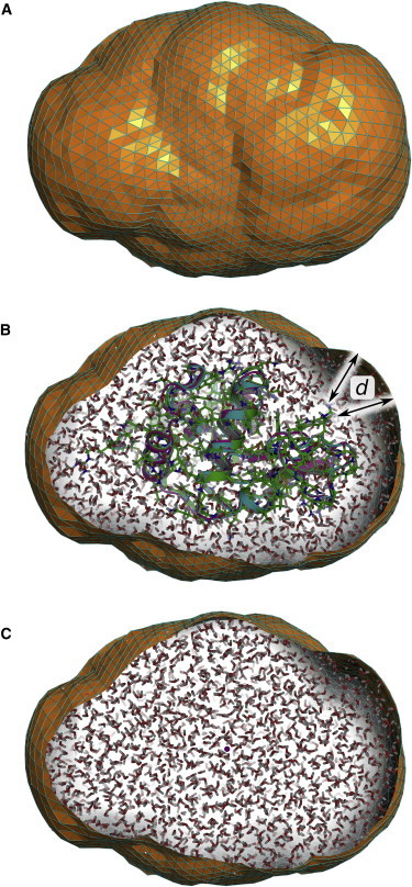
Spatial envelope around lysozyme, separating the protein and the solvation layer from bulk water. (A) The envelope at a distance of 6 Å from lysozyme, defined by 5120 triangular faces. (B) Lysozyme with the solvation layer. (C) Excluded solvent defined by the envelope. To see this figure in color, go online.
The envelope allows one to divide the instantaneous electron densities as follows:
| (7) |
| (8) |
where the subscript i and o indicate electron density inside and outside of the envelope, respectively. To evaluate , the following three assumptions are applied (24): 1), The average electron densities outside of the envelope are equal, . 2), Because the average electron density of the pure-solvent system, , is homogeneous, deviates from zero only at macroscopic length scales that are not measured by the scattering experiment, allowing one to use . 3), Density correlations between the inside and the outside of the envelope are only relevant in the vicinity of the envelope surface. Moreover, because the solvent is bulk-like at surface, such correlations are identical in the A and in the B system, allowing one to simplify it as follows:
| (9) |
Using the above-mentioned equations, and evaluating the respective Fourier transforms yields the following:
| (10) |
where the asterisk denotes the complex conjugate. The first and second term in Eq. 10 are the scattering intensities from the atoms inside of the envelope of the A and B systems, respectively. The third term represents the correlation between 1), the bulk water outside of the envelope, and 2), the density contrast between the A and B systems inside the envelope. Because Eq. 10 involves only densities inside of the envelope, it can be computed from an MD simulation of a protein in a finite simulation box. We note that Eq. 10 is equivalent to , which takes the form of Eq. 26 from Park et al. (24). However, in Park et al. (24) the average over the solvent was conducted at frozen protein coordinates, whereas Eq. 10 involves the average over both solvent and solute degrees of freedom.
Computational details
Atomic form factors
Given the coordinates of atoms within the envelope, the scattering amplitude for an individual simulation frame is written as follows:
| (11) |
where is the number of atoms within the envelope, are the atomic form factors, and is the coordinate of atom j. The analogous relation is applied to compute . The form factors are well approximated as follows:
| (12) |
where , , c are the Cromer-Mann parameters (29), which are published in the tables in (30). To account for electron-withdrawing effects in water molecules, we applied the correction proposed by Sorenson et al. (31) to the form factors, , with the parameters , , and .
Spherical average
The spherical average was computed numerically. For each absolute value of the scattering angle q, a set of vectors was distributed homogeneously on the surface of a sphere with radius q. Here, we generated the vectors using the spiral method, as done previously (24). For simplicity, we used a constant value of in this study, unless otherwise noted. As we will discuss, the best computational efficiency is achieved if J is chosen as a function of q.
Construction and use of the envelope
Various polygon mesh approaches can be employed to represent the envelope surface. In this work, we constructed the envelope from an icosphere, which was built from a regular icosahedron by recursively subdividing its triangular faces into four triangles. Upon each recursion, new vertices were projected in radial direction onto the unit sphere. After M recursions, an icosphere with triangular faces is obtained. For the present purpose, we found M = 4 to be sufficient. Subsequently, the icosphere is centered at the center of mass of the solute, and the vertices of the envelopes are moved in radial direction until each vertex has a distance of at least d from all solute atoms. If the envelope is constructed from multiple simulation frames, the solute is first superimposed onto a reference structure by a mean-square-fit. The envelope around lysozyme at a distance d = 0.6 nm from the protein is shown in Fig. 1 A.
Given the envelope, the solvation layer is constructed from a simulation frame using the protocol described in the Supporting Material. The protocol ensures that no pairs of solvent atoms corresponding to periodic images are inside of the envelope, which would generate spurious periodicity. Simultaneously, however, the protocol avoid tests over all neighboring periodic images of solvent atoms, hence allowing a computationally efficient construction of the solvation layer.
Solvent density correction
The excess intensity I(q) at small scattering angles is very sensitive to the density of the applied water model. However, some popular water models such as TIP3P (32) or SPC (33) reproduce the experimental water density only approximately. In addition, some water models were originally parameterized for the use with Coulomb cutoffs, whereas Ewald summation methods have become the de facto standard in MD simulations. Consequently, the water density may be affected (34,35). Moreover, because of finite-size effects, water density and correlations may slightly differ between the pure-solvent simulation and a protein simulation, which may prevent I(q) from converging with increasing thickness d. Therefore, Köfinger and Hummer scaled the solvent density and radial distribution functions to match the solvent properties between solute and pure-solvent simulations (25). In a related approach, Oroguchi and Ikeguchi modified the solvent density to account for different ion concentrations (36).
In this study, we applied a density correction to the solvent of the A and B systems, respectively, where and denote the experimental density and the bulk density (outside of the envelope). For the B system, this corresponds to a correction of the amplitude by . Here, denotes the Fourier transform and is an indicator function that takes unity inside and zero outside of the envelope. In the A system, the density correction was only applied to the solvation shell, that is, , where denotes the solvent density in the envelope. The Fourier transform was numerically evaluated using volume bins, where is the number of faces of the envelope (5120 in this study). The effect of the correction is presented in the Results section.
Computational cost and convergence
Most of the computational effort is spent for the calculation of the scattering amplitudes and (Eq. 11), requiring sine and cosine evaluations for each simulation frame. Here, and are the number of scattering atoms within the envelope of the solute and pure-solvent system, respectively; and is the number of absolute q values. The parameter determines the number of -vectors for each absolute scattering vector to take the spherical average (see previous explanation). Following Gumerov et al. (37), that parameter should be taken as , where D is the maximum diameter of the envelope, and α is a constant that determines the accuracy of the numerical average. As shown in Fig. S8 A, we determined a possible choice for α by evaluating the convergence of the WAXS curves with increasing and found that yields the spherical average within an accuracy of 2%. To estimate the minimum required computational cost to compute the information contained a WAXS curve, let according to the number of Shannon channels (1,38), which yields . Here, we approximated . For spherical solutes, the required number of sin/cos evaluations can be rewritten as , where we simplified , and where is the particle number density (approximately 100 nm-3 for biomolecular systems). Hence, the cost per frame scales quadratically with the particle number in the envelope, yet with a very small prefactor.
The number of simulation frames that is required to compute a converged WAXS curve was estimated using solutes that cover a wide range of sizes: GB3, ubiquitin, lysozyme, glucose isomerase, and the ribosome (Fig. S8, B and C). The analysis suggests that rapidly decays with the particle number N. Therefore, the cost for the calculation of a converged WAXS curve scales significantly better than .
As a numerical example, the average over 1000 frames of a lysozyme simulation requires sin/cos evaluations (, , constant ). That calculation required 12 min on an 16-core server node with Intel Xeon E5-2670 (2.6GHz; Santa Clara, CA) processors, which was possible by employing efficient single instruction/multiple data (SIMD) instructions such as streaming SIMD extensions or advanced vector extensions for simultaneous sine/cosine evaluations, as implemented in GROMACS (39). We note, however, that reasonable convergence can be achieved by an average over 100 simulation frames, thus allowing intensity calculations on a modern desktop computer in several minutes. The calculations presented here were implemented into a modified version of the GROMACS simulation software, version 4.62 (39).
Molecular dynamics simulations
The initial structures for lysozyme, ubiquitin, GB3, cytochrome C, and glucose isomerase were taken from the Protein Data Bank (PDB; codes 193L, 1D3Z, 1IGD, 1CRC, and 1MNZ, respectively (40–43)). The four N-terminal residues of GB were removed, as was done in the previous experiments (20,25). Organic molecules from the crystallization buffer (if present) were removed. Crystal water as well as Ca2+ and Mg2+ ions (if present) were kept in the structure. Hydrogen atoms were added with the pdb2gmx software (39), with the exception of His-220 of GI, which was protonated at the atom. The structures were placed into a simulation box of a dodecahedron, keeping a distance of at least 1.3 nm to the box boundary. The simulation boxes were filled by explicit water molecules of the respective model applied, and the systems were neutralized by adding the required number of Na+ or Cl− atoms. The energy of the systems was minimized with a steepest-descent algorithm. Before production simulation, each system was equilibrated for 50 ps with position restraints applied to the backbone or to all heavy atoms (force constant ). The simulation system of the ribosome was taken from a previous study (44).
All simulations were carried out using the Gromacs simulation software, version 4.6 (39). To test the influence of the applied force field parameters, we conducted simulations using various protein force field/water model combination. Accordingly, the proteins were described by the CHARMM22∗ (45,46), CHARMM27 (47), Amber99SB (48), Amber03 (49), or by the OPLS all-atom force field (50). The following water models were tested for this study: TIP3P (32), CHARMM-TIP3P (TIPSP3) (45), TIP4P (32), TIP4P-Ew (51), TIP5P (34), TIP5P-Ew (35), SPC (33), and SPC/E (52). The temperature was controlled at 300 K through velocity rescaling (53) , and the pressure was kept at 1 bar using the weak coupling scheme (54) . The SETTLE (55) algorithm was applied to constrain bond lengths and angles of water molecules, and LINCS (56) was used to constrain all other bond lengths, allowing a time step of 2 fs. Electrostatic interactions were calculated using the particle-mesh Ewald method (57,58), and dispersive interactions were described by a Lennard-Jones potential with a cutoff at 1 nm. The pressure was corrected for the missing dispersion interactions beyond the cutoff.
The density profiles (Fig. 3 B) were computed using a series of calculations with increasing distance d of the envelope from the solute. The density was subsequently computed from the differences between those calculations in the average number of electrons inside the envelope.
Figure 3.
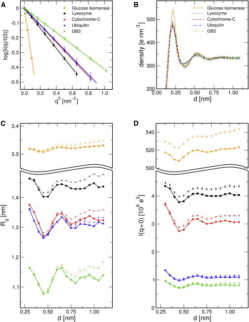
Analysis of the solvation layer. (A) Typical Guinier fits (lines) to the calculated intensities (symbols), , allowing one to extract the radius of gyration and I(q = 0). (B) Density of the solvent versus distance d from the protein atomic centers. (C) Radii of gyration and (D) I(q = 0), as extracted form the Guinier fits, are plotted versus the thickness of the solvation layer d. Colors and symbols are chosen as indicated in the legend of A. Solid curves: with solvent density correction; dotted curves: without solvent density correction. To see this figure in color, go online.
Results and Discussion
Calculated versus experimental profiles
Fig. 2 A presents WAXS profiles from simulations of glucose isomerase, hen egg-white lysozyme, cytochrome C, ubiquitin, and of the B3 domain of protein G (GB3). Molecular representations of the proteins are shown in Fig. 2, B–F. The profiles were computed from an average over 1000 frames taken from 10-ns simulations with position restraint potentials on the backbone atoms , using the CHARMM22∗ and the TIP3P water model. The envelope was constructed at a distance of from the protein atoms. The role of d is analyzed below in more detail.
Figure 2.
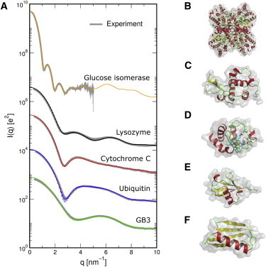
Comparison between calculated and experimental SAXS/WAXS patterns. (A) Colored curves (thin black in print version): simulated patterns of five different proteins, as indicated in the graph; gray curves: experimental patterns fitted to the simulation result using a single fitting parameter. Excellent agreement is found. For clarity, the intensities for the five proteins were scaled by (from top to bottom) constants of 10, 1, 0.1, 0.01, and 0.001, respectively. Experimental profiles were taken from earlier studies (20,59). (B–F) Molecular images of glucose isomerase, lysozyme, cytochrome C, ubiquitin, and GB3, respectively. To see this figure in color, go online.
To validate the calculations, we fitted experimental profiles to the calculated profiles by minimizing as follows:
| (13) |
where denotes the number of q points (typically 100), and are the calculated and the experimental intensities, respectively, and log is the natural logarithm. Here, we decided to fit the experimental rather than the calculated profiles, because the latter do not contain any free parameters. In addition, we carried out a nonweighted fit on a logarithmic intensity scale to equally account for both the small and the wide-angle regimes. Hence, besides the overall scaling parameter f, only a single parameter c was fitted, which aims to account for experimental uncertainties from the buffer subtraction and, optionally, from residual dark currents. Experimental SAXS/WAXS profiles were taken from earlier studies (20,59). The fitted experimental profiles are shown in gray in Fig. 2 A, demonstrating excellent agreement both at small and at wide angles.
Previous studies typically used the experimental statistical errors as inverse fitting weights, putting very strong weights to small angles. To facilitate the comparison with previous studies, Fig. S1 presents results from a weighted fitting procedure, again demonstrating very good agreement over the entire q-range. To illustrate the effect of the fitting parameter c (Eq. 13), we further restricted the fit to the range using only the overall scale f, while setting the parameter c to zero (Fig. S2). Here, experimental curves are systematically above the calculated curves at high angles, suggesting that, indeed, either a systematic error in the buffer subtraction or residual dark currents may have contributed to deviations between simulation and experiment.
Analysis of the solvation layer
The distance of the envelope d from the solute atoms must be sufficiently large to ensure bulk-like water at the envelope surface. If d is chosen too small, density modulations due to the first and second solvation layer may systematically bias the calculated profiles. On the other hand, an unnecessarily large d adds noise to the profiles, because the intensities of the solute system (including its solvation layer) and of the excluded solvent rapidly increase with d, whereas the excess intensity should converge with increasing d.
Here, simulations were carried out using TIP4P-Ew water and applying position restraints on all heavy atoms to minimize contributions from protein fluctuations. To find the optimal choice for d, we extracted the radius of gyration and the intensity at zero angle from the Guinier fit, , which is valid up to for globular proteins (1). Typical Guinier fits are shown in Fig. 3 A. Fig. 3, C and D presents and versus d, visualizing the effects of the first and second solvation layer on the SAXS profiles. The influence of d on the intensity at wide angles is shown in Fig. S3.
As expected, the effects of the solvation layer on and are more prononced for small proteins such as GB3, ubiquitin, and cytochrome C (Fig. 3, green, blue, red). This demonstrates the importance of accurately modeling the density of the solvation layer for these cases. For instance, a distance of only 3 Å includes the first solvation layer, but it would miss the reduced density just behind the first solvation layer, thereby overestimating (compare Fig. 3 B). In contrast, would lead to an underestimate of , because it misses the increased density because of the second solvation layer at .
In principle, and should converge with increasingly bulk-like solvent behind the second solvation shell. However, we observed a systematic drift both in and at (Fig. 3, B and C, dotted lines), which we traced to a slightly different bulk water density in the protein and pure-solvent simulations. Therefore, we applied a density correction that allows us to fix the bulk water density to the experimental value of . (See Materials and Methods for details.) This correction removed the drift almost completely (Fig. 3, B and C, solid lines). The very weak drift in the curves for glucose isomerase (Fig. 3, B and C, orange), we believe, originates from the large counter ion cloud of 60 sodium ions present in those simulations. Notably, altering the solvent density with the aim to model the complex buffer did not systematically improve the agreement between calculated and experimental WAXS curves. Based on the curves in Figs. 3, B and C and S3, we constructed the envelope using throughout this study, close to the value of 7 Å suggested by Park et al. (24).
Role of the water model
A variety of different explicit water models were developed during the past decades, which differ significantly in terms of their density and structure factors. Hence, the water model may influence the calculated SAXS/WAXS profiles via three effects. 1), The excess intensity scales at small scattering angles q with the square of the density contrast between solute and water, and it is therefore very sensitive to the density of the applied water model. However, as shown below, our procedure to fix the bulk density at the experiential value corrects for those effects (see also previous paragraph and Materials and Methods). 2), The packing of different water models on the protein surface may differ, thereby changing the structure of the solvation layer. 3), Variations of the water structure factor (31) may be relevant at wide angles, where the water scattering becomes dominant.
WAXS profiles were computed using eight different popular water models, and they are analyzed in detail in Fig. 4. The simulations were conducted with position restraints on all heavy atoms to ensure that differences between WAXS patterns originate exclusively from the applied water model. The overall shape of the SAXS and near-WAXS profiles are indistinguishable between different water models (Fig. 4 A). The same is true also when different all-atom force fields for the protein are applied (Fig. S4). In contrast, without solvent density correction, may vary by up to 30% (Fig. S5). We note that those large variations of originate from variations in the density contrast, and not by a possible mismatch in the bulk water densities of solute and solvent simulation systems. Because the water density mainly affects at small angles, those variations cannot be absorbed by the fitting parameters c or f (Eq. 13). In the far wide-angle regime around the water peak, however, significant differences appear that reflect variations in the structure of the water models (Fig. 4 B, lower curves). These differences are to be expected, because popular water models such as TIP3P (32) or SPC (33) were found to lack structure of the second solvation shell (31), whereas the structure of SPC/E and of the TIP4P and TIP5P variants are in better agreement with x-ray scattering data (31,51).
Figure 4.
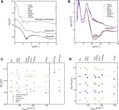
Role of the water model for SAXS/WAXS patterns. (A) SAXS and near-WAXS curves for three proteins (as indicated in the graph) computed using eight different water models, as shown in the legend. The curves from different water models are indistinguishable. (B) Far-WAXS patterns of ubiquitin. Significant differences appear around the water peak between 15 and 35 nm-1. Lower and upper curves: buffer subtraction schemes and , respectively. (C) Difference between the radius of gyration computed from the Guinier fit and computed from the crystal or NMR structure, demonstrating the increased because of higher water density in the solvation layer. is plotted versus the electron density of the water model. Systematic differences because of 1), the protein and 2), the water model are visible. Right-hand side: results from CRYSOL (default parameters), and experimental estimates. The color/symbol coding is indicated in the legend. (D) Intensity at q = 0, with the same color/symbol coding as in C. For clarity, I(q = 0) was multiplied by a different constant for each protein. Dotted lines in C and D are the average values for the respective protein shown to guide the eye. To see this figure in color, go online.
In addition, Fig. 4 B illustrates the influence of the buffer subtraction scheme. The lower curves where computed following Eq. 1, where the negative intensities reflect that the scattering intensity of the excluded solvent is larger around nm−1 than the scattering of the protein. The upper curves in Fig. 4 B correspond to the subtraction scheme involving the volume fraction of the protein, , and they were computed following an earlier study (25). For that scheme, pure water scattering is added back, leading to reduced influence of the water model.
To analyze the impact of the water model on the solvation layer, Fig. 4, C and D, presents and extracted from the Guinier fit, plotted versus the density of the respective water model (as indicated on top of the graphs). Here, we plotted the difference to the value taken from the crystal or NMR structure, thus visualizing purely the increase in because of the solvation layer. Remarkably, highly differs between different proteins. The influence of the water model is, however, relatively small, with the exception that TIP5P and TIP5P-Ew overestimate for the four smaller proteins. That finding is in line with a recent simulation study that reported tighter packing of TIP5P around a peptide described by different AMBER force fields, as compared with the default TIP3P water (60). The right-hand side panel of Fig. 4 C shows the estimate for from the experimental SAXS curves, as well as computed by CRYSOL (15) using the default parameters. We find reasonable agreement between simulation and experiment, whereas the implicit solvent model of CRYSOL, as expected, cannot account for variations in the solvation layer without fitting to experimental data.
To summarize, there is no optimal water model for the entire q range. Up to scattering angles of , we thus recommend the default water model of the applied protein force field. In the far wide-angle regime SPC/E, TIP4P, or TIP4P-Ew are more appropriate to reproduce the water scattering peak. If the protein atoms are not restrained, however, a validation is required to exclude the possibility that the water model leads to unphysical population of conformational states. It is important to note that our conclusions here are drawn using CHARMM22∗ (46), and may not necessarily apply to other force fields. We do not recommend TIP5P variants for CHARMM22∗ because they may overestimate .
Importance of atomic fluctuations
Most established methods for the calculation of SAXS/WAXS profiles use static biomolecular structures (15–18,20,24). However, WAXS profiles detect short-range correlations that may be smeared out by thermal fluctuations, thereby changing the scattering profiles. Indeed, Tiede et al. reported that incorporating B-factors improves the agreement between calculated and measured profiles in the regime, suggesting that atomic fluctuations are relevant here (61). Therefore, to quantify the influence of atomic fluctuations on WAXS profiles we conducted a series of simulations over a range of protein flexibilities: 1), all protein atoms were constrained (frozen); 2), all heavy atoms were restrained (force constant ); and 3), only backbone atoms were restrained ; or 4), free (unrestrained) simulations. For each setup, the WAXS spectrum was computed from ∼ 5000 simulations frames, and the deviation χ to the experimental data was computed by minimizing Eq. 13. In addition, to test how the fitting metric influences the agreement between computed and experimental curves, the fits were also conducted using the experimental statistical errors as inverse weights (Table S1).
As shown in Table 1, the agreement between the calculated and the experimental WAXS curves improves as we incorporate atomic fluctuations up to backbone-restraints. Results from the weighted fits corroborate this finding. However, compared with the nonweighted fits on the logarithmic scale, a smaller influence from fluctuations is found. This suggest that fluctuations are indeed particularly relevant for the wide-angle regime, which is emphasized by a nonweighted fit. A notable exception is the agreement for GB3 that is strongly dependent on the fitting procedure, which, we believe, indicates that systematic errors in buffer subtraction dominate the analysis.
Table 1.
Effect of atomic fluctuations and conformational sampling on WAXS profiles
| Frozena | Posres heavy atb | Posres backbonec | Free MD 1 | Free MD 2 | NMR ensemble | |
|---|---|---|---|---|---|---|
| Glucose isomerase | 5.8 | 5.4 | 5.4 | 12.1 (100 ns) | ||
| Lysozyme | 9.0 | 7.2 | 7.2 | 8.0 (1 ) | 10.9 (1 ) | 11.9e |
| Cytochrome C | 9.8 | 8.9 | 4.7 | 3.9 (20 ns) | ||
| Ubiquitin | 14.1 | 9.4 | 7.8 1.2d | 5.8 (1 ) | 6.3 (1 ) | 6.9f / 7.0g |
| GB3 | 9.6 | 9.7 | 6.5 0.7d | 8.3 (1 ) | 7.5 (1 ) |
from simulations with decreasing restraints on the protein.
All protein coordinates frozen.
Position restraints on all heavy atoms .
Position restraints on backbone atoms only .
Average and standard deviation from 10 independent simulations.
The respective WAXS profiles for cytochrome C and ubiquitin are shown in Fig. 5 A. The WAXS profiles of ubiquitin are nearly unaffected by fluctuations at small angles, but they highly differ at wide angles (compare black and red curves). In contrast, the profiles of cytochrome C differ only moderately at wide angles. Instead, the intensity at small angles decreases and the peaks around are left-shifted, indicating that cytochrome C expands upon the relaxation of the restraints. Hence, the improved agreement between experimental and computed WAXS patterns for cytochrome C may be taken as an indication that its crystal structure is more compact than the solution structure.
Figure 5.
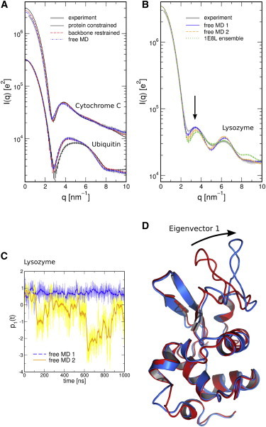
Role of side-chain and loop fluctuations in WAXS profiles. (A) WAXS profiles for cytochrome C and ubiquitin computed from simulations with increasing flexibility, as indicated in the legend. Thick gray: experimental curve fitted to the curve from the free MD simulation, using only a single fitting parameter. (B) WAXS profiles for lysozyme computed from two 1 μs simulations or from the 1E8L NMR ensemble. The arrow indicates the region with the largest discrepancy between the two simulations. (C) Projection on the first PCA eigenvector of the two free MD simulations. (D) Visualization of the first PCA vector. To see this figure in color, go online.
Validating solution ensembles against WAXS data
We conducted free MD simulations between 20 ns and 1 μs to 1), quantify the role of conformational sampling on WAXS profiles, and 2), to investigate the sensitivity of χ with respect to potential unphysical biases in a solution ensembles. Compared with simulations with restraints on the backbone, the agreement to experiment systematically improved for ubiquitin, but it slightly degraded or depended on the weights for GB3 and cytochrome C, respectively (Tables 1 and S1). These findings suggest that 1), conformational sampling of the backbone does not significantly improve WAXS curves for the relatively stable proteins studied here; and that 2), the MD simulations generate reasonably correct ensembles of those proteins in solution.
We noted that free simulations resulted in a significant increase of χ for glucose isomerase ( versus ), as well as during the second microsecond-simulation of lysozyme ( versus ). A closer inspection of the glucose isomerase simulation showed that the drastic increase of χ is linked to an increase of by 1 Å during the first 20 ps of the simulations. Hence, the experimental SAXS curve suggests that the increase of during the simulation was unphysical. We repeated the simulations in four variations: 1) using different protein force fields (Amber99SB (48), or OPLS-aa (50)), 2) using longer 10 ns-equilibration with position restraints, 3) using gradual instead of instantaneous relaxation of position restraints after equilibration, or 4) simulating with 150 mM sodium chloride instead of using only counter ions. However, the increase of and, hence, of χ was consistently reproduced. In this study, we do not aim to clarify whether the instability might be attributable to bad conformations in the 1MNZ structure, or attributable to incomplete electrostatic screening around the highly charged protein. Instead, the analysis demonstrates that the comparison with experimental SAXS data is a highly sensitive measure to either validate simulation ensembles or to detect nonphysical conformations.
The increased χ during the second MD simulation of lysozyme can by explained by means of a principal component analysis on the backbone atoms, which was conducted after merging the two independent simulations (Fig. 5, B–D). The first principal component (PC) is presented in Fig. 5 C, showing that the second simulation fluctuated along the first PC, whereas the first simulation remained stable. The first PCA vector is visualized in Fig. 5 D and mainly corresponds to enhanced flexibility of the loop between residue numbers 60 and 80. Using CRYSOL calculations from the full protein and from structures lacking that loop, we confirmed that this loop motion accounts for differences between the WAXS curves of the two simulations (Fig. S6). Hence, the increased χ from the second lysozyme simulation suggests that this loop is instead stable in solution. More importantly, the results further confirm that WAXS calculations are sufficiently sensitive to detect the flexibility of a single loop, thereby opening the route to apply WAXS profiles for the validation of force field-based simulations.
To further investigate the role of conformational sampling for WAXS profiles, we computed the profiles from two different NMR ensembles of ubiquitin (PDB codes 1XQQ (62) and 1D3Z (41)) and one NMR ensemble of lysozyme (PDB code 1E8L (63), Fig. 5 B, green). Each conformer of the ensemble was simulated for 2 ns with position restraints on the backbone atoms (). Subsequently, the WAXS profiles were computed from ∼5000 frames that were uniformly taken from the individual conformer simulations. The agreement to experiment as quantified by χ-values is shown in Table 1. The profiles of the two ubiquitin ensembles 1XQQ and 1D3Z favorably agree with experiment (6.9 and 7.0 ), but they do not outperform the microsecond MD simulations, suggesting that the simulations correctly represent the solution state of ubiquitin. The spectrum of the 1E8L ensemble of lysozyme, however, only moderately agrees with the experiment, suggesting that the 193L crystal structure better represents the solution state of lysozyme.
Taken together, we find that incorporating atomic fluctuations by means of position restraints on the backbone atoms significantly improves the agreement between theoretical and experimental WAXS profiles. Including additional conformational sampling by free MD simulations leads to more accurate predictions only in certain cases, such as for ubiquitin. Therefore, position-restrained simulations are suitable for reliable predictions of WAXS profiles. It is important to note, however, that we here studied relatively stable proteins. For flexible peptides or protein domains connected by flexible linkers, conformational sampling is crucial to predict SAXS/WAXS patterns (6,27,28). In turn, we find that calculated WAXS profiles are highly sensitive with respect to minor conformational transitions of the protein, such as the flexibility of a single loop or alterations of the radius of gyration. Therefore, the quantitative comparison between MD simulations and WAXS patterns shown here emerges as a tool to test the accuracy of solution ensembles.
Conclusions
The information content of SAXS/WAXS curves is relatively low; most measured curves contain only 10 to 15 independent data points (1). Free parameters that are fitted to match calculated and experimental profiles further reduce the information that is effectively available for grounding structural interpretations. Free parameters also increase the risk of drawing unfounded conclusions because of overfitting. Apart from the overall scaling factor for scattering intensities, we used only a single additional fitting parameter that accounts for experimental uncertainties attributable to the buffer subtraction and to dark currents, thereby minimizing the risk of overfitting, similar to a recent MD study (25). In particular, no free parameters are required to model the scattering contributions from the solvation layer and from the excluded solvent. In that respect, our calculations contrast methods based on implicit solvation models and/or on atomic form factors that are reduced according to the displaced solvent (13,15–18,22). It is important to note that the distance d between protein and envelope is not a free parameter in our calculations. Instead, was chosen sufficiently large to ensure bulk-like water at the surface of the envelope. Likewise, we do not consider the force field as free parameters, because they are typically based on ab initio calculations and previously refined with respect to independent experimental data, such as solvation free energies or NMR data. Here, neither d nor the force field parameters are fitted to match the calculated and experimental WAXS profiles.
The algorithms shown in this study are efficient and can be parallelized, allowing one to compute WAXS patterns even from simulations of large macromolecular assemblies. To illustrate this fact, we computed the WAXS spectrum from an MD simulation of the E. coli ribosome (Fig. 6) (44). The envelope contained ∼820,000. By averaging over 20 simulations frames we achieved nearly invisible small error bars, and the calculation took 1.25h on a 64-core AMD Opteron server (Sunnyvale, CA). Hence, the computational cost of the WAXS calculations presented in this study are negligible compared with the cost of the respective MD simulation. To reduce the cost of the WAXS calculations, we modeled the solvation layer by an irregular envelope instead of a sphere (25), which significantly reduces the number of water molecules that must be included in the calculations, thereby also reducing statistical noise in the density contrast to the pure-solvent system. For instance, an envelope and a sphere around ubiquitin, each at a distance of 8 Å from the protein atoms, contain ∼1550 and ∼3700 water molecules, respectively. This increase will be more drastic for more elongated solutes.
Figure 6.
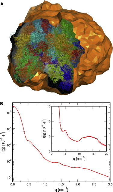
SAXS/WAXS patterns of the E. coli Ribosome. (A) Atomistic simulation system of the ribosome. Ribosome atoms are represented as sticks, and water is not shown for clarity. The envelope (clipped surface) at a distance of 8 Å from the ribosome. (B) SAXS pattern and (inset) WAXS pattern of the ribosome, averaged from 20 simulation frames and using J = 8000. Error bars (hardly visible) indicate one SD. To see this figure in color, go online.
The calculated WAXS profiles are in excellent agreement to experimental data both in the small and in the wide-angle regime. To establish WAXS calculations from MD simulations as a robust and predictive tool, we carefully evaluated the role of the applied force fields on the profiles. We found that both the protein and the water force field have only a minor effect on the profiles up to 15 nm−1, once we corrected for inaccurate densities of certain water models (Figs. 4 and S4). Hence, popular water models such as TIP3 or SPC are suitable for WAXS calculations up to 15 nm−1, despite the fact that these models lack structure in the second solvation shell (31). In contrast, the intensities are significantly affected by the water model at very high angles, where the water scattering becomes dominant. At such angles, however, additional factors may complicate the calculations of WAXS profiles such as inelastic scattering or electron-withdrawing effects along polarized bonds. It will therefore be highly interesting to test our calculation against experimental profiles also in the far wide-angle regime in a future study.
We used the methodology to investigate the role of side chain fluctuations and conformational sampling in solution scattering. We found that including fluctuations by means of position-restraint simulations yield better agreement with experimental SAXS/WAXS profiles, demonstrating the importance of atomic fluctuations for wide-angle scattering.
Solution ensembles generated from free MD simulations up to one microsecond provide only in certain cases a more accurate solution state of the protein, as quantified from the deviation χ between calculated and experimental WAXS profiles. We found that small conformational transitions, such as an unphysical increase of glucose isomerase by 1% (or 0.3 Å) or an increased flexibility of a single loop of lysozyme, may lead to a significant discrepancy between simulation and experiment. In turn, consistently small χ-values, as observed for microsecond simulations of ubiquitin, suggest that the simulations correctly sample the solution state of that protein. Hence, comparing MD simulations with experimental WAXS profiles emerges as a new route to validate solution ensembles, complementary to established protocols based on NMR or circular dichroism data (64–66).
To make the algorithms used here available to the public, we are currently setting up a web server for automated MD simulations and WAXS calculations. We expect the web server to go online in the coming months at: http://waxsis.uni-goettingen.de.
Acknowledgments
We are grateful to Lachlan Casey for the experimental SAXS curve of glucose isomerase, and to Alexander Grishaev for the experimental WAXS curves of lysozyme, cytochrome C, ubiquitin, and GB3. We thank Lars Bock and Helmut Grubmüller for the simulation system of the ribosome, and we thank Kalina Atkovska fore carefully reading the manuscript.
This study was supported by the Emmy-Noether program of the Deutsche Forschungsgemeinschaft (HU 1971/1-1).
Supporting Material
Supporting Citations
Reference (67) appears in the Supporting Material.
References
- 1.Putnam C.D., Hammel M., Tainer J.A. X-ray solution scattering (SAXS) combined with crystallography and computation: defining accurate macromolecular structures, conformations and assemblies in solution. Q. Rev. Biophys. 2007;40:191–285. doi: 10.1017/S0033583507004635. [DOI] [PubMed] [Google Scholar]
- 2.Koch M.H., Vachette P., Svergun D.I. Small-angle scattering: a view on the properties, structures and structural changes of biological macromolecules in solution. Q. Rev. Biophys. 2003;36:147–227. doi: 10.1017/s0033583503003871. [DOI] [PubMed] [Google Scholar]
- 3.Graewert M.A., Svergun D.I. Impact and progress in small and wide angle x-ray scattering (SAXS and WAXS) Curr. Opin. Struct. Biol. 2013;23:748–754. doi: 10.1016/j.sbi.2013.06.007. [DOI] [PubMed] [Google Scholar]
- 4.Makowski L., Rodi D.J., Fischetti R.F. Characterization of protein fold by wide-angle x-ray solution scattering. J. Mol. Biol. 2008;383:731–744. doi: 10.1016/j.jmb.2008.08.038. [DOI] [PubMed] [Google Scholar]
- 5.Fischetti R.F., Rodi D.J., Makowski L. Wide-angle x-ray solution scattering as a probe of ligand-induced conformational changes in proteins. Chem. Biol. 2004;11:1431–1443. doi: 10.1016/j.chembiol.2004.08.013. [DOI] [PubMed] [Google Scholar]
- 6.Zagrovic B., Pande V.S. Simulated unfolded-state ensemble and the experimental NMR structures of villin headpiece yield similar wide-angle solution x-ray scattering profiles. J. Am. Chem. Soc. 2006;128:11742–11743. doi: 10.1021/ja0640694. [DOI] [PubMed] [Google Scholar]
- 7.Makowski L., Bardhan J., Fischetti R.F. WAXS studies of the structural diversity of hemoglobin in solution. J. Mol. Biol. 2011;408:909–921. doi: 10.1016/j.jmb.2011.02.062. [DOI] [PMC free article] [PubMed] [Google Scholar]
- 8.Cammarata M., Levantino M., Ihee H. Tracking the structural dynamics of proteins in solution using time-resolved wide-angle x-ray scattering. Nat. Methods. 2008;5:881–886. doi: 10.1038/nmeth.1255. [DOI] [PMC free article] [PubMed] [Google Scholar]
- 9.Andersson M., Malmerberg E., Neutze R. Structural dynamics of light-driven proton pumps. Structure. 2009;17:1265–1275. doi: 10.1016/j.str.2009.07.007. [DOI] [PubMed] [Google Scholar]
- 10.Ahn S., Kim K.H., Ihee H. Protein tertiary structural changes visualized by time-resolved x-ray solution scattering. J. Phys. Chem. B. 2009;113:13131–13133. doi: 10.1021/jp906983v. [DOI] [PubMed] [Google Scholar]
- 11.Malmerberg E., Omran Z., Neutze R. Time-resolved WAXS reveals accelerated conformational changes in iodoretinal-substituted proteorhodopsin. Biophys. J. 2011;101:1345–1353. doi: 10.1016/j.bpj.2011.07.050. [DOI] [PMC free article] [PubMed] [Google Scholar]
- 12.Kim K.H., Oang K.Y., Ihee H. Direct observation of myoglobin structural dynamics from 100 picoseconds to 1 microsecond with picosecond x-ray solution scattering. Chem. Commun. (Camb.) 2011;47:289–291. doi: 10.1039/c0cc01817a. [DOI] [PMC free article] [PubMed] [Google Scholar]
- 13.Merzel F., Smith J.C. Is the first hydration shell of lysozyme of higher density than bulk water? Proc. Natl. Acad. Sci. USA. 2002;99:5378–5383. doi: 10.1073/pnas.082335099. [DOI] [PMC free article] [PubMed] [Google Scholar]
- 14.Perkins S.J. X-ray and neutron scattering analyses of hydration shells: a molecular interpretation based on sequence predictions and modelling fits. Biophys. Chem. 2001;93:129–139. doi: 10.1016/s0301-4622(01)00216-2. [DOI] [PubMed] [Google Scholar]
- 15.Svergun D., Barberato C., Koch M.H.J. CRYSOL—a program to evaluate x-ray solution scattering of biological macromolecules from atomic coordinates. J. Appl. Cryst. 1995;28:768–773. [Google Scholar]
- 16.Liu H., Morris R.J., Zwart P.H. Computation of small-angle scattering profiles with three-dimensional Zernike polynomials. Acta Crystallogr. A. 2012;68:278–285. doi: 10.1107/S010876731104788X. [DOI] [PubMed] [Google Scholar]
- 17.Schneidman-Duhovny D., Hammel M., Sali A. Accurate SAXS profile computation and its assessment by contrast variation experiments. Biophys. J. 2013;105:962–974. doi: 10.1016/j.bpj.2013.07.020. [DOI] [PMC free article] [PubMed] [Google Scholar]
- 18.Azuara C., Orland H., Delarue M. Incorporating dipolar solvents with variable density in Poisson-Boltzmann electrostatics. Biophys. J. 2008;95:5587–5605. doi: 10.1529/biophysj.108.131649. [DOI] [PMC free article] [PubMed] [Google Scholar]
- 19.Fraser R.D.B., MacRae T.P., Suzuki E. An improved method for calculating the contribution of solvent to the x-ray diffraction pattern of biological molecules. J. Appl. Cryst. 1978;11:693–694. [Google Scholar]
- 20.Grishaev A., Guo L., Bax A. Improved fitting of solution x-ray scattering data to macromolecular structures and structural ensembles by explicit water modeling. J. Am. Chem. Soc. 2010;132:15484–15486. doi: 10.1021/ja106173n. [DOI] [PMC free article] [PubMed] [Google Scholar]
- 21.Bardhan J., Park S., Makowski L. SoftWAXS: a computational tool for modeling wide-angle x-ray solution scattering from biomolecules. J. Appl. Cryst. 2009;42:932–943. doi: 10.1107/S0021889809032919. [DOI] [PMC free article] [PubMed] [Google Scholar]
- 22.Merzel F., Smith J.C. SASSIM: a method for calculating small-angle x-ray and neutron scattering and the associated molecular envelope from explicit-atom models of solvated proteins. Acta Crystallogr. D Biol. Crystallogr. 2002;58:242–249. doi: 10.1107/s0907444901019576. [DOI] [PubMed] [Google Scholar]
- 23.Oroguchi T., Hashimoto H., Ikeguchi M. Intrinsic dynamics of restriction endonuclease EcoO109I studied by molecular dynamics simulations and x-ray scattering data analysis. Biophys. J. 2009;96:2808–2822. doi: 10.1016/j.bpj.2008.12.3914. [DOI] [PMC free article] [PubMed] [Google Scholar]
- 24.Park S., Bardhan J.P., Makowski L. Simulated x-ray scattering of protein solutions using explicit-solvent models. J. Chem. Phys. 2009;130:134114. doi: 10.1063/1.3099611. [DOI] [PMC free article] [PubMed] [Google Scholar]
- 25.Köfinger J., Hummer G. Atomic-resolution structural information from scattering experiments on macromolecules in solution. Phys. Rev. E Stat. Nonlin. Soft Matter Phys. 2013;87:052712. doi: 10.1103/PhysRevE.87.052712. [DOI] [PubMed] [Google Scholar]
- 26.Yang S., Park S., Roux B. A rapid coarse residue-based computational method for x-ray solution scattering characterization of protein folds and multiple conformational states of large protein complexes. Biophys. J. 2009;96:4449–4463. doi: 10.1016/j.bpj.2009.03.036. [DOI] [PMC free article] [PubMed] [Google Scholar]
- 27.Yang S., Blachowicz L., Roux B. Multidomain assembled states of Hck tyrosine kinase in solution. Proc. Natl. Acad. Sci. USA. 2010;107:15757–15762. doi: 10.1073/pnas.1004569107. [DOI] [PMC free article] [PubMed] [Google Scholar]
- 28.Różycki B., Kim Y.C., Hummer G. SAXS ensemble refinement of ESCRT-III CHMP3 conformational transitions. Structure. 2011;19:109–116. doi: 10.1016/j.str.2010.10.006. [DOI] [PMC free article] [PubMed] [Google Scholar]
- 29.Cromer D.T., Mann J.B. X-ray scattering factors computed from numerical Hartree-Fock wave functions. Acta Crystallogr. 1968;A24:321–324. [Google Scholar]
- 30.Brown P.J., Fox A.G., Willis B.T.M. In: 3rd ed. Prince E., editor. Vol. C. Springer; Berlin, Heidelberg, Germany: 2006. pp. 554–595. (International Tables for Crystallography). [Google Scholar]
- 31.Sorenson J.M., Hura G., Head-Gordon T. What can x-ray scattering tell us about the radial distribution functions of water? J. Chem. Phys. 2000;113:9149–9161. [Google Scholar]
- 32.Jorgensen W.L., Chandrasekhar J., Klein M.L. Comparison of simple potential functions for simulating liquid water. J. Chem. Phys. 1983;79:926–935. [Google Scholar]
- 33.Berendsen H.J.C., Postma J.P.M., Hermans J. Interaction models for water in relation to protein hydration. In: Pullman B., editor. Intermolecular Forces. D. Reidel; Dordrecht, The Netherlands: 1981. pp. 331–342. [Google Scholar]
- 34.Mahoney M.W., Jorgensen W.L. A five-site model for liquid water and the reproduction of the density anomaly by rigid, nonpolarizable potential functions. J. Chem. Phys. 2000;112:8910–8922. [Google Scholar]
- 35.Rick S.W. A reoptimization of the five-site water potential (TIP5P) for use with Ewald sums. J. Chem. Phys. 2004;120:6085–6093. doi: 10.1063/1.1652434. [DOI] [PubMed] [Google Scholar]
- 36.Oroguchi T., Ikeguchi M. Effects of ionic strength on SAXS data for proteins revealed by molecular dynamics simulations. J. Chem. Phys. 2011;134:025102. doi: 10.1063/1.3526488. [DOI] [PubMed] [Google Scholar]
- 37.Gumerov N.A., Berlin K., Duraiswami R. A hierarchical algorithm for fast Debye summation with applications to small angle scattering. J. Comput. Chem. 2012;33:1981–1996. doi: 10.1002/jcc.23025. [DOI] [PMC free article] [PubMed] [Google Scholar]
- 38.Shannon C.E., Moore W. University of Illinois Press; Urbana, IL: 1949. The Mathematical Theory of Communication. [Google Scholar]
- 39.Pronk S., Páll S., Lindahl E. GROMACS 4.5: a high-throughput and highly parallel open source molecular simulation toolkit. Bioinformatics. 2013;29:845–854. doi: 10.1093/bioinformatics/btt055. [DOI] [PMC free article] [PubMed] [Google Scholar]
- 40.Vaney M.C., Maignan S., Ducriux A. High-resolution structure (1.33 A) of a HEW lysozyme tetragonal crystal grown in the APCF apparatus. Data and structural comparison with a crystal grown under microgravity from SpaceHab-01 mission. Acta Crystallogr. D Biol. Crystallogr. 1996;52:505–517. doi: 10.1107/S090744499501674X. [DOI] [PubMed] [Google Scholar]
- 41.Cornilescu G., Marquardt J.L., Bax A. Validation of protein structure from anisotropic carbonyl chemical shifts in a dilute liquid crystalline phase. J. Am. Chem. Soc. 1998;120:6836–6837. [Google Scholar]
- 42.Derrick J.P., Wigley D.B. The third IgG-binding domain from streptococcal protein G. An analysis by x-ray crystallography of the structure alone and in a complex with Fab. J. Mol. Biol. 1994;243:906–918. doi: 10.1006/jmbi.1994.1691. [DOI] [PubMed] [Google Scholar]
- 43.Sanishvili R., Volz K.W., Margoliash E. The low ionic strength crystal structure of horse cytochrome c at 2.1 A resolution and comparison with its high ionic strength counterpart. Structure. 1995;3:707–716. doi: 10.1016/s0969-2126(01)00205-2. [DOI] [PubMed] [Google Scholar]
- 44.Bock L.V., Blau C., Grubmüller H. Energy barriers and driving forces in tRNA translocation through the ribosome. Nat. Struct. Mol. Biol. 2013;20:1390–1396. doi: 10.1038/nsmb.2690. [DOI] [PubMed] [Google Scholar]
- 45.MacKerell A.D., Bashford D., Karplus M. All-atom empirical potential for molecular modeling and dynamics studies of proteins. J. Phys. Chem. B. 1998;102:3586–3616. doi: 10.1021/jp973084f. [DOI] [PubMed] [Google Scholar]
- 46.Piana S., Lindorff-Larsen K., Shaw D.E. How robust are protein folding simulations with respect to force field parameterization? Biophys. J. 2011;100:L47–L49. doi: 10.1016/j.bpj.2011.03.051. [DOI] [PMC free article] [PubMed] [Google Scholar]
- 47.Mackerell A.D., Jr., Feig M., Brooks C.L., 3rd Extending the treatment of backbone energetics in protein force fields: limitations of gas-phase quantum mechanics in reproducing protein conformational distributions in molecular dynamics simulations. J. Comput. Chem. 2004;25:1400–1415. doi: 10.1002/jcc.20065. [DOI] [PubMed] [Google Scholar]
- 48.Hornak V., Abel R., Simmerling C. Comparison of multiple Amber force fields and development of improved protein backbone parameters. Proteins. 2006;65:712–725. doi: 10.1002/prot.21123. [DOI] [PMC free article] [PubMed] [Google Scholar]
- 49.Duan Y., Wu C., Kollman P. A point-charge force field for molecular mechanics simulations of proteins based on condensed-phase quantum mechanical calculations. J. Comput. Chem. 2003;24:1999–2012. doi: 10.1002/jcc.10349. [DOI] [PubMed] [Google Scholar]
- 50.Jorgensen W.L., Maxwell D.S., Tirado-Rives J. Development and testing of the OPLS all-atom force field on conformational energetics and properties of organic liquids. J. Am. Chem. Soc. 1996;118:11225–11236. [Google Scholar]
- 51.Horn H.W., Swope W.C., Head-Gordon T. Development of an improved four-site water model for biomolecular simulations: TIP4P-Ew. J. Chem. Phys. 2004;120:9665–9678. doi: 10.1063/1.1683075. [DOI] [PubMed] [Google Scholar]
- 52.Berendsen H.J.C., Grigera J.R., Stroatsma T.P. The missing term in effective pair potentials. J. Chem. Phys. 1987;91:6269–6271. [Google Scholar]
- 53.Bussi G., Donadio D., Parrinello M. Canonical sampling through velocity rescaling. J. Chem. Phys. 2007;126:014101. doi: 10.1063/1.2408420. [DOI] [PubMed] [Google Scholar]
- 54.Berendsen H.J.C., Postma J.P.M., Haak J.R. Molecular dynamics with coupling to an external bath. J. Chem. Phys. 1984;81:3684–3690. [Google Scholar]
- 55.Miyamoto S., Kollman P.A. Settle: An analytical version of the SHAKE and RATTLE algorithms for rigid water models. J. Comput. Chem. 1992;13:952–962. [Google Scholar]
- 56.Hess B. P-LINCS: A parallel linear constraint solver for molecular simulation. J. Chem. Theory Comput. 2008;4:116–122. doi: 10.1021/ct700200b. [DOI] [PubMed] [Google Scholar]
- 57.Darden T., York D., Pedersen L. Particle mesh Ewald: an N ⋅ log(N) method for Ewald sums in large systems. J. Chem. Phys. 1993;98:10089–10092. [Google Scholar]
- 58.Essmann U., Perera L., Pedersen L.G. A smooth particle mesh Ewald method. J. Chem. Phys. 1995;103:8577–8592. [Google Scholar]
- 59.Alaidarous M., Ve T., Kobe B. Mechanism of bacterial interference with TLR4 signaling by Brucella toll/interleukin-1 receptor domain-containing protein TcpB. J. Biol. Chem. 2013;289:654–668. doi: 10.1074/jbc.M113.523274. [DOI] [PMC free article] [PubMed] [Google Scholar]
- 60.Florová P., Sklenovský P., Otyepka M. Explicit water models affect the specific solvation and dynamics of unfolded peptides while the conformational behavior and flexibility of folded peptides remain intact. J. Chem. Theory Comput. 2010;6:3569–3579. doi: 10.1021/ct1003687. [DOI] [PubMed] [Google Scholar]
- 61.Tiede D.M., Zhang R., Seifert S. Protein conformations explored by difference high-angle solution x-ray scattering: oxidation state and temperature dependent changes in cytochrome C. Biochemistry. 2002;41:6605–6614. doi: 10.1021/bi015931h. [DOI] [PubMed] [Google Scholar]
- 62.Lindorff-Larsen K., Best R.B., Vendruscolo M. Simultaneous determination of protein structure and dynamics. Nature. 2005;433:128–132. doi: 10.1038/nature03199. [DOI] [PubMed] [Google Scholar]
- 63.Schwalbe H., Grimshaw S.B., Smith L.J. A refined solution structure of hen lysozyme determined using residual dipolar coupling data. Protein Sci. 2001;10:677–688. doi: 10.1110/ps.43301. [DOI] [PMC free article] [PubMed] [Google Scholar]
- 64.Best R.B., Hummer G. Optimized molecular dynamics force fields applied to the helix-coil transition of polypeptides. J. Phys. Chem. B. 2009;113:9004–9015. doi: 10.1021/jp901540t. [DOI] [PMC free article] [PubMed] [Google Scholar]
- 65.Lange O.F., van der Spoel D., de Groot B.L. Scrutinizing molecular mechanics force fields on the submicrosecond timescale with NMR data. Biophys. J. 2010;99:647–655. doi: 10.1016/j.bpj.2010.04.062. [DOI] [PMC free article] [PubMed] [Google Scholar]
- 66.Lindorff-Larsen K., Maragakis P., Shaw D.E. Systematic validation of protein force fields against experimental data. PLoS ONE. 2012;7:e32131. doi: 10.1371/journal.pone.0032131. [DOI] [PMC free article] [PubMed] [Google Scholar]
- 67.Gärtner B. Algorithms-ESA99. Springer; Berlin, Heidelberg, Germany: 1999. Fast and robust smallest enclosing balls; pp. 325–338. [Google Scholar]
Associated Data
This section collects any data citations, data availability statements, or supplementary materials included in this article.