A computational model of bleb formation

Abstract

Blebbing occurs when the cytoskeleton detaches from the cell membrane, resulting in the pressure-driven flow of cytosol towards the area of detachment and the local expansion of the cell membrane. Recent interest has focused on cells that use blebbing for migrating through 3D fibrous matrices. In particular, metastatic cancer cells have been shown to use blebs for motility. A dynamic computational model of the cell is presented that includes mechanics of and the interactions between the intracellular fluid, the actin cortex and the cell membrane. The computational model is used to explore the relative roles in bleb formation time of cytoplasmic viscosity and drag between the cortex and the cytosol. A regime of values for the drag coefficient and cytoplasmic viscosity values that match bleb formation timescales is presented. The model results are then used to predict the Darcy permeability and the volume fraction of the cortex.

1. Introduction

In animal cells, the cell cortex is an actin-rich layer attached to the membrane (Alberts et al., 2002). Myosin molecular motors pull on neighbouring actin filaments to generate cortical tension. Because of this tension, the cell is pressurized. If either the attachments between the membrane and cortex are broken, or the cortex is ablated, cytoplasm flows into the site of detachment or ablation and the membrane expands (Charras & Paluch, 2008). The resulting membrane protrusion is called a bleb, and the process is referred to as blebbing. Eventually, the cortex reforms and the bleb retracts. Blebbing has been observed in many cellular processes such as apoptosis (Mills et al., 1998), cytokinesis (Fishkind et al., 1991), cell spreading (Erickson & Trinkaus, 1976) and motility (Fackler & Grosse, 2008). In particular, blebbing has been observed in migrating cancer cells when extracellular matrix degrading proteins are inhibited (Wolf et al., 2003).

Little is known about control mechanisms of bleb growth. It has been hypothesized that cytoplasmic rheology, membrane tension and cortical reformation are involved in bleb formation (Charras et al., 2008; Tinevez et al., 2009). The interactions and exact roles of these components are unclear. Mathematical modelling can be used as a tool to elucidate the interplay and function of these components. Additionally, the cytoplasm has been hypothesized to be elastic, poroelastic and fluid. Different cytoplasmic models will affect pressure propagation and bleb dynamics in the cell. A mathematical model can shed light on cytoplasmic properties by looking at bleb formation time as a function of model parameters such as cytoplasmic viscosity.

Bleb modelling has addressed the case when the cell is in equilibrium (Sheetz et al., 2006; Tinevez et al., 2009). For example, in Tinevez et al. (2009), Laplace’s law was used to investigate maximum bleb size as a function of cortical tension. 1D scaling arguments are used to motivate a poroelastic model of the cytoplasm in Charras et al. (2008). An energy minimization argument in Sheetz et al. (2006) predicts a critical hole radius for bleb nucleation. Computational models have only recently been developed (Young & Mitran, 2010).

Dynamic models that also take into account cellular morphology are necessary for understanding how cells migrate in 3D fibrous matrices. As a first step towards this goal, we present a computational model of bleb formation that includes the cytoplasm, cell membrane, actin cortex and adhesion between the membrane and cortex. The cytoplasm is modelled as a Newtonian fluid. The cell membrane and cortex are modelled by elastic solids. Moreover, the cortex is treated as a permeable membrane that experiences drag as it moves through the cytoplasm. We use the framework of the immersed boundary method to simulate our model. Our computational model is then used to investigate the effects of cytoplasmic viscosity and cortical drag on bleb formation time. We then estimate cortical permeability and volume fraction.

The rest of the paper is organized as follows. In Section 2, we describe the model system and governing equations. The numerical algorithm used to simulate the model equations is described in Section 3. In Section 4, we explain the initialization of the computation and quantify the effects of membrane and cortical elastic parameters on bleb shape and size. We then utilize our computational model to explore the relationship between cytoplasmic viscosity and cortical drag and present the results.

2. Mathematical formulation

Our model of the cell includes a bilipid membrane and actin-rich cortex immersed in a fluid. The membrane and cortex are linked to each other, mimicking adhesion (Fig. 1).

Fig. 1.

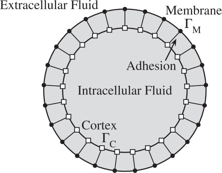
Model Components. Adhesion links the discretized cortex Γ_C (boxes) to the discretized cell membrane Γ_M (filled circles). Cytoplasmic fluid is located in the interior of the cell.

The cell membrane and cortex are modelled by active elastic structures. Forces arising from these structures drive fluid motion. The cell membrane moves with the fluid velocity, satisfying a no-slip condition. Because of the small length scales in the system, the Reynolds number is small, and the fluid equations are given by Stokes flow,

$$\begin{array}{r}\hfill \mu \mathrm{\Delta }\overrightarrow{u}-\nabla p+{\overrightarrow{f}}_{\text{M}}+{\overrightarrow{f}}_{\text{AD}}+{\overrightarrow{f}}_{\text{D}}=\overrightarrow{0},\\ \hfill \nabla \cdot \overrightarrow{u}=0.\end{array}$$ (1)

The variable u⃗ is the fluid velocity (μm/s), p is the pressure (g/μm s²) and μ is the dynamic viscosity of the fluid (P). The external fluid force densities (g/μm² s²) arise from membrane elasticity f⃗_M, membrane– cortex adhesion f⃗_AD and cortical drag f⃗_D.

The cortical velocity is determined by an additional balance of forces on the cortex. Myosin motors within the cortex generate active contractile tension. The other forces arise from adhesion to the membrane and drag from the background fluid. Because the cortex is modelled as a permeable elastic membrane, it moves with a velocity separate from the fluid velocity, which is determined by the force balance equation

$${\overrightarrow{F}}_{\text{D}}^{\text{C}}+{\overrightarrow{F}}_{\text{C}}^{\text{C}}+{\overrightarrow{F}}_{\text{AD}}^{\text{C}}=\overrightarrow{0}.$$ (2)

Each term has units of force per unit area (g μm⁻¹ s⁻²). The exact forms of each surface force density are provided later. Cortical forces are communicated to the fluid through drag and membrane–cortex adhesion forces.

The structures are represented by continuous 1D curves Γ_M (membrane) and Γ_C (cortex) immersed in a 2D fluid domain. Each curve is parameterized by reference arc length s, and their position is denoted by X⃗_M(s, t) (membrane) orX⃗_C(s, t) (cortex). We employ the immersed boundary formulation where structures are represented in a moving Lagrangian coordinate system, while fluid variables are located on a fixed Eulerian coordinate system (Peskin, 1977). We use this formulation because a moving Lagrangian coordinate system is a natural choice for representing deforming mechanical structures. Likewise, an Eulerian coordinate system is a natural choice for fluid variables. Also, the algorithm for communicating between coordinate systems is straightforward to implement. To distinguish between structure and fluid quantities, we use capital letters to indicate terms located on a structure and lower case letters for variables associated with the fluid. Additionally, superscripts indicate the location of the velocities and force densities, either membrane or cortex, i.e. the term ${\overrightarrow{U}}_{\text{F}}^{\text{C}}$ is the fluid velocity located on the cortex and ${\overrightarrow{F}}_{\text{AD}}^{\text{M}}$ represents adhesion force per unit area on the cell membrane. A surface force density on an immersed structure is spread onto the fluid coordinates as follows,

$$\overrightarrow{f}(\overrightarrow{x},t)=𝒮(\overrightarrow{F})={\int }_{\mathit{\Gamma }}\overrightarrow{F}(s,t)\delta (\overrightarrow{x}-\overrightarrow{X}(s,t))\text{d}s,$$ (3)

where δ(x⃗) is the 2D delta function. The notation 𝒮 indicates spreading the force per unit area from the Lagrangian (membrane) to force per unit volume in Eulerian (fluid) coordinates. The spreading operator conserves force, i.e.

$${\int }_{\mathit{\Gamma }}\overrightarrow{F}\text{d}S={\int }_{\mathit{\Omega }}𝒮(\overrightarrow{F})\text{d}\overrightarrow{x}.$$ (4)

We interpolate from Eulerian to Lagrangian coordinates to obtain fluid quantities. For example, to obtain the fluid velocity on Γ_M, we use the interpolation operator,

$${\overrightarrow{U}}_{\text{F}}^{\text{M}}={𝒮}_{\text{M}}^{*}(\overrightarrow{u})={\int }_{\mathit{\Omega }}\overrightarrow{u}(\overrightarrow{x},t)\delta (\overrightarrow{x}-\overrightarrow{X}(s,t))\text{d}\overrightarrow{x},$$ (5)

where Ω is the fluid domain.

Drag due to relative motion of the cortex is proportional to the difference between the cortical and fluid velocities, i.e.

$${\overrightarrow{F}}_{\text{D}}^{\text{C}}=\xi \left({\overrightarrow{U}}_{\text{F}}^{\text{C}}-{\overrightarrow{U}}_{\text{C}}\right),$$ (6)

where ξ is the drag coefficient (g μm⁻² s⁻¹). The drag coefficient is inversely proportional to the permeability of the cortex. We will explore this relationship more in Section 4. Because all the forces in the system sum to zero, drag on the cortex is equal and opposite to forces exerted on the fluid. The drag force density spread onto the Eulerian coordinates is denoted

$${\overrightarrow{f}}_{\text{D}}=-{𝒮}_{\text{C}}\left({\overrightarrow{F}}_{\text{D}}^{\text{C}}\right).$$ (7)

The cortex is modelled as a linear elastic material. At rest, it is under tension from actomyosin contractility. The cortex also experiences tension proportional to the amount it is stretched. The constitutive equation is given by,

$$T_{\text{C}}(s,t)={\gamma }_{\text{C}}+k_{\text{C}}\left(|\frac{\partial {\overrightarrow{X}}_{\text{C}}}{\partial s}|-1\right),$$ (8)

where γ_C (pN/μm) represents resting tension and k_C (pN/μm) is the cortical stiffness coefficient. The elastic modulus E_C is equal to k_C/ h, where h is the thickness of the cortex. We chose a reference arc length parameterization of the cortex so that |∂X⃗_C/∂s| is 1 when the cortex it is in its initial circular configuration.

A pure bilipid membrane cannot stretch. However, the cell membrane is a dynamic structure that flows, unfurls and exocytoses new material (Charras et al., 2008; Sheetz et al., 2006). For simplicity, we model the membrane as a linear elastic material. The implications of the membrane model are explored further in Section 4. The constitutive equation for membrane tension takes the same form as the equation for cortical tension in (8), i.e.

$$T_{\text{M}}(s,t)={\gamma }_{\text{M}}+k_{\text{M}}\left(|\frac{\partial {\overrightarrow{X}}_{\text{M}}}{\partial s}|-1\right),$$ (9)

where γ_M (pN/μm) is membrane tension is a resting configuration and k_M (pN/μm) is the stiffness coefficient. The value of |∂X⃗_M/∂s| is 1 when the membrane it is in its initial circular configuration because of the curve parameterization. The model parameters are further discussed in Section 4.

The force densities F⃗_C and F⃗_M generated by membrane and cortical tension are given by

$$\overrightarrow{F}=\frac{\partial }{\partial s}(T\overrightarrow{\tau }),$$ (10)

where the vector tangent to the membrane or cortex is

$$\overrightarrow{\tau }(s,t)=\frac{\partial \overrightarrow{X}/\partial s}{|\partial \overrightarrow{X}/\partial s|}.$$ (11)

Adhesion forces keep the membrane and cortex attached. This is modelled by discrete elastic springs connecting Γ_M to Γ_C (Fig. 1) with a stiffness coefficient k_AD (pN/μm³) and a resting length l_AD (μm), given by,

$$F_{\text{AD}}^{\text{M}}=-k_{\text{AD}}\left(\Vert {\overrightarrow{X}}_{\text{M}}-{\overrightarrow{X}}_{\text{C}}\Vert -l_{\text{AD}}\right)\frac{{\overrightarrow{X}}_{\text{M}}-{\overrightarrow{X}}_{\text{C}}}{\Vert {\overrightarrow{X}}_{\text{M}}-{\overrightarrow{X}}_{\text{C}}\Vert }.$$ (12)

The adhesion force density at a point on the cortex is equal and opposite to the force density at a corresponding point on the membrane,

$${\overrightarrow{F}}_{\text{AD}}^{\text{M}}+{\overrightarrow{F}}_{\text{AD}}^{\text{C}}=\overrightarrow{0}.$$ (13)

The spread adhesion force on the membrane in (1) is defined to be

$${\overrightarrow{f}}_{\text{AD}}=𝒮\left({\overrightarrow{F}}_{\text{AD}}^{\text{M}}\right).$$ (14)

3. Numerical formulation

The cell membrane and cortex are discretized on a moving Lagrangian grid parameterized by s. Each discretized boundary has N_b points with initial uniform mesh spacing Δs. Fluid quantities such as velocity and pressure are located on a fixed staggered Eulerian grid (Fig. 2). Periodic boundary conditions are used on the fluid domain because the flow outside of the cell is relatively stationary. Communication between grids is handled by the immersed boundary method (Peskin, 1977). To approximate the integrals in the spreading and interpolation operators (3–5), the delta function in one dimension is discretized as follows,

$$\delta (x)\approx {\delta }_{\mathrm{\Delta }x}(x)=\{\begin{array}{cc}\frac{1}{4\mathrm{\Delta }x}\left(1+\text{cos}\left(\frac{\pi x}{2\mathrm{\Delta }x}\right)\right),& \text{if}|x|<2\mathrm{\Delta }x\\ 0,& \text{otherwise.}\end{array}$$ (15)

where Δx is the spatial step size. In two dimensions, we have δ(x⃗) ≈ δ_Δx(x)δ_Δy(y). The discretization of the spreading operator (3) is

$${\overrightarrow{f}}_{i,j}^{n+1}=\mathrm{\Delta }s\sum _{k=1}^{N_b}{\overrightarrow{F}}_k^{n+1}{\delta }_{\mathrm{\Delta }x}\left(x_i-X_k^n\right){\delta }_{\mathrm{\Delta }y}\left(y_j-Y_k^n\right),$$ (16)

and the discrete interpolation operator (5) is given by,

$${\overrightarrow{U}}_k^{n+1}=\mathrm{\Delta }x\mathrm{\Delta }y\sum _{ij}{\overrightarrow{u}}_{i,j}^{n+1}{\delta }_{\mathrm{\Delta }x}\left(x_i-X_k^n\right){\delta }_{\mathrm{\Delta }y}\left(y_j-Y_k^n\right).$$ (17)

Fig. 2.

Staggered grid for fluid variables. The horizontal component of the velocity vector u is stored at filled squares. The vertical component υ is stored at circles. Pressure is stored at the centre of the computational cell, denoted by crosses.

At each time step, we solve for fluid velocity, pressure, external force densities, cortical velocity and positions of the membrane and cortex. Because the system has a large number of unknowns, and it is non-linear, we employ a fractional time stepping algorithm. The fractional time stepping that we use involves lagging the force densities in time. Force densities at the current time step are computed using the boundary configuration from the previous time step. Stokes equations (1) are then solved. Finally, immersed boundaries are updated with the appropriate fluid or cortical velocity.

Recall that the surface force density balance on the cortex is ${\overrightarrow{F}}_{\text{D}}^{\text{C}}+{\overrightarrow{F}}_{\text{C}}^{\text{C}}+{\overrightarrow{F}}_{\text{AD}}^{\text{C}}=\overrightarrow{0}$. Combining the previous equation with (7), the explicit fluid velocity dependence from the drag force density term in (1) is removed. The spread drag force then is

$${\overrightarrow{f}}_{\text{D}}={𝒮}_{\text{C}}\left({\overrightarrow{F}}_{\text{AD}}^{\text{C}}\right)+{𝒮}_{\text{C}}\left({\overrightarrow{F}}_{\text{C}}^{\text{C}}\right).$$ (18)

The fluid equation (1) becomes

$$\mu \mathrm{\Delta }\overrightarrow{u}-\nabla p+{𝒮}_{\text{M}}\left({\overrightarrow{F}}_{\text{M}}\right)+{𝒮}_{\text{M}}\left({\overrightarrow{F}}_{\text{AD}}^{\text{M}}\right)+{𝒮}_{\text{C}}\left({\overrightarrow{F}}_{\text{AD}}^{\text{C}}\right)+{𝒮}_{\text{C}}\left({\overrightarrow{F}}_{\text{C}}^{\text{C}}\right)=\overrightarrow{0}.$$ (19)

Because the above equation resembles that of forced Stokes flow, it is straightforward to solve. The update for the position of the cortex is

$$\frac{\text{d}{\overrightarrow{X}}_{\text{C}}}{\text{d}t}={\overrightarrow{U}}_{\text{C}}.$$ (20)

Combining the cortical surface force density balance (2) with the definition of the drag surface force density (6), we have

$${\overrightarrow{U}}_{\text{C}}={\overrightarrow{U}}_{\text{F}}^{\text{C}}+{\xi }^{-1}\left({\overrightarrow{F}}_{\text{C}}^{\text{C}}+{\overrightarrow{F}}_{\text{AD}}^{\text{C}}\right).$$ (21)

In this way, the cortical surface force density balance is used to update the position of the cortex. Equations (19) and (20) are solved in the algorithm described below.

The time stepping algorithm to update the system from tⁿ = nΔt to tⁿ⁺¹ is as follows:

1. Compute immersed boundary surface force densities F⃗_C, F⃗_M and F⃗_AD based on current membrane and cortex position. Derivatives are approximated with centred differences.

2. Spread the force densities onto nearby Eulerian points using (16).

3. Solve Stokes equations with external forces densities. For simplicity, the cytoplasmic fluid is taken to be equal to the extracellular fluid with viscosity μ. We take the divergence of (19) and solve a Poisson equation for the pressure p. Once the pressure is computed, we solve (19) for each velocity component u⃗ = (u, υ). Approximate the derivatives in Laplacian terms with centred differences, resulting in the standard five-point second-order Laplacian. Fast Fourier transforms are used to solve the Poisson equations.

4. Interpolate the fluid velocity to the membrane and cortex using (17).

5. Update the boundary positions with the appropriate velocities. The membrane update is

   $${\overrightarrow{X}}_{\text{M}}^{n+1}={\overrightarrow{X}}_{\text{M}}^n+\mathrm{\Delta }t{𝒮}_{\text{M}}^{*}\left({\overrightarrow{u}}^{n+1}\right)={\overrightarrow{X}}_{\text{M}}^n+\mathrm{\Delta }t{\overrightarrow{\mathit{U}}}_{\text{F}}^{n+1}.$$ (22)

The cortical update is

$${\overrightarrow{X}}_{\text{C}}^{n+1}={\overrightarrow{X}}_{\text{C}}^n+\mathrm{\Delta }t\left(\frac{1}{\xi }\left({\overrightarrow{F}}_{\text{C}}^{n+1}+{\overrightarrow{F}}_{\text{AD}}^{n+1}\right)+{𝒮}_{\text{C}}^{*}\left({\overrightarrow{u}}^{n+1}\right)\right).$$ (23)

4. Computational experiments

In this section, we begin by discussing the model parameters and the set-up of the computational experiments. Membrane and cortical elastic parameters are varied to determine their effect on steady state bleb size and shape. We then quantify bleb formation time and use this value to investigate the effects of varying cytoplasmic viscosity and drag over several orders of magnitude. We relate the drag coefficient in our model to permeability of the cortex and use this value to estimate the volume fraction of the cortex.

4.1. Parameters and simulation

A summary of model parameters from experimental data is listed in Table 1. The parameters for membrane and cortical tension are consistent with other studies (Charras et al., 2008). Note that measurements of viscosity and bleb formation time vary over several orders of magnitude. The cytoplasm is a complex material consisting of liquid cytosol, cytoskeleton, organelles and proteins. Experimental values of viscosity depend on the assumed cytoplasmic model. For example, an effective viscosity is a bulk measurement based on the viscosity of the liquid cytosol and cytoskeleton. However, in a poroelastic gel cytoplasmic model, the viscosity of the liquid cytosol without the cytoskeleton is reported, and this value is typically lower than an effective cytoplasmic viscosity (Charras et al., 2008; Keren et al., 2009). Later in this section, we vary the viscosity to determine the effect on bleb formation time.

Table 1.

Model parameters and sources

Symbol	Quantity	Value	Source
r M	Cell radius	10 μm	Tinevez et al. (2009)
γ M	Membrane surface tension	40 pN/μm	Tinevez et al. (2009)
k M	Membrane stiffness coefficient	4 pN/μm
r C	Cortex radius	9.0625 μm
γ C	Cortical tension	250 pN/μm	Tinevez et al. (2009)
k C	Cortical stiffness coefficient	100 pN/μm	Tinevez et al. (2009) Charras et al. (2005)
k AD	Adhesion stiffness coefficient	267 pN/μm3
l AD	0.001 μm
μ	Cytosolic viscosity	10−2–10 P	Kreis et al. (1982) Wirtz (2009)
ξ	Drag coefficient	10−2–101 g μm−2 s−1
−	Bleb formation time	5–30 s	Charras & Paluch (2008) Tinevez et al. (2009)
L	Fluid computational domain size	30 μm
Δx	Fluid grid step size	L/64
Δs	Initial structure grid step size	2πrΔx/(4L)

The cortex Γ_C and membrane Γ_M are initially circles parameterized by arc length in a reference configuration: Γ_C = r_C(cos(s/r_C), sin(s/r_C)) for 0 ⩽ s < 2πr_C and Γ_M = r_M(cos(s/r_M), sin(s/r_M)) for 0 ⩽ s < 2πr_M. The grid step size Δx used for most of the simulations in the following sections is 0.46875 μm (see Table 1). The distance between the membrane and cortex was chosen to be small but above grid scaling. We use the value of 0.9375 μm. This value is equal to 2Δx for the grid size listed in Table 1 where most of the results in this section are computed on.

At equilibrium, the cortical velocity and fluid velocity are both zero, and the membrane and cortex are stationary. From (21), adhesive force per unit area balances cortical force per unit area. Taking (21) in the normal direction to the cortex yields

$${\overrightarrow{F}}_{\text{AD}}^{\text{C}}\cdot \overrightarrow{n}+{\overrightarrow{F}}_{\text{C}}^{\text{C}}\cdot \overrightarrow{n}=k_{\text{AD}}\left(r_{\text{M}}-r_{\text{C}}-l_{\text{AD}}\right)-\frac{{\gamma }_{\text{C}}}{r_{\text{C}}}=0.$$ (24)

Substituting in the values for r_M, r_C, γ_C and the adhesion resting length l_AD = 0.001 μm, we obtain the stiffness coefficient for the adhesion force density, k_AD = 267 pN/μm³ from (24).

Before blebbing is initiated, the system is in equilibrium, and there is no fluid flow. Cortical tension due to actomyosin contractility is the dominant contributor in generating intracellular pressure. Forces from cortical tension are transmitted to the membrane through adhesion. Membrane–cortex adhesive forces balance forces from cortical contraction. Because the membrane is impermeable, forces from adhesion, membrane tension and cortical tension are balanced by internal pressure.

Blebbing is initiated by removing membrane–cortex adhesion in a small region as shown in Fig. 3. We chose the region to be from −π/32 < θ < π/32, corresponding to a bleb hole diameter of about 2 μm.

Fig. 3.

A bleb is initiated by removing membrane–cortex adhesion in a small region. The diameter of the bleb hole is about 2 μm.

Results from a simulation are shown in Fig. 4. Model parameters used in the simulation are listed in Table 1. The drag coefficient was set to 11 g μm⁻² s⁻¹ and the viscosity was set to 100 times the viscosity of water (1 P). After the adhesion is removed, forces from cortical tension are no longer transmitted to the membrane in a small region. As a result, pressure is reduced in a small area near the site of removed adhesion. This causes the cytoplasm to flow, expanding the membrane. Because the membrane is assumed to be a linear elastic material in our model, the bleb reaches a maximum steady state size when forces due to membrane elasticity balance the intracellular pressure. The process results in a new steady state membrane and cortex configuration (final time value in Fig. 4). The membrane and cortex stiffness coefficients play a large role in bleb size, which is investigated in the next section.

Fig. 4.

Colour field indicating pressure (Pa) with μ = 1 P and ξ = 11 g μm⁻² s⁻¹. Note that the initial pressure is lower across the cortex near the bleb nucleation site. The grid size used was 64 × 64.

4.2. Effects of membrane and cortical elasticity on bleb size

Experimental values of the elastic modulus of the cell cortex E_C have been reported to range from 34 Pa for alveolar epithelial cells (Laurent et al., 2002) to 2000 Pa for filamin-deficient M2 cells (Charras et al., 2005). Taking the cortical thickness to be 0.1 μm (Tinevez et al., 2009), the cortical stiffness coefficient k_C is equal to the elastic modulus times the cortical thickness and ranges from 3 to 200 pN/μm. There is no experimental value for the effective elastic modulus of the membrane that takes into account membrane unfurling, flow and exocytosis. Therefore, we simulated our model over a range of cortical elastic moduli and membrane stiffness coefficients to understand their contribution to bleb shape and expansion dynamics.

To quantify bleb size, we first measure cell width, which is defined to be the horizontal distance from the leftmost membrane point to the rightmost membrane point (Fig. 5). The initial cell diameter of 20 μm is then subtracted from the cell width to obtain bleb size. It should be noted that the leftmost membrane point moves less than 1% during the simulations presented in this section.

Fig. 5.

Cell width is defined to be the distance from the leftmost point on the membrane to the rightmost point. This value is subtracted from the initial cell diameter of 20 μm to give a measurement of bleb size. Bleb size reaches a steady state value that is used to measure bleb formation time.

Steady state bleb size as a function of membrane stiffness coefficient and cortical elastic modulus is listed in Table 2. Fluid viscosity was set to μ = 10 P and drag was ξ = 11 g μm⁻² s⁻¹. Additional parameters are listed in Table 1. The membrane did not achieve a steady state configuration for the (k_M, E_C) pairs of (2, 10), (2, 10^1.5) and (2, 10²). For these value pairs, intracellular pressure is above the threshold where membrane tension can resist bleb expansion (Tinevez et al., 2009). The steady state membrane configuration near the bleb is shown in Fig. 6. If the cortex is relatively soft, e.g. when E_C = 10 pN/μm², the bleb is relatively broad and does not achieve the circular shape observed experimentally. Above the value of k_M = 6 pN/μm, bleb size is about 1 μm. Thus, we chose k_M = 4 pN/μm and E_C = 1000 pN/μm² to obtain a bleb size of about 1 μm with a circular morphology.

TABLE 2.

Bleb size in micrometre as a function of cortical elastic modulus E_C = k_C/ h pN/μm² (h = cortical thickness) and membrane stiffness coefficient k_M pN/μm. Bold numbers indicate the values used for the remainder of the manuscript

Membrane stiffness coefficient (pN/μm2)	Cortical elastic modulus (pN/μm2)
	101	101.5	102	102.5	103	103.5	104
2	—	—	—	2.3	1.8	1.6	1.5
4	1.8	1.6	1.4	1.3	1.2	1.1	1.1
6	1.1	1.1	1.1	1.0	1.0	1.0	0.9
8	1.0	0.9	0.9	0.9	0.9	0.9	0.9
10	0.9	0.9	0.9	0.9	0.8	0.8	0.8

Fig. 6.

Steady state membrane configuration for several values of membrane stiffness coefficients and cortical elastic moduli.

4.3. Experiments on cytoplasmic viscosity and cortical drag

In this subsection, we present computational experiments to determine the relative roles of cytoplasmic viscosity and cortical drag on the dynamics of bleb formation. As previously mentioned, the viscosity of the cytoplasm can be interpreted differently depending on the underlying cytoplasmic model. In our model, the cytoplasm is modelled as a Newtonian fluid, and we interpret cytoplasmic viscosity to be a bulk effective viscosity. Experimental measurements for the effective viscosity of the cytoplasm vary over several orders of magnitude, ranging from 1 to 1000 times the viscosity of water (Kreis et al., 1982; Mastro et al., 1984; Wirtz, 2009). Cortical drag corresponds to permeability of the cortex. We explore this connection in detail in Section 4.4. The bleb formation timescale in our model is determined by the cortical drag coefficient and cytoplasmic viscosity. By analysing the viscosity–drag parameter space, we determine their relative roles in setting this timescale and identify the values of viscosity and drag that match experimentally measured bleb formation times.

We begin by quantifying the relative contribution of viscous and drag forces from the simulation shown in Fig. 4. We computed the ratio of the max norm of the viscous force density μΔu⃗ to the max norm of the drag force density f⃗_D. Figure 7 shows the norm of the viscous force density divided by the drag force density over time. Initially, the drag force density is about 30 times the viscous force density, then levels off at 200 times the viscous force density. Thus, we conclude drag forces dominate throughout this simulation.

Fig. 7.

Maximum norm of the viscous force density divided by the drag force density over time. Data are taken from the simulation in Fig. 4. Drag forces dominate viscous forces.

Before a thorough exploration of the viscosity–drag parameter space, we define how we quantify bleb formation time. The steady state shape is independent of the viscosity and drag and is determined only by the cortex and membrane stiffnesses. The viscosity and drag determine the dynamics of the approach to steady state. Figure 8 shows the time course of bleb size, as defined in Section 4.2, for several viscosity values with the drag coefficient set to 0.1 g μm⁻² s⁻¹. We define bleb formation time as the amount of time it takes for the bleb size to reach 90% of its steady state value.

Fig. 8.

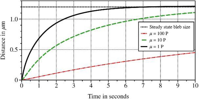
Time course of bleb size, as described in Section 4.2, for different viscosities and drag coefficient ξ = 0.1g μm⁻² s⁻¹. Bleb size approaches the steady state value of 1.2 μm indicated by the dotted line.

To determine the relative roles of drag and viscosity on bleb formation, we simulated our model for viscosities from 0.1 to 1000 P and drag coefficients from 10⁻² to 10 g μm⁻² s⁻¹. For each (μ, ξ) pair, we measured the time when bleb size reached 90% of the steady state bleb size of 1.2 μm. The results are shown in Fig. 9. Reported bleb formation times range from 5 to 30 s (Charras & Paluch, 2008; Tinevez et al., 2009). Taking the value of cytoplasmic viscosity to be 0.1–1 P (10–100 times more viscous than water), the drag coefficient must be larger than 1 g μm⁻² s⁻¹ to obtain experimentally measured bleb formation times. Additionally, Fig. 9 shows two regimes. For large viscosity and small drag coefficient values, bleb formation time depends only on cytoplasmic viscosity. For small viscosity and large drag coefficient values, cortical drag sets the timescale.

Fig. 9.

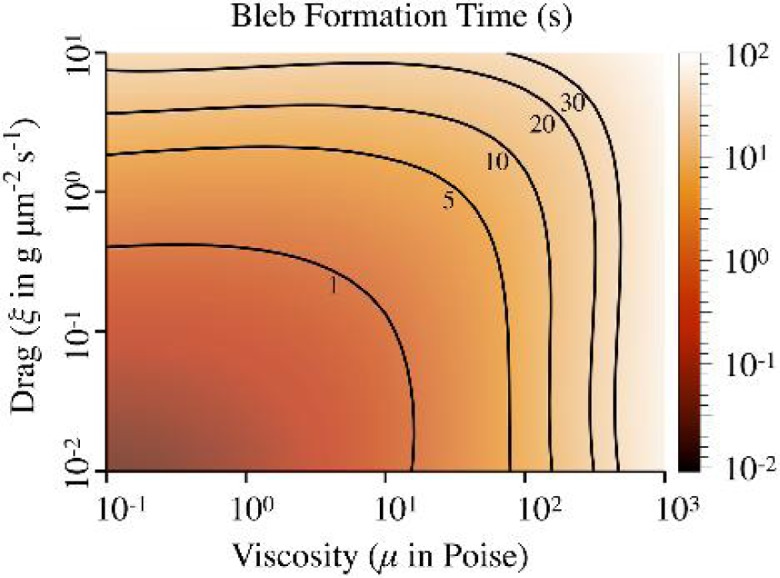
The colour field shows bleb formation times in seconds for different viscosity (P) and drag coefficient values (g μm⁻² s⁻¹). The solid contours indicate bleb formation times of 1, 5, 10, 20 and 30 s. The mesh was computed with cubic interpolation of the original data that consisted of 20 evenly spaced (μ, ξ) points from (10⁻¹, 10⁻²) to (10³, 10).

We verified our results with a convergence study on three grid refinements. The number of grid points on the three levels was N × N, with N = 64, 128 and 256. We used μ = 10 P and ξ = 1g μm⁻² s⁻¹. Bleb formation time varied by 6% from the N = 64 to 128 refinement and by 2% from N = 128 to 256 refinement. Our results are consistent with first-order convergence.

4.4. Interpretation of results

Another way to interpret the drag coefficient is to relate it to the permeability of the cortex. Flow through a porous medium is described by Darcy’s law (Bear, 1972)

$$U_p=\frac{k[p]}{\mu a},$$ (25)

where U_p (μm/s) is the porous slip velocity, [p](g μm⁻¹s⁻²) is the pressure jump, k (μm²) is the permeability of the material and a (μm) is the thickness of the material. In our model, the force density balance on the cortex is

$$\xi \left({\overrightarrow{U}}_{\text{C}}-{\overrightarrow{U}}_{\text{C}}^{\text{C}}\right)={\overrightarrow{F}}_C^C+{\overrightarrow{F}}_{\text{AD}}^{\text{C}}.$$ (26)

The porous slip velocity is

$$U_p=\left({\overrightarrow{U}}_{\text{C}}-{\overrightarrow{U}}_{\text{F}}^{\text{C}}\right)\cdot \overrightarrow{n}=F_n/\xi ,$$ (27)

where F_n is the normal component of the cortical force density. From (25) and (27), the expression for the permeability of the cortex is

$$k=\frac{\mu a{F}_n}{\xi [p]}.$$ (28)

The jump in the normal fluid stress across the cortex generates a jump in the pressure of [p] = F_n|∂X⃗_C/∂s| (Kim & Peskin, 2006; Stockie, 2009). Therefore, the permeability in terms of our model parameters is

$$k=\frac{\mu a}{\xi |\partial {\overrightarrow{X}}_{\text{C}}/\partial s|}.$$ (29)

We take |∂X⃗_C/∂s| to be its initial value of 1. Cortical thickness a is 0.1 μm (Tinevez et al., 2009). We let the value of cytoplasmic viscosity μ be 0.1 P (Charras et al., 2008). In our computational experiments, the drag coefficient ξ varies from 10⁻² to 10 g μm²s⁻¹ (Table 1 and Fig. 9). Plugging the values of |∂X⃗_C/∂s|, a, μ and the range of ξ into (29), the resulting permeability k varies from 10⁻⁷ to 10⁻² μm². We found large drag values match experimental bleb formation times for μ = 0.1 P. Using the value of ξ = 10 g μm² s⁻¹, the corresponding permeability estimate is on the order of k = 10⁻⁷ μm². Our prediction for the permeability of the cortex is in line with experimentally measured biological materials. For example, the permeability of water through collagen fibres with radius 10⁻³μm and a volume fraction of 0.215 is 5 × 10⁻⁷μm² (Jackson & James, 1986).

Cytoplasmic permeability has been estimated in other contexts. In the lamellipodium of a keratocyte, permeability was estimated to be 10⁻³ μm² in Keren et al. (2009). The cytoplasmic permeability throughout the cell was estimated at 10⁻⁴ μm² in Charras et al. (2008). Both these estimates assume the intracellular cytoplasm is a porous medium, whereas in our model, all drag is located at the cortex. This might explain why the permeability estimates in Charras et al. (2008) and Keren et al. (2009) are larger.

We also calculate the volume fraction in the cortex using our estimate for permeability. An analytic formula for the permeability of rods randomly oriented in three dimensions was given in Spielman & Goren (1968),

$$\frac{1}{\varphi }=\frac{4}{3}+\frac{10}{3}\frac{\sqrt{k}}{\lambda }\frac{K_1(\lambda /\sqrt{k})}{K_0(\lambda /\sqrt{k})},$$ (30)

where ϕ is the volume fraction, λ is the radius of the fibres and K₀ and K₁ are modified Bessel functions of the zeroth and first kind, respectively. It should be noted that this formula is consistent with the experimentally measured collagen permeability and volume fraction data mentioned in the previous paragraph. In our case, we take λ to be the radius of an actin bundle, which we estimate to be 10⁻² μm. Taking k = 10⁻⁷ μm², we obtain the volume fraction ϕ = 0.7 from (30). Equation (30) is highly sensitive to the choice of λ. Ifwetake λ to be the radius of an actin monomer, about 10⁻³ μm, then the volume fraction drops to ϕ = 0.39. We estimate the volume fraction of the cortex to be a range from 0.4 to 0.7. This is the first estimate for the volume fraction of the cortex. The range of predicted cortical volume fractions is high, but it is in agreement with other estimates. For example, the volume fraction of cytoskeleton throughout the cell was estimated to be 0.8 in Charras et al. (2008) and 0.5 in a keratocyte lamellipodium (Keren et al., 2009).

Average pore size can be computed from volume fraction. In Chatterjee (2010), a formula relating average pore size 〈r〉 to volume fraction ϕ is presented for the case of a spatially uniform and randomly oriented network of cylindrical fibres with radius λ,

$$\langle r\rangle =\frac{\lambda }{2}\sqrt{\frac{\pi }{\alpha }}{\text{e}}^{\alpha }(\text{erf}(1-\sqrt{\alpha })),$$ (31)

where α = ln (1/(1 − ϕ)) and erf is the error function. Taking ϕ = 0.7 from the previous volume fraction calculation, average pore size is about 1/3 times the fibre radius or 3 nm if λ = 10⁻² μm. Typical cortical pore sizes are reported from 20 to 200 nm in Charras et al. (2006). These numbers are based on images from scanning electron microscopy. The pore size appears to be comparable to the fibre size in these images (Fig. 6 in Charras et al., 2006). One likely reason for our underestimate of the average pore size is that we consider average pore size. Larger pores are easier to visualize and quantify in the microscopy images. It is more difficult to obtain a mean pore size. Additionally, our low estimate of pore size may result from the assumption that the drag force is localized to the cortex. If the drag force inside the cell due to cytoskeleton and organelles is included, this may predict a higher cortical permeability and a larger pore size. Internal cytoskeleton could be included in this modelling framework, but such an extension is non-trivial and beyond the scope of the current work.

5. Discussion

We have presented a computational model of bleb formation that includes the cytoplasm, cell membrane, cortex and adhesion between the membrane and cortex. A novel feature of our model is that the cortex is treated as a porous elastic structure that moves with a separate velocity due to drag between the cortex and cytoplasmic fluid. The role of the cortical elastic modulus and membrane stiffness coefficient on bleb shape and steady state times was investigated. We measured bleb formation time over a range of values in the drag–viscosity parameter space because the timescale of bleb formation is set by these parameters in our model. We identified two regimes. Viscosity dominates the dynamics in one regime and drag plays a significant role in the other. A typical value for cytoplasmic viscosity is 10 times the viscosity of water (0.1 P) (Charras et al., 2008; Keren et al., 2009). Using this value, we calculated the permeability to be 10⁻⁷ μm² and a range of volume fractions of the cortex from 0.4 to 0.7. These values suggest that the cortex is tightly packed with a gap size about one third the size of the fibre radius. Experimental evidence suggests that the gap size is larger and volume fraction is smaller. In our model, intracellular drag is attributed to the cortex. Other factors such as the drag on the internal cytoskeleton may contribute to bleb dynamics.

The computational model presented here is a 2D model. Because the dynamics are determined by flow through the cortex and membrane expansion, we do not expect that the time and bleb size scales would substantially change from those computed by a 3D model. In our simulations, blebbing was initiated by removing adhesion between the membrane and the cortex. If blebbing was initiated by ablating the cortex, there may be significant differences 2D and 3D models. The elastic stresses near a cut in a circular membrane may be very different from the stresses around a hole in a spherical membrane. However, a 2D model facilitates rapid parameter studies that would be be computationally expensive in a 3D model. The data from this study give us a starting point for more detailed quantitative computational experiments with a 3D model.

Experiments show that secondary blebs are slightly smaller than the primary bleb (Tinevez et al., 2009). In our model, multiple blebs are all the same size (data not shown). This is because not much pressure is relieved by bleb expansion. It is not known what relieves intracellular pressure. One hypothesis is that internal compression of the cytoskeleton plays a significant role (Tinevez et al., 2009). Our model can be extended to quantify the contributions of cytoskeletal compressibility and internal drag on bleb dynamics by treating the material on the inside of the cell as poroelastic. This will be the subject of future work.

Our approach to incorporating porosity into the immersed boundary method is different from previous work. In Kim & Peskin (2006) and Stockie (2009), the porous slip velocity is proportional to the immersed boundary force density in the normal direction. In our model, we have two force density balances. One from the fluid equation and one on the cell cortex. The force density balance on the cortex determines the porous slip velocity, which allows for slip in the tangential direction.

The model presented here is a first step towards understanding the dynamics of blebbing, which is particularly important for understanding 3D cell motility. An advantage of using the immersed boundary method is that it is straightforward to add additional components to the model, such as cytoplasmic elasticity and sub-cellular structures. The framework of our model allows for future explorations on the role of these structures in blebbing and in intracellular pressure propagation.

References

- Alberts B, Johnson A, Lewis J, Raff M, Roberts K, Walter P. Molecular Biology of the Cell. 4th edn. New York: Garland Science; 2002. [Google Scholar]
- Bear J. Dynamics of Fluids in Porous Media. New York: Dover; 1972. [Google Scholar]
- Charras G, Paluch E. Blebs lead the way: how to migrate without lamellipodia. Nat Rev Mol Cell Biol. 2008;9:730–736. doi: 10.1038/nrm2453. [DOI] [PubMed] [Google Scholar]
- Charras GT, Coughlin M, Mitchison TJ, Mahadevan L. Life and times of a cellular bleb. Biophys J. 2008;94:1836–1853. doi: 10.1529/biophysj.107.113605. [DOI] [PMC free article] [PubMed] [Google Scholar]
- Charras GT, Hu CK, Coughlin M, Mitchison TJ. Reassembly of contractile actin cortex in cell blebs. J Cell Biol. 2006;175:477–490. doi: 10.1083/jcb.200602085. [DOI] [PMC free article] [PubMed] [Google Scholar]
- Charras GT, Yarrow JC, Horton MA, Mahadevan L, Mitchison TJ. Non-equilibration of hydrostatic pressure in blebbing cells. Nature. 2005;435:365–369. doi: 10.1038/nature03550. [DOI] [PMC free article] [PubMed] [Google Scholar]
- Chatterjee AP. Nonuniform fiber networks and fiber-based composites: pore size distributions and elastic moduli. J Appl Phys. 2010;108:063 513. [Google Scholar]
- Erickson CA, Trinkaus JP. Microvilli and blebs as sources of reserve surface membrane during cell spreading. Exp Cell Res. 1976;99:375–384. doi: 10.1016/0014-4827(76)90595-4. [DOI] [PubMed] [Google Scholar]
- Fackler OT, Grosse R. Cell motility through plasma membrane blebbing. J Cell Biol. 2008;181:879–884. doi: 10.1083/jcb.200802081. [DOI] [PMC free article] [PubMed] [Google Scholar]
- Fishkind DJ, Cao LG, Wang YL. Microinjection of the catalytic fragment of myosin light chain kinase into dividing cells: effects on mitosis and cytokinesis. J Cell Biol. 1991;114:967–975. doi: 10.1083/jcb.114.5.967. [DOI] [PMC free article] [PubMed] [Google Scholar]
- Jackson G, James D. The permeability of fibrous porous-media. Can J Chem Eng. 1986;64:364–374. [Google Scholar]
- Keren K, Yam PT, Kinkhabwala A, Mogilner A, Theriot JA. Intracellular fluid flow in rapidly moving cells. Nat Cell Biol. 2009;11:1219–1224. doi: 10.1038/ncb1965. [DOI] [PMC free article] [PubMed] [Google Scholar]
- Kim Y, Peskin CS. 2-D parachute simulation by the immersed boundary method. SIAM J Sci Comput. 2006;28:2294–2312. [Google Scholar]
- Kreis TE, Geiger B, Schlessinger J. Mobility of microinjected rhodamine actin within living chicken gizzard cells determined by fluorescence photobleaching recovery. Cell. 1982;29:835–845. doi: 10.1016/0092-8674(82)90445-7. [DOI] [PubMed] [Google Scholar]
- Laurent VM, Hénon S, Planus E, Fodil R, Balland M, Isabey D, Gallet F. Assessment of mechanical properties of adherent living cells by bead micromanipulation: comparison of magnetic twisting cytometry vs optical tweezers. J Biomech Eng. 2002;124:408–421. doi: 10.1115/1.1485285. [DOI] [PubMed] [Google Scholar]
- Mastro AM, Babich MA, Taylor WD, Keith AD. Diffusion of a small molecule in the cytoplasm of mammalian cells. Proc Natl Acad Sci USA. 1984;81:3414–3418. doi: 10.1073/pnas.81.11.3414. [DOI] [PMC free article] [PubMed] [Google Scholar]
- Mills JC, Stone NL, Erhardt J, Pittman RN. Apoptotic membrane blebbing is regulated by myosin light chain phosphorylation. J Cell Biol. 1998;140:627–636. doi: 10.1083/jcb.140.3.627. [DOI] [PMC free article] [PubMed] [Google Scholar]
- Peskin CS. Numerical analysis of blood flow in the heart. J Comput Phys. 1977;25:220–252. [Google Scholar]
- Sheetz MP, Sable JE, Döbereiner HG. Continuous membrane-cytoskeleton adhesion requires continuous accommodation to lipid and cytoskeleton dynamics. Annu Rev Bioph Biom. 2006;35:417–434. doi: 10.1146/annurev.biophys.35.040405.102017. [DOI] [PubMed] [Google Scholar]
- Spielman L, Goren SL. Model for predicting pressure drop and filtration efficiency in fibrous media. Environ Sci Technol. 1968;2:279–287. [Google Scholar]
- Stockie JM. Modelling and simulation of porous immersed boundaries. Comput Struct. 2009;87:701–709. [Google Scholar]
- Tinevez JY, Schulze U, Salbreux G, Roensch J, Joanny JF, Paluch E. Role of cortical tension in bleb growth. Proc Natl Acad Sci USA. 2009;106:18581–18586. doi: 10.1073/pnas.0903353106. [DOI] [PMC free article] [PubMed] [Google Scholar]
- Wirtz D. Particle-tracking microrheology of living cells: principles and applications. Annu Rev Biophys. 2009;38:301–326. doi: 10.1146/annurev.biophys.050708.133724. [DOI] [PubMed] [Google Scholar]
- Wolf K, Mazo I, Leung H, Engelke K, von Andrian UH, Deryugina EI, Strongin AY, Bröcker EB, Friedl P. Compensation mechanism in tumor cell migration: mesenchymal-amoeboid transition after blocking of pericellular proteolysis. J Cell Biol. 2003;160:267–277. doi: 10.1083/jcb.200209006. [DOI] [PMC free article] [PubMed] [Google Scholar]
- Young J, Mitran S. A numerical model of cellular blebbing: a volume-conserving, fluid-structure interaction model of the entire cell. J Biomech. 2010;43:210–220. doi: 10.1016/j.jbiomech.2009.09.025. [DOI] [PMC free article] [PubMed] [Google Scholar]
Associated Data
This section collects any data citations, data availability statements, or supplementary materials included in this article.