Kinesins with Extended Neck Linkers: A Chemomechanical Model for Variable-Length Stepping

Abstract

We develop a stochastic model for variable-length stepping of kinesins engineered with extended neck linkers. This requires that we consider the separation in microtubule binding sites between the heads of the motor at the beginning of a step. We show that this separation is stationary and can be included in the calculation of standard experimental quantities. We also develop a corresponding matrix computational framework for conducting computer experiments. Our matrix approach is more efficient computationally than large-scale Monte Carlo simulation. This efficiency greatly eases sensitivity analysis, an important feature when there is considerable uncertainty in the physical parameters of the system. We demonstrate the application and effectiveness of our approach by showing that the worm-like chain model for the neck linker can explain recently published experimental data. While we have focused on a particular scenario for kinesins, these methods could also be applied to myosin and other processive motors.

1 Introduction

Kinesin motor proteins use the energy of ATP hydrolysis to transport intracellular cargo along microtubules. Plus-ended kinesins are typically dimeric, containing two “heads” or motor domains, each of which binds ATP and microtubules. The heads are connected by their flexible neck linker domains to a coiled-coil stalk that terminates in a cargo-binding tail domain (Fig. 1). A wild-type dimeric kinesin uses its two heads to step along a microtubule, transporting vesicles, protein complexes, and other cargo to the periphery of the cell. Since the repeat distance of a tubulin dimer is 8 nm, each step results in an 8-nm displacement of the motor.

Fig. 1.

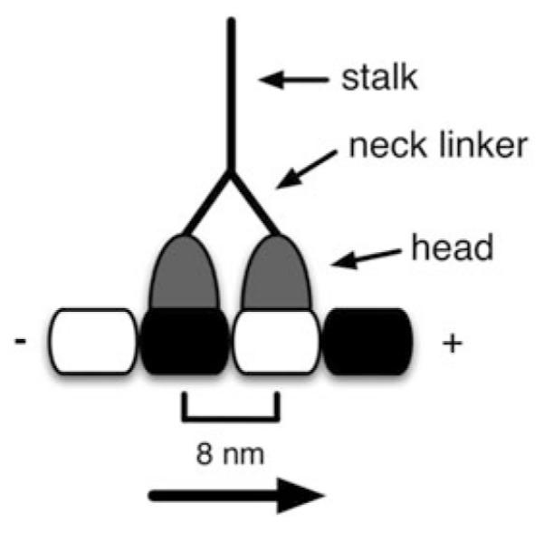
The gross anatomy of a kinesin motor protein

The molecular mechanism by which kinesins step along microtubules has been the subject of intense investigation using biophysical and biochemical assays as well as analytical and computational modeling. The mechanism is described as a “hand over hand” cycle (Hackney et al. 2003; Vale and Milligan 2000; Block 2007) during which each head alternately binds, undergoes a conformational change, and detaches from the microtubule. Kinesin is a processive motor, which is to say that a kinesin takes multiple (~100) 8-nm steps per interaction with a microtubule. Processivity requires coordination in the chemomechanical cycle of the two motor domains such that at least one head is attached to the microtubule at all times. The ability to move processively involves both precise coordination between the chemomechanical cycles in each motor domain and mechanical communication between the motor domains to properly synchronize their ATP hydrolysis cycles.

The neck linker domain, a 14 amino acid sequence that has a contour length of ~5 nm, is a key structural element of kinesin. The neck linker domain has at least three distinct roles: (1) as the motor steps along the microtubule, the neck linker docks to the core motor domain, producing a plus-end displacement of a few nanometers toward the next binding site on the microtubule; (2) following neck linker docking, the free head diffuses to its next binding site, tethered by its neck linker domain; and (3) when the tethered head binds, generating a strained two-head bound state, mechanical forces between the two heads that underlie head–head coordination are transmitted through the neck linker domain. Hence, the neck linker must properly dock to the head; it must be sufficiently compliant to allow tethered diffusion of the free head, yet sufficiently stiff to relay the forces between the heads.

To experimentally test neck linker function, a number of groups have generated kinesins with extended neck linkers and measured the resulting change in the biochemical or transport characteristics of the motors. Hackney found that extending the neck linker up to 12 residues had little effect on the maximal ATPase of the motor but decreased the biochemical processivity approximately twofold. Muthukrishnan et al. (2009) and Shastry and Hancock (2010) found that extending the Kinesin-1 neck linker by only a few amino acids significantly reduced motor run lengths (mechanical processivity). Yildiz et al. (2008) engineered up to 26 proline residues into the neck linker of human Kinesin-1 and measured the speed, run length, and various other characteristics of the mutant motors. They found that speed decreased markedly with increasing neck linker length while run length exhibited little or no decrease, and with increasing neck linker length the motors took larger forward steps as well as backward steps. From these studies it is clear that the mechanical properties of the neck linker domain play a key role in the efficient stepping of kinesin, but quantifying how extending the neck linker alters docking, diffusive tethering, and inter-head force transmission is difficult without an integrated analytical or computational model of kinesin stepping.

Mathematical models for kinesin and other linear processive molecular motors generally fall into a few categories. (See Julicher et al. 1997; Kolomeisky and Fisher 2007; Mogilner et al. 2002 for reviews.) First, there are purely kinetic models that represent the chemical states necessary for the motor to step. These models typically consist of a periodic discrete-space Markov chain where a return to a particular state corresponds to a single physical step of the motor (Hackney et al. 2003; Gilbert et al. 1995; Muthukrishnan et al. 2009; Shastry and Hancock 2010). However, during a mechanical step, the motor must move continuously through space, a fact that leads to an alternative description of the motor as a Brownian particle in a periodic potential. The chemical state of the motor can be incorporated using a flashing ratchet model that employs a stochastic differential equation for the position of the motor, where the drift is modulated by the current chemical state.

The difficulty with these standard formulations is that they provide a general description of the “position” of the motor instead of explicitly describing the dynamics of each motor head. To understand the neck linker extension experiments described in the biophysical literature, it is important to consider the diffusional dynamics of the tethered free head of the motor. There are a few examples of previous modeling efforts that do consider the movements of the free head. For example, Mather and Fox (2006) included tethered diffusion in an analytical model of kinesin stepping that posited irreversible binding exclusively to the forward binding site, and Atzberger and Peskin (2006) created a three-dimensional model of the tethered diffusion of the free head. In previous work by two of the current authors and Kutys et al. (2010) we integrated a Brownian dynamics model of tethered head diffusion into a stochastic model of the kinesin hydrolysis cycle. While this model was useful for analyzing the importance of neck linker mechanics on the diffusional search of the tethered head for the next binding site, it was rather computationally expensive and did not lend itself to detailed sensitivity analysis.

We recently formulated a model for the uniform-length stepping of kinesins—a model that accounts explicitly for the constrained diffusion of the free head—and developed a corresponding matrix computational framework for conducting sensitivity analyses (Hughes et al. 2011). Modeling the individual heads of a kinesin allows for the analysis of motors with extended neck linker domains and permits the comparison of competing models for neck linker dynamics. However, this model had a limitation in that it could handle only kinesins that exhibit uniform-length stepping. Furthermore, the model incorporated inter-head tension only implicitly through static rate constants.

It has been shown experimentally that a kinesin with a sufficiently long neck linker is capable of taking steps of varying lengths (variable-length stepping) including backward steps (Yildiz et al. 2008). After the motor takes a large step, the tension between the heads, which is dictated by the properties of the neck linker domain, will be larger, resulting in different kinetic rate constants than for uniform-length stepping. While the previous model for neck linker extension (Hughes et al. 2011) was insufficient for describing variable-length stepping, there have been previous examples of variable-length stepping especially when considering myosin motors. Specifically, Kolomeisky and coauthors have explored variable-length stepping by a modification of a finite-state periodic model that allows for closed-form solutions (Das and Kolomeisky 2008; Kolomeisky and Fisher 2003). In addition, these previous works have incorporated explicit spatial forces that could include the effect of a freely diffusing head. Other models that incorporated variable-length stepping includes Shaevitz et al. (2005), who explored variable-length stepping by analyzing the step-time distribution. The present method differs by handling a relatively more complex model of the constrained diffusion of the free head at the expense of the explicit formulas found in this previous work. As both myosin and dynein naturally take variable-length steps, there is a broad need for this type of model to properly interpret single-molecule experimental data (Mallik et al. 2004; Rock et al. 2001).

In this paper, we extend our previous model for uniform-length stepping to handle variable-step kinesins, and we describe a simple yet powerful framework for quickly conducting in silico experiments similar to the laboratory experiment of Yildiz et al. (2008). Our computational scheme is applied to kinesins with neck linker inserts ranging from six to 26 prolines, using two competing physical models for mechanical properties of the neck linker. To compare with experimental results, motor velocity, run length, and effective diffusion are computed, along with an analysis of the distribution of step sizes for different neck-linker-extended motors. The models are first run without considering the change in inter-head tension that results from variable-length steps. Then, the change in tension is modeled explicitly using a Boltzmann factor, similar to the method for incorporating the effect of the cargo on a stepping motor in Chen et al. (2002).

We will present a detailed model of a variable-length step cycle, link this model to the stepping, and show the effects of different neck linker models on standard experimental quantities. Section 2 will present a model for the constrained diffusion of the freely diffusing head coupled to the kinetic state which occurs within one cycle. This within-step model will depend on the separation between the heads of the motor at the end of the previous cycle and will terminate after the head which has become free then reattaches. In Sect. 3, we will review a framework for stepping models previously introduced in Hughes et al. (2011) that will allow us to connect the within-step model to the overall dynamics of the motor along the microtubule. In Sect. 4, we discuss a concrete computational strategy to evaluate experimental quantities by linking our local diffusive model to the variable-length stepping of kinesins. In Sect. 5, we demonstrate our method for explaining the data from Yildiz et al. (2008).

The results of the paper can be summarized as follows.

• – We construct a local within-step model for kinesin which takes into account the dynamics of the individual heads and allows for variable-length stepping.

• – We formulate a semi-Markov model for stepping to calculate important experimental quantities and link this scale to the local within-step model.

• – We compare competing models for the kinesin neck linker.

• – We conclude that a worm-like chain model for the neck linker combined with detachment rates that consider tension between the heads best matches the relevant experiments in the literature.

2 Within-Step Dynamic Model

In general, a motor model should include not only chemical transitions but also diffusion of the free head during a step of the motor. We now present a within-step model for which a cycle comprises detachment of one head, the tethered diffusion of that free head, and eventual rebinding of the head while also tracking the chemical states of the motor. This model was previously explored using stochastic simulation methods (Kutys et al. 2010) and further developed in Hughes et al. (2011); however, in these previous presentations, the motor was only permitted to step to neighboring binding sites.

Assume first that the front head is bound at location 0. If the initial number of binding sites separating the heads is S* and the rear head detaches, the free head will have an initial position of y = –L · S* (where L is the distance nanometers (nm) between binding sites), but the position of the head will immediately begin to fluctuate due to Brownian forces. We model the fluctuating position of the free head using a stochastic differential equation with a drift that is determined by the nature of the neck linker tether connecting the diffusing head to the bound head. The position of the free head is thus governed by the following equation:

$$Y\left(t\right)=y+{\int }_0^t{a}_{K\left(s\right)}\left(Y\right(s\left)\right)\mathit{ds}+\sigma B\left(t\right),$$ (1)

where K(t) is the discrete-state Markov chain corresponding to chemical state of the motor described in more detail below, and B(t) is a standard Brownian motion. The drift, a_K(·), is determined by the nature of the neck linker and the location of the bound head. The drift can be thought of as the instantaneous mean velocity of the free head. A relatively straightforward example for the drift can be derived from the potential energy corresponding to a Hookean spring connecting the free head to the bound head. In this case, a_K(y) = –κ(y – y₀)/ζ, where K is the chemical state, y₀ is an offset, κ is the spring constant, and ζ is the drag coefficient.

The process K(t) represents the chemical state of the motor at time t. For the purposes of the current discussion, we will be considering four chemical states. The first state is when both heads of the kinesin are bound to the microtubule. The second state describes rear head detachment from the microtubule. The third state corresponds to ATP binding, and the fourth state describes ATP hydrolysis. An appropriate way to think of the process K(t) then is as a discrete-space Markov chain including transitions between these four states. We will need to augment this number of states in subsequent sections to describe other aspects of the models, such as the varying distance between the heads at the initial time and whether the front head or rear head detached from the microtubule.

When a motor head is near a binding site, an exponential clock will be started where the rate may depend on the proximity of the head to the binding site. Each binding site has an independent clock. If the clock is triggered, the motor binds to that site. This model then describes the movements of the free head of the kinesin motor in one cycle given the distance between the bound heads at the beginning of a cycle. We consider one cycle to start when both heads are bound. We define the length of a step to be the change in position of the front head from the end of one cycle to the end of the next. We will only refer to the heads as the front and rear heads when the motor has both of the heads bound to the microtubule.

The transition rates between relevant chemical states may not always be homogeneous with respect to the location of the free head. The binding processes could be written as

$$A_j\left(t\right)=N_j\left({\int }_0^t{g}_j\left(Y\right(s\left)\right)\mathit{ds}\right),$$ (2)

where the N_j are independent standard Poisson processes (also independent of B). The index j corresponds to a possible binding site, and the function g_j(·) is a local binding rate for site j that depends on the position of the free head, Y(t). In general, for a particular position, Y(t), only one of the functions, g_j(Y(t)), will be nonzero. One possible selection of the g_j(·) would be a scaled indicator function on some neighborhood of the binding site. Another possibility would be a function that increased to a maximum at the binding site. Note that this is equivalent to modeling the time to absorption in state j as an independent random variable, τ_j, when conditioned on the process Y as

$$\mathbb{P}({\tau }_j>t)=\exp \left(-{\int }_0^t{g}_j\left(Y\right(s\left)\right)\mathit{ds}\right).$$ (3)

The time to binding is then defined as

$$\tau =\inf \{t:A_j(t)>0\text{for some}j\}.$$ (4)

We also define Y(τ) to be the location of the free head at the end of a cycle. In Sect. 4, we will incorporate the chemical model and the diffusion model in an illustrative example for variable-step motors. A simpler SDE model would assume that this binding time is a hitting time, so that the probability of a step with a given length is merely the probability of arriving at the appropriate binding site. However, considering the true three-dimensional geometry, this may not be reasonable, and so we establish this probability of binding when the motor is within a certain radius of the binding site. Moreover, a hitting time formulation would not allow for variable-length stepping.

In the next section, we will present a stepping model. If we can calculate the first and second moments for the duration of a cycle, the first and second moments for the length of a step, and the covariance between the two, we will be able to link this within-step model to a stepping model and calculate important experimental quantities such as asymptotic velocity and effective diffusion. We will need to consider the distance between the heads at the end of each cycle in order to determine the initial conditions for the next cycle in this variable-length stepping scenario.

3 Stepping Models for Kinesin

In this section, we review the framework from our previous work (Hughes et al. 2011) for a uniform-step motor, a motor capable of stepping forward or backward by only one binding site, and we define important quantities of interest in the study of molecular motors. In particular, we see that the asymptotic velocity and effective diffusion are natural descriptions of a coarsened version of kinesin stepping. We will present run length as a measure of processivity of a motor and will then expand on this model to incorporate a variable-length step.

3.1 Review of Uniform-Length Stepping

We begin by introducing some notation and then recall some facts from our uniform-step framework (Hughes et al. 2011). We let N(t) denote the number of steps taken up to time t, τ_i denote the time required to take the ith step, and Z_i denote the size in microtubule binding sites of the ith step as an integer number of tubulin subunits (each spaced 8 nm apart). In the case of uniform-length stepping, each step has the same initial condition: both heads are bound, and one binding site separates them. Consequently, the time and size of the current step do not depend on those of the preceding step or any previous step. In other words, the sequence {(τ_i, Z_i)}_i≥1 is independent and identically distributed. Given this assumption, N(t) is an example of a renewal process with the τ_i called renewals. Since {(τ_i, Z_i)}_i≥1 are identically distributed, we assume the τ_i have finite mean μ_τ and finite variance ${\sigma }_{\tau }^2$, the Z_i have finite mean μ_Z and finite variance ${\sigma }_Z^2$, and that their covariance is σ_Z,τ.

Two important quantities in the study of molecular motors depend on the position of the motor at time t, which can be expressed as

$$X\left(t\right)=L\sum _{i=1}^{N\left(t\right)}{Z}_i,$$ (5)

where L is the distance between binding sites. The first of these quantities is asymptotic velocity, which can be defined as

$$V_{\infty }=\underset{t\to \infty }{\lim }\frac{\mathbb{E}X\left(t\right)}{t}.$$ (6)

Given the above definition of X(t), we apply some standard features of renewal processes to obtain

$$V_{\infty }=\underset{t\to \infty }{\lim }\frac{\mathbb{E}L{\Sigma }_{i=1}^{N\left(t\right)}{Z}_i}{t}=L\frac{{\mu }_Z}{{\mu }_{\tau }}.$$ (7)

In addition to these properties of the expectation of the process, one may verify a strong law of large numbers,

$$V_{\infty }=\underset{t\to \infty }{\lim }\frac{X\left(t\right)}{t}=\underset{t\to \infty }{\lim }\frac{L{\sum }_{i=1}^{N\left(t\right)}{Z}_i}{t}=L\frac{{\mu }_Z}{{\mu }_{\tau }},$$ (8)

a useful fact for data analysis. This implies that the empirical velocity for the path of one motor will converge to the asymptotic velocity.

A second quantity of interest is effective diffusion (Mogilner et al. 2002), which can be defined as

$$D=\underset{t\to \infty }{\lim }\frac{\mathbb{V}X\left(t\right)}{2t}.$$ (9)

In Hughes et al. (2011), we were able to apply a functional central limit theorem from Whitt (2002), which relies on a central limit theorem for the partial sums ∑Z_i and ∑τ_i. Using a scaling parameter n,

$$n^{-1∕2}\left(X\right(\mathit{nt})-V_{\infty }\mathit{nt})\Rightarrow \sqrt{2D}B\left(t\right)$$

as n → ∞, where B(t) is a standard Brownian motion, and

$$D=\frac{L^2}{2}\left(\frac{{\mu }_Z^2{\sigma }_{\tau }^2}{{\mu }_{\tau }^3}+\frac{{\sigma }_Z^2}{{\mu }_{\tau }}-2\frac{{\mu }_Z{\sigma }_{Z,\tau }}{{\mu }_{\tau }^2}\right)=(V_{\infty }^2{\sigma }_{\tau }^2+L^2{\sigma }_Z^2-2L{V}_{\infty }{\sigma }_{Z,\tau })∕\left(2{\mu }_{\tau }\right).$$ (10)

Note that this also implies a more traditional central limit theorem for the quantity

$$2D{t}^{-1∕2}\left(X\right(t)-V_{\infty }t),$$

which converges to a standard normal random variable as time increases.

We also consider processivity through the expected run length of a motor—how far a motor travels on average before dissociation. This quantity is commonly used in experimental settings (Block et al. 1990; Vale et al. 1996). It is natural to model the number of steps prior to dissociation as a random variable, N. The distance traveled before detachment is then given by

$$R=L\sum _{i=1}^N{Z}_i.$$ (11)

Using this definition, the mean run length is

$$\mathbb{E}R=L\mathbb{E}N\mathbb{E}{Z}_i=L\frac{{\mu }_Z}{r},$$ (12)

where r is the probability of becoming detached at any time step i. Note that the processivity is defined in a slightly different framework as the asymptotic quantities. However, both of these quantities, asymptotic and detachment-based, appear in the experimental literature and can be though of as reasonable approximations if the motors take many steps before detachment.

3.2 Variable-Length Stepping

Our within-step model is a local model in the sense that we focus on the dynamics within a single step, the events that occur between two successive bindings to the microtubule. In the uniform-length stepping scenario, the neck linkers are long enough to permit the free head to rebind at only two locations, the binding sites on either side of the bound head. Thus, the separation between the heads at the end of a step—and consequently the initial separation for the next cycle—is always one binding site. Since the initial condition is the same for each step, the within-step dynamics are identical and require no information from the previous step. So, the steps are independent. An illustration of uniform-length stepping is shown in Fig. 2, where Z is the step size. We define Z to be the binding site location occupied by the front head at the end of a step minus the binding site location occupied by the front head at the beginning of the step, where “front” means closest to the plus end of the microtubule.

Fig. 2.

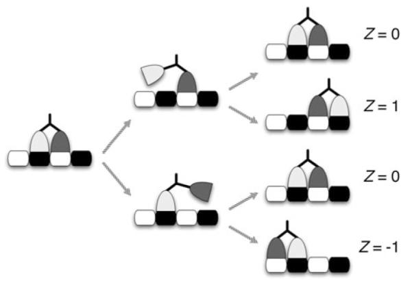
An illustration of uniform-length stepping

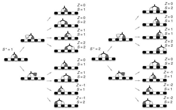
The initial condition for a motor with extended neck linkers, on the other hand, may vary depending on the previous step. For example, a motor with neck linkers twice as long as those of a wild-type motor can reach four binding sites, two on either side of the bound head, which implies that the ending separation between heads, call it S, is either one or two binding sites. Hence, the initial separation, S*, for the next step will also be one or two sites. The stepping of such a motor is illustrated in Fig. 3.

Fig. 3.

An illustration of variable-length stepping for a motor with neck linkers long enough to permit a separation of two binding sites. S* is the initial separation of the heads, S is the final separation, and Z is the step size

The first panel of the figure shows the possible outcomes, (Z, S), for S* = 1, and the second panel shows possibilities given S* = 2. In the sequel, we will discuss in some detail the transition from the (i – 1)th step = of the chain to the ith step. To simplify notation, we will use a superscript * to indicate the (i – 1)th cycle and no superscript to indicate the ith cycle.

Since variable-length steps are not identical, the ending separation for a given step becomes the initial separation for the next step, which implies that adjacent steps are not independent. In the previous uniform-step framework, we needed to consider only the moments of step duration and step direction. Now we must also consider the separation between heads when both heads are bound. Fortunately, this sequence, {S_i}_i>1, of separations forms a Markov chain. Moreover, the distribution of the duration of the ith cycle, τ, and the length of the ith step, Z, will depend on the previous cycle only through the separation between the heads at the end of the previous cycle, S*, greatly aiding computation. To generalize the formulas from the previous section for velocity and diffusion, we need to verify that the sum of the Markov chain {(S_i, τ_i, Z_i)}_i>1 will converge under the appropriate scaling to a normal random vector. If this can be verified, and if the mean vector and covariance matrix can be calculated, we will be able to use (7) and (10) to calculate the effective diffusion and asymptotic velocity.

We will continue to be primarily interested in the position process

$$X\left(t\right)=\sum _{i=1}^{N\left(t\right)}{Z}_i,$$ (13)

and this is one element of a semi-Markov process. In general, a semi-Markov process is defined as a stochastic process on the nonnegative reals that jumps at discrete times and the time between jumps and the value of the process during that epoch form a Markov chain. Thus, the framework presented here is a multivariate semi-Markov process with time between events equal to τ_i and the value of the process on the ith interval equal to (S_i, Z_i, ${\sum }_{j=1}^i$ Z_j). We are only interested in the final component of the process. Semi-Markov chains were previously explored as a model for related biophysical phenomena in Wang and Qian (2007).

In the next section, we will describe two specific variable-length stepping models and corresponding computations. To set the stage for those discussions, we will complete this section by stating assumptions and defining notation that is relevant for applying our framework in the context of any specific stepping model. We assume that {(S_i, τ_i, Z_i)}_i>1 has a stationary distribution, which must satisfy

$$\pi (s,t,z)={\int }_0^{\infty }\sum _{z^{\ast }}\sum _{s^{\ast }}p(s,t,z\mid s^{\ast },t^{\ast },z^{\ast })\pi (s^{\ast },t^{\ast },z^{\ast }){\mathit{dt}}^{\ast },$$ (14)

where p(·|·) denotes the one-step transition density. Assume further that the transition density depends only on the separation of the heads at the beginning of the cycle, S*. Then

$$\pi (s,t,z)=\sum _{s^{\ast }}p(s,t,z\mid s^{\ast }){\pi }_S\left(s^{\ast }\right),$$ (15)

where π_S is the stationary density of {S_i}_i>1. If we can calculate this stationary distribution, we can use (15) to find the stationary distribution of the full three-dimensional process.

Now we introduce some notation to simplify the sequel. First, let the first moment, second moment, and variance of τ with respect to the stationary distribution be denoted by ${\mu }_{\tau }={\mathbb{E}}_{\pi }\tau ,{\eta }_{\tau }={\mathbb{E}}_{\pi }{\tau }^2$, and ${\sigma }_{\tau }^2={\eta }_{\tau }-{\mu }_{\tau }^2$. And let the conditional moments of τ given the value of the initial separation, S*, be denoted by μ^τ|S* and η_τ|S*. To organize the calculations, we will form vectors μ_τ|S* and η_τ|S* over all possible values of the initial separation. We use similar notation for the moments of Z: μ_Z, η_Z, ${\sigma }_Z^2$, μ_Z|S*, η_Z|S*, μ_Z|S*, and η_Z|S*. We will also require the conditional probabilities for Z and S given S*; the simplest way to organize these calculations is in matrices which we denote by P_Z|S* and P_S|S*, respectively. More specifically,

$${\mathbf{P}}_{Z\mid S^{\ast }}=\left(\begin{array}{ccc}\hfill \mathbb{P}(Z=0\mid S^{\ast }=1)\hfill & \hfill \dots \hfill & \hfill \mathbb{P}(Z=s^{\max }\mid S^{\ast }=1)\hfill \\ \hfill ⋮\hfill & \hfill \ddots \hfill & \hfill ⋮\hfill \\ \hfill \mathbb{P}(Z=0\mid S^{\ast }=s^{\max })\hfill & \hfill \dots \hfill & \hfill \mathbb{P}(Z=s^{\max }\mid S^{\ast }=s^{\max })\hfill \end{array}\right)$$ (16)

where s^max is the maximum possible separation of the two heads when both are bound, i.e., S* ∈ {1, 2, … , s^max}, which implies that Z ∈ {0, ±1, … , s^max}. Note that P_S|S* is the standard probability transition matrix for {S_i}_i≥1.

For computation of the unconditional moments, we assume that {_Si}_i≥1 has a stationary distribution, the pmf of which we represent as the vector ${\pi }_S={\left(\mathbb{P}\right(S=1),\dots ,\mathbb{P}(S=s^{\max }\left)\right)}^{\prime }$. Note that π_S is the principal right eigenvector of P’_S|S*, the eigenvector associated with eigenvalue 1. Now, if we let z be the vector of possible step lengths, we have

$${\mu }_{\tau }={\mathbb{E}}_{\pi }\tau =\sum _{s^{\ast }}{\int }_0^{\infty }\mathit{tp}(t\mid s^{\ast }){\pi }_S\left(s^{\ast }\right)={\mu }_{\tau \mid S^{\ast }}^{\prime }{\pi }_S,$$ (17)

$$\begin{array}{cc}\hfill {\mu }_Z& =\sum _z\sum _s\sum _{s^{\ast }}\mathit{zp}(s,z,\mid s^{\ast }){\pi }_S\left(s^{\ast }\right)=\sum _{s^{\ast }}\sum _z\mathit{zp}(z\mid s^{\ast }){\pi }_S\left(s^{\ast }\right)\hfill \\ \hfill & =z^{\prime }{{\mathbf{P}}^{\prime }}_{Z\mid S^{\ast }}{\pi }_S={{\mu }^{\prime }}_{Z\mid S^{\ast }}{\pi }_S.\hfill \end{array}$$ (18)

Similarly, ${\sigma }_{\tau }^2={\eta }_{\tau \mid S^{\ast }}^{\prime }{\pi }_S-{\mu }_{\tau }^2$ and ${\sigma }_Z^2=z_2^{\prime }{{\mathbf{P}}^{\prime }}_{Z\mid S^{\ast }}{\pi }_S={{\eta }^{\prime }}_{Z\mid S^{\ast }}{\pi }_S-{\mu }_Z^2$, where z₂ = z ● z, with ● denoting row-wise multiplication (vector–vector or matrix–vector). And for the covariance, σ_Z,τ = μ’_Zτ|S*π_S – μ_Zμ_τ.

The above notation and formulas will allow us to decompose relevant calculations into those involving only the process {S_i}_i≥1 and those involving (τ, Z) given the separation in the previous cycle. To summarize, we will need to calculate

• – the stationary distribution for {S_i}_i≥1

• – the first and second moments of the conditional distribution p(z, t|s*).

In the next section, we illustrate these calculations for two relevant models.

4 Connecting the Within-Step Model to the Stepping Model

We now illustrate how to make the necessary calculations to obtain the asymptotic velocity and effective diffusion for two examples of variable-length stepping models. The first, a purely kinetic model, is primarily for illustrative purposes. The second corresponds to the model described in Sect. 2, which includes both diffusive and kinetic components.

4.1 Purely Chemical Model

A common motor model assumes that a motor must pass through a sequence of chemical states in order to take a step (Hancock and Kinesin 2003; Block 2007; Vale and Milligan 2000; Schief and Howard 2001; Cross 2004). A simple example of such a model is shown in Fig. 4. We use this chemical model to create a continuous-time discrete-state Markov chain, Y(t), that corresponds to a within-step model for the motor. The chain starts in chemical state 1 and evolves until absorbed in one of nine absorbing states corresponding to one of the outcomes shown in Fig. 3. We use the transition rate matrix for the chain to compute the moments of τ and Z, which are in turn used to compute the quantities of interest introduced in Sect. 3.

Fig. 4.

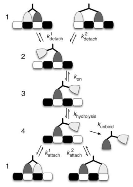
A chemical model for variable-length stepping. For this model, the maximum separation of the heads is two binding sites, and so this chemical model corresponds to the stepping diagrammed in Fig. 3. Note that k_on corresponds to the binding of one molecule of ATP

One way to describe the transition rate matrix, Q, for Y(t) is to use the block form

$$\mathbf{Q}\left(S^{\ast }\right)=\left(\begin{array}{cc}\hfill \mathbf{A}\left(S^{\ast }\right)\hfill & \hfill \mathbf{B}\left(S^{\ast }\right)\hfill \\ \hfill 0\hfill & \hfill 0\hfill \end{array}\right),$$ (19)

where A represents the evolution within the step, B includes the transitions to the absorbing states, and S* ∈ {1, 2}. The 0 matrices are included to ensure that Q is square. Specifically, for the chemical cycle shown in Fig. 4, A and B will be defined as

$$\mathbf{A}\left(S^{\ast }\right)=\left(\begin{array}{ccccccc}\hfill k_{1,1}\hfill & \hfill k_{1,2_{\mathrm{R}}}\hfill & \hfill 0\hfill & \hfill 0\hfill & \hfill k_{1,4_{\mathrm{F}}}\hfill & \hfill 0\hfill & \hfill 0\hfill \\ \hfill 0\hfill & \hfill k_{2_{\mathrm{R}},2_{\mathrm{R}}}\hfill & \hfill k_{2_R,3_{\mathrm{R}}}\hfill & \hfill 0\hfill & \hfill 0\hfill & \hfill 0\hfill & \hfill 0\hfill \\ \hfill 0\hfill & \hfill k_{3_{\mathrm{R}},2_{\mathrm{R}}}\hfill & \hfill k_{3_{\mathrm{R}},3_{\mathrm{R}}}\hfill & \hfill k_{3_R,4_{\mathrm{R}}}\hfill & \hfill 0\hfill & \hfill 0\hfill & \hfill 0\hfill \\ \hfill 0\hfill & \hfill 0\hfill & \hfill k_{4_{\mathrm{R}},3_{\mathrm{R}}}\hfill & \hfill k_{4_{\mathrm{R}},4_{\mathrm{R}}}\hfill & \hfill 0\hfill & \hfill 0\hfill & \hfill 0\hfill \\ \hfill 0\hfill & \hfill 0\hfill & \hfill 0\hfill & \hfill 0\hfill & \hfill k_{4_{\mathrm{F}},4_{\mathrm{F}}}\hfill & \hfill k_{4_{\mathrm{F},}{3}_{\mathrm{F}}}\hfill & \hfill 0\hfill \\ \hfill 0\hfill & \hfill 0\hfill & \hfill 0\hfill & \hfill 0\hfill & \hfill k_{3_{\mathrm{F}},4_{\mathrm{F}}}\hfill & \hfill k_{3_{\mathrm{F}},3_{\mathrm{F}}}\hfill & \hfill k_{3_{\mathrm{F}},2_{\mathrm{F}}}\hfill \\ \hfill 0\hfill & \hfill 0\hfill & \hfill 0\hfill & \hfill 0\hfill & \hfill 0\hfill & \hfill k_{2_{\mathrm{F}},3_{\mathrm{F}}}\hfill & \hfill k_{2_{\mathrm{F}},2_{\mathrm{F}}}\hfill \end{array}\right)$$ (20)

and

$$\begin{array}{cc}\hfill \mathbf{B}& \left(S^{\ast }\right)\hfill \\ \hfill =& \left(\begin{array}{ccccccccc}\hfill 0\hfill & \hfill 0\hfill & \hfill 0\hfill & \hfill 0\hfill & \hfill 0\hfill & \hfill 0\hfill & \hfill 0\hfill & \hfill 0\hfill & \hfill 0\hfill \\ \hfill k_{2_{\mathrm{R}},1_1^0}\hfill & \hfill k_{2_{\mathrm{R}},1_2^0}\hfill & \hfill 0\hfill & \hfill 0\hfill & \hfill 0\hfill & \hfill 0\hfill & \hfill 0\hfill & \hfill 0\hfill & \hfill 0\hfill \\ \hfill 0\hfill & \hfill 0\hfill & \hfill 0\hfill & \hfill 0\hfill & \hfill 0\hfill & \hfill 0\hfill & \hfill 0\hfill & \hfill 0\hfill & \hfill 0\hfill \\ \hfill 0\hfill & \hfill 0\hfill & \hfill 0\hfill & \hfill 0\hfill & \hfill k_{4_{\mathrm{R}},1_1^1}\hfill & \hfill 0\hfill & \hfill 0\hfill & \hfill 0\hfill & \hfill k_{4_{\mathrm{R}},1_2^2}\hfill \\ \hfill k_{4_{\mathrm{F}},1_1^0}\hfill & \hfill k_{4_{\mathrm{F}},1_2^0}\hfill & \hfill k_{4_{\mathrm{F}},1_1^{-1}}\hfill & \hfill 0\hfill & \hfill 0\hfill & \hfill k_{4_{\mathrm{F}},1_2^1}\hfill & \hfill 0\hfill & \hfill 0\hfill & \hfill 0\hfill \\ \hfill 0\hfill & \hfill 0\hfill & \hfill 0\hfill & \hfill 0\hfill & \hfill 0\hfill & \hfill 0\hfill & \hfill 0\hfill & \hfill 0\hfill & \hfill 0\hfill \\ \hfill 0\hfill & \hfill 0\hfill & \hfill k_{2_{\mathrm{F}},1_1^{-1}}\hfill & \hfill k_{2_{\mathrm{F}},1_2^{-1}}\hfill & \hfill 0\hfill & \hfill 0\hfill & \hfill k_{2_{\mathrm{F}},1_1^{-2}}\hfill & \hfill k_{2_{\mathrm{F}},1_2^{-2}}\hfill & \hfill 0\hfill \end{array}\right),\hfill \end{array}$$ (21)

where R and F represent rear head detachment and front head detachment, respectively. Note that k_i,i will be the negated sum of the nondiagonal entries of the ith row of A and the entries of the ith row of B. Note that the values of these rates can be filled in from Table 1.

Table 1.

Default parameter values. Note that k_on depends on the concentration of ATP. Specifically, we are assuming that $k_{\text{on}}=k_{\text{on}}^{\mathrm{ATP}}$[ATP], where $k_{\text{on}}^{\mathrm{ATP}}$ and [ATP] = 1000 μM. The notation k’ denotes the reverse kinetic rate corresponding to k

Parameter	Default value
κ (FENE)	0.1 pN/nm
ζ	5.66 × 10−8 pNs/nm
σ 2	1.46 × 108 nm2 s−1
Binding radius	1 nm
kattach (WLC)	180,000 s−1
kattach (FENE)	2,800 s−1
$k_{\text{attach}}^{\prime }$	2,500
$k_{\text{detach}}^{\prime }$	0.1 s−1
k on	2,000 s−1
$k_{\text{on}}^{\prime }$	200 s−1
k hydrolysis	280 s−1
$k_{\text{hydrolysis}}^{\prime }$	3.5 s−1
k unbind	1.7 s−1

The nine columns of B correspond to steps of length 0, 0, −1, −1, 1, 1, −2, −2, and 2, respectively. Except for a step of size 2, there are two columns for a given step size, z. The first column corresponds to a final separation of 1 binding site, and the second column to a final separation of 2 binding sites. And so a given ending state, $1_s^z$, corresponds to returning to chemical state 1 such that Z = z and S = s. Note that there is only one column for Z = 2 because the event (Z = 2, S = 1) is impossible. And some of the rates shown in B will be 0 for a given S*. For example, $k_{4_{\mathrm{F}}{1}_1^{-1}}=0$ when S* = 1 because Z = −1 is not possible then.

While the matrix B shown above was constructed based on the various possibilities for (Z, S) enumerated in Fig. 3, we could instead formulate B using a spatial grid of microtubule binding sites like that shown in Fig. 5, where we assume that the front head is located at binding site 0 at the beginning of a cycle. In this scheme, the binding site for the detached head determines Z and S. The resulting matrix is given by

$$\mathbf{B}\left({\mathit{S}}^{\ast }\right)=\left({\mathbf{B}}_{\mathrm{R}}\right({\mathit{S}}^{\ast }\left){\mathbf{B}}_{\mathrm{F}}\right({\mathit{S}}^{\ast }\left)\right),$$ (22)

where

$${\mathbf{B}}_{\mathrm{R}}\left(S^{\ast }\right)=\left(\begin{array}{ccccccc}\hfill -4\hfill & \hfill -3\hfill & \hfill -2\hfill & \hfill -1\hfill & \hfill 0\hfill & \hfill 1\hfill & \hfill 2\hfill \\ \hfill 0\hfill & \hfill 0\hfill & \hfill 0\hfill & \hfill 0\hfill & \hfill 0\hfill & \hfill 0\hfill & \hfill 0\hfill \\ \hfill 0\hfill & \hfill 0\hfill & \hfill k_{2_{\mathrm{R}},1_2^0}\hfill & \hfill k_{2_{\mathrm{R}},1_1^0}\hfill & \hfill 0\hfill & \hfill 0\hfill & \hfill 0\hfill \\ \hfill 0\hfill & \hfill 0\hfill & \hfill 0\hfill & \hfill 0\hfill & \hfill 0\hfill & \hfill 0\hfill & \hfill 0\hfill \\ \hfill 0\hfill & \hfill 0\hfill & \hfill 0\hfill & \hfill 0\hfill & \hfill 0\hfill & \hfill k_{4_{\mathrm{R}},1_1^1}\hfill & \hfill k_{4_{\mathrm{R}},1_2^2}\hfill \\ \hfill 0\hfill & \hfill 0\hfill & \hfill 0\hfill & \hfill 0\hfill & \hfill 0\hfill & \hfill 0\hfill & \hfill 0\hfill \\ \hfill 0\hfill & \hfill 0\hfill & \hfill 0\hfill & \hfill 0\hfill & \hfill 0\hfill & \hfill 0\hfill & \hfill 0\hfill \\ \hfill 0\hfill & \hfill 0\hfill & \hfill 0\hfill & \hfill 0\hfill & \hfill 0\hfill & \hfill 0\hfill & \hfill 0\hfill \end{array}\right)$$ (23)

and

$${\mathbf{B}}_{\mathrm{F}}\left(S^{\ast }\right)=\left(\begin{array}{ccccccc}\hfill -4\hfill & \hfill -3\hfill & \hfill -2\hfill & \hfill -1\hfill & \hfill 0\hfill & \hfill 1\hfill & \hfill 2\hfill \\ \hfill 0\hfill & \hfill 0\hfill & \hfill 0\hfill & \hfill 0\hfill & \hfill 0\hfill & \hfill 0\hfill & \hfill 0\hfill \\ \hfill 0\hfill & \hfill 0\hfill & \hfill 0\hfill & \hfill 0\hfill & \hfill 0\hfill & \hfill 0\hfill & \hfill 0\hfill \\ \hfill 0\hfill & \hfill 0\hfill & \hfill 0\hfill & \hfill 0\hfill & \hfill 0\hfill & \hfill 0\hfill & \hfill 0\hfill \\ \hfill 0\hfill & \hfill 0\hfill & \hfill 0\hfill & \hfill 0\hfill & \hfill 0\hfill & \hfill 0\hfill & \hfill 0\hfill \\ \hfill 0\hfill & \hfill 0\hfill & \hfill 0\hfill & \hfill k_{4_{\mathrm{F}}{1}_1^{-1}}\hfill & \hfill k_{4_{\mathrm{F}},1_1^0:1_2^0}\hfill & \hfill k_{4_{\mathrm{F}},1_1^2}\hfill & \hfill 0\hfill \\ \hfill 0\hfill & \hfill 0\hfill & \hfill 0\hfill & \hfill 0\hfill & \hfill 0\hfill & \hfill 0\hfill & \hfill 0\hfill \\ \hfill k_{2_{\mathrm{F}},1_2^{-2}}\hfill & \hfill k_{2_F,1_2^{-1}:1_1^{-2}}\hfill & \hfill k_{2_{\mathrm{F}},1_1^{-1}}\hfill & \hfill 0\hfill & \hfill 0\hfill & \hfill 0\hfill & \hfill 0\hfill \end{array}\right)$$ (24)

Now each column corresponds to a binding site, and the rates in a given column correspond to absorptions such that the detached head rebinds at the given site. We need two replications of the grid in order to keep track of which head detached. Note that two elements of the matrix show two rates, one for S* = 1 and the other for S* = 2.

Fig. 5.

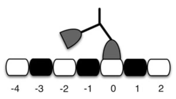
The grid of numbered binding sites used to devise the second version of the B matrix

Now that we have formulated the A and B matrices given the value of the initial separation; we can use them to compute the various probabilities and moments given in the previous section—and, consequently, V_∞, D, and $\mathbb{E}$R—as follows. Our formulation allows us to write down a distribution for the duration of a step, the time required for Y(t) to reach an absorbing state after having left state 1. See Hughes et al. (2011) for a more detailed derivation of results that follow. The cumulative distribution function for τ is given by

$$F\left(t\right)=1-{\mathit{a}}^{\prime }{e}^{\mathbf{A}t}1,$$ (25)

where the vector a has a 1 in the first location and the value 0 elsewhere, and 1 is a conformable vector of 1s. And so the corresponding density is

$$f\left(t\right)=-{\mathit{a}}^{\prime }\mathbf{A}{e}^{\mathbf{A}t}1.$$ (26)

Hence, the conditional first and second moments of τ are given by

$${\mu }_{\tau \mid S^{\ast }}=-{\mathit{a}}^{\prime }{\left[\mathbf{A}\right(s^{\ast }\left)\right]}^{-1}1,$$ (27)

$${\eta }_{\tau \mid S^{\ast }}=2{\mathit{a}}^{\prime }{\left[\mathbf{A}\right(s^{\ast }\left)\right]}^{-2}1.$$ (28)

To calculate the conditional moments of Z given S*, we need P_z|s*. To compute a given entry in this matrix, $\mathbb{P}(Z=z\mid S^{\ast }=s^{\ast })$, we construct a vector, c, that contains value 1 in the locations corresponding to step size z. Using c, we can compute the relevant probability as

$$\mathbb{P}(Z=z\mid S^{\ast }=s^{\ast })=-{\mathit{a}}^{\prime }{\left[\mathbf{A}\right(s^{\ast }\left)\right]}^{-1}\mathbf{B}\left(s^{\ast }\right)\mathit{c}.$$ (29)

Finally, the conditional cross moment is given by μ_Zτ|S* = a’[A(s*)⁻²B(s*)z, where the vector z contains the possible values of Z. In the context of our example model, z = (0, 0, −1, −1, 1, 1, −2, −2, 2)’ for the first version of B.

We can compute the probability transition matrix for {S}_i≥1, which we call P_S|S*, in the same way we computed P_Z|S*, the only difference being that c must now mark the locations corresponding to the desired ending separation.

It is important to note that this type of model can be handled by previous computational methods. Due to the quasi-periodic nature of the underlying kinetic model, one could, for example, modify the methods of Das and Kolomeisky (2003, 2008) similar to the modification of the Wang, Peskin, and Elston method found in Fricks et al. (2005, 2006). However, we are taking a conceptually different approach by stopping the local Markov chain corresponding to the within-step model after the free head becomes rebound; this has the advantage of allowing either the front or rear head to become initially unbound. Thus, the conditions for the computations to be successful are that the matrix A(s*) be invertible for each relevant s* and for the Markov chain {S}_i≥1 to have a unique stationary distribution. Since the transition probabilities for the Markov chain are derived from the computation, this is checked numerically. We have included pseudocode and more details about the computation in Appendices A and B.

4.2 Including Tethered Diffusion

We have now presented a computational framework for handling variable-step kinesins when only a kinetic model is considered. However, our goal is to include the constrained diffusion of the free head along with transitions in the chemical state of the motor. To accomplish this, we will create a discrete-space approximating Markov chain for the diffusive part of the within-step model presented in Sect. 2, Y(t), and couple this to the chemical kinetic process, K(t), through a block structure for the rate matrix. This formulation is closely related to the computational approach presented in Hughes et al. (2011) but is modified here to include variable-length steps and the effect of such stepping on the following cycle.

Assume that y₁, … , y_n is an evenly spaced grid on the real line with a distance between grid points of Δ. We represent an approximating Markov chain for dY(t) = a(Y(t))dt + σ(Y(t))dB(t) using the tridiagonal transition matrix, L, with elements

$$\begin{array}{cc}\hfill {\mathbf{L}}_{i,i-1}=& \left(\frac{{\sigma }^2\left(\mathit{yi}\right)}{2}+a^{-}\left(\mathit{yi}\right)\Delta \right)/{\Delta }^2,\hfill \\ \hfill {\mathbf{L}}_{i,i+1}=& \left(\frac{{\sigma }^2\left(\mathit{yi}\right)}{2}+a^{+}\left(\mathit{yi}\right)\Delta \right)/{\Delta }^2,\hfill \\ \hfill {\mathbf{L}}_{i,j}=& 0\text{if}\mid i-j\mid >1,\hfill \\ \hfill {\mathbf{L}}_{i,i}=& -({\mathbf{L}}_{i,i-1}+{\mathbf{L}}_{i,i+1}),\hfill \end{array}$$ (30)

where a(y) = a⁺(y) – a⁻(y) is the drift, and σ(y) is the diffusion coefficient, which should be constant in this case of Brownian diffusion in a potential. We use the approximating Markov chain rates found in Kushner and Dupuis (2001), but there are alternatives including one commonly used for motor models, the WPE method (Wang et al. 2003).

We would like to incorporate this model of diffusion into a computational framework that also includes chemical transitions; within each chemical state, the diffusion will be determined by a particular drift function, a_k(y). Thus, we construct an approximating chain for {(Y(t), K(t))} by using a block structure. The “outer” structure will describe the discrete chemical reactions, and the “inner” structure will represent the diffusive component of our model. The outer form, which is quite similar to the matrices given above for the purely kinetic model, is as follows:

$$\mathbf{A}=\mathbf{A}\left(S^{\ast }\right)=\left(\begin{array}{ccccccc}\hfill {\mathbf{K}}_{1,1}\hfill & \hfill {\mathbf{K}}_{1,2_{\mathrm{R}}}\hfill & \hfill 0\hfill & \hfill 0\hfill & \hfill {\mathbf{K}}_{1,4_{\mathrm{F}}}\hfill & \hfill 0\hfill & \hfill 0\hfill \\ \hfill 0\hfill & \hfill {\mathbf{K}}_{2_{\mathrm{R}},2_{\mathrm{R}}}\hfill & \hfill {\mathbf{K}}_{2_{\mathrm{R}},3_{\mathrm{R}}}\hfill & \hfill 0\hfill & \hfill 0\hfill & \hfill 0\hfill & \hfill 0\hfill \\ \hfill 0\hfill & \hfill {\mathbf{K}}_{3_{\mathrm{R}},2_{\mathrm{R}}}\hfill & \hfill {\mathbf{K}}_{3_{\mathrm{R}},3_{\mathrm{R}}}\hfill & \hfill {\mathbf{K}}_{3_{\mathrm{R}},4_{\mathrm{R}}}\hfill & \hfill 0\hfill & \hfill 0\hfill & \hfill 0\hfill \\ \hfill 0\hfill & \hfill 0\hfill & \hfill {\mathbf{K}}_{4_{\mathrm{R}},3_{\mathrm{R}}}\hfill & \hfill {\mathbf{K}}_{4_{\mathrm{R}},4_{\mathrm{R}}}\hfill & \hfill 0\hfill & \hfill 0\hfill & \hfill 0\hfill \\ \hfill 0\hfill & \hfill 0\hfill & \hfill 0\hfill & \hfill 0\hfill & \hfill {\mathbf{K}}_{4_{\mathrm{F}},4_{\mathrm{F}}}\hfill & \hfill {\mathbf{K}}_{4_{\mathrm{F}},3_{\mathrm{F}}}\hfill & \hfill 0\hfill \\ \hfill 0\hfill & \hfill 0\hfill & \hfill 0\hfill & \hfill 0\hfill & \hfill {\mathbf{K}}_{3_{\mathrm{F}},4_{\mathrm{F}}}\hfill & \hfill {\mathbf{K}}_{3_{\mathrm{F}},3_{\mathrm{F}}}\hfill & \hfill {\mathbf{K}}_{3_{\mathrm{F}},2_{\mathrm{F}}}\hfill \\ \hfill 0\hfill & \hfill 0\hfill & \hfill 0\hfill & \hfill 0\hfill & \hfill 0\hfill & \hfill {\mathbf{K}}_{2_{\mathrm{F}},3_{\mathrm{F}}}\hfill & \hfill {\mathbf{K}}_{2_{\mathrm{F}},2_{\mathrm{F}}}\hfill \end{array}\right)$$ (31)

and

$$\mathbf{B}=\mathbf{B}\left(S^{\ast }\right)=\left(\begin{array}{cc}\hfill 0\hfill & \hfill 0\hfill \\ \hfill {\mathbf{K}}_{2_{\mathrm{R}},1_{\mathrm{R}}}\hfill & \hfill 0\hfill \\ \hfill 0\hfill & \hfill 0\hfill \\ \hfill {\mathbf{K}}_{4_{\mathrm{R}},1_{\mathrm{R}}}\hfill & \hfill 0\hfill \\ \hfill 0\hfill & \hfill {\mathbf{K}}_{4_{\mathrm{F}},1_{\mathrm{F}}}\hfill \\ \hfill 0\hfill & \hfill 0\hfill \\ \hfill 0\hfill & \hfill {\mathbf{K}}_{2_{\mathrm{F}},1_{\mathrm{F}}}\hfill \end{array}\right),$$ (32)

where the argument S* reminds us that these matrices depend on the initial separation of the heads. Notice that B has only two columns here. Since this full model has a spatial component to account for step sizes and separations, the chemical component need only keep track of which head detached prior to absorption, hence the two absorbing states, 1_R and 1_F. This form for B in the full model closely resembles the spatial formulation of B for the purely kinetic model.

We use matrices A and B to construct a transition rate matrix, Q, as before. We will denote the submatrices of Q as Q_i,j. Each n × n submatrix represents the states corresponding to the points of the spatial grid, where n is the number of grid points. For a uniform-step motor, a grid that runs from, say, −24 to 16 nm is sufficient because only four binding sites—at grid points −16, −8, 0, and 8 nm—are accessible to the motor. Our model considers a motor walking along a single protofilament of the microtubule; tubulin subunits, corresponding to the kinesin binding sites, are spaced 8 nm apart along this lattice. But we must have a longer grid if we wish to accommodate longer steps. The necessary extents of the grid are determined computationally; see Appendices A and B for guidelines.

A submatrix of A takes one of three forms: a zero matrix, a diagonal matrix, or a tridiagonal matrix. For example, the matrix K_2R,2R is a tridiagonal matrix with transition rates corresponding to (30). Note, however, that the diagonal will be different here—it will be constrained so that the row sums of Q_2,● are 0. Since the rear head detached, the potential should be centered at −4. This can be represented in the following way:

$${\mathbf{Q}}_{2,2}={\mathbf{K}}_{2_{\mathrm{R}},2_{\mathrm{R}}}=\left(\begin{array}{ccccccc}\hfill -{\sum }_{n+1}\hfill & \hfill {\mathbf{L}}_{1,2}\hfill & \hfill 0\hfill & \multicolumn{4}{c}{...................................}\\ \hfill {\mathbf{L}}_{2,1}\hfill & \hfill -{\sum }_{n+2}\hfill & \hfill {\mathbf{L}}_{2,3}\hfill & \hfill 0\hfill & \multicolumn{3}{c}{...............................}\\ \hfill 0\hfill & \hfill \ddots \hfill & \hfill \ddots \hfill & \hfill \ddots \hfill & \multicolumn{3}{c}{...............................}\\ \multicolumn{3}{c}{........................}& \hfill \ddots \hfill & \hfill \ddots \hfill & \hfill \ddots \hfill & \hfill 0\hfill \\ \multicolumn{3}{c}{........................}& \hfill 0\hfill & \hfill {\mathbf{L}}_{n-2,n-1}\hfill & \hfill -{\sum }_{n+(n-1)}\hfill & \hfill {\mathbf{L}}_{n-1,n}\hfill \\ \multicolumn{4}{c}{.............................}& \hfill 0\hfill & \hfill {\mathbf{L}}_{n,n-1}\hfill & \hfill -{\sum }_{2n}\hfill \end{array}\right),$$ (33)

where ∑_i is the sum of all nondiagonal elements of the ith row of matrix Q. The L_●,●, entries are as defined above using the local approximation to the diffusion process.

The entries of matrix K_1,2R are zero except for the column corresponding to spatial location −8·S* nm. Recall that we are conditioning on S*, the separation of the heads at the beginning of the cycle. This column contains the rate at which the motor’s rear head becomes detached, k_detach. Similarly, K_1,4F is zero except for the column corresponding to spatial location 0, and the nonzero column contains $k_{\text{attach}}^{\prime }$ the rate at which the front head becomes detached. Since the remaining off-diagonal elements of Q_1,● are zero matrices, K_1,1 is diagonal with –$(k_{\text{detach}}+k_{\text{attach}}^{\prime })$ for each entry on the diagonal. Note that this is where we include a model of inter-head tension by scaling rates k_detach and $k_{\text{attach}}^{\prime }$, where the scaling factor increases as S* increases. More specifically, we scale the default rates by exp(—ζa(8 · S*)d_b/k_BT), where ζ is the frictional drag coefficient, d_b is the bond distance that ranges between 0.5 and 4 nm, and k_BT = 4.1 pN nm is the Boltzmann constant times absolute temperature. This is similar to the approach taken by Chen et al. (2002) to account for the cargo in a purely stepping motor model.

The matrix K_2R,3R is diagonal with k_on on its diagonal, $k_{\text{on}}^{\mathrm{ATP}}$ being the rate at which the motor transitions from chemical state 2 to chemical state 3. The matrix is diagonal because a chemical change leaves the free head’s position unchanged. The matrices of rows 3 and 4 are similar to those of row 2. The matrices K_3R,2R and K_4R,3R are diagonal matrices with transition rates $k_{\text{on}}^{\prime }$ and k_hydrolysis, respectively. K_3R,3R is similar to K_2R,2R but with a different drift function. Here the bias should be forward, and so the potential should be centered at 4, and thus state 4 has the same drift function. We model ATP-driven neck linker docking as a 4-nm forward displacement of the coiled-coil domain relative to the position of the bound head. Hence, the potential is shifted forward and centered at 4 nm in states 3 and 4.

For the forward cycle, it is left to describe K_2R,1R and K_4R,1R, which correspond to absorption in state 1_R. When the tethered head binds, it may “jump” from a nearby location to “land” in the binding site. From chemical state 2, for example, the free head can bind at any site except 0 (since the bound head is located there). To represent binding to the open sites, the matrix K_2R,1R is zero with the exception of the columns corresponding to the possible binding locations. Those columns consist of g_j(y_i) for j = 1, … , m and i = 1, … , n, where m is the number of candidate binding sites. The structure of K_4R,1R is similar.

The submatrices for the back cycle are similar to those for the forward cycle, but the geometry is slightly different; since the front head has detached, the bound head is located at −8·S* nm. The matrices K_4F,3F, K_3F,4F, K_3F,2F, and K_2F,3F are identical to their counterparts in the forward cycle. The matrices K_3F,3F and K_4F,4F have the same structure as K_3R,3R, but the drift is now centered at −8 · S* + 4 nm. K_2F,2F is the same as K_2R,2R, but its drift is now centered at −8 · S* − 4 nm. Finally, the matrices K_4F,1F and K_2F,1F are identical in form to K_4R,1R and K_2R,1R, except that the binding site at −8 · S* nm is excluded while binding at 0 is possible.

Because it does not account for dissociation, the form of B given above is suitable for computing the asymptotic quantities V_∞ and D. To compute $\mathbb{E}$R, however, we must provide an additional absorbing state, call it state ∅, that represents dissociation. This requires only that we add a column of submatrices to B to arrive at

$$\mathbf{B}\left(S^{\ast }\right)=\left(\begin{array}{ccc}\hfill 0\hfill & \hfill 0\hfill & \hfill 0\hfill \\ \hfill {\mathbf{K}}_{2_{\mathrm{R}},1_{\mathrm{R}}}\hfill & \hfill 0\hfill & \hfill 0\hfill \\ \hfill 0\hfill & \hfill 0\hfill & \hfill 0\hfill \\ \hfill {\mathbf{K}}_{4_{\mathrm{R}},1_{\mathrm{R}}}\hfill & \hfill 0\hfill & \hfill {\mathbf{K}}_{4_{\mathrm{R}},\varnothing }\hfill \\ \hfill 0\hfill & \hfill {\mathbf{K}}_{4_{\mathrm{F}},1_{\mathrm{F}}}\hfill & \hfill {\mathbf{K}}_{4_{\mathrm{R}},\varnothing }\hfill \\ \hfill 0\hfill & \hfill 0\hfill & \hfill 0\hfill \\ \hfill 0\hfill & \hfill {\mathbf{K}}_{2_{\mathrm{F}},1_{\mathrm{F}}}\hfill & \hfill 0\hfill \end{array}\right)$$ (34)

where K_4R,∅ = K_4F,∅ = diag(k_unbind). We now have a computational framework for exploring the behavior of models like those presented in Sect. 2. This will allow us to investigate different neck linker models and to demonstrate the effect of inter-head strain when both motors are bound.

5 Modeling Experiments

In this section, we use our framework to interpret the experimentally measured nanoscale stepping dynamics of kinesins with extended neck linkers from Yildiz et al. (2008). We compare their experimental data to results from calculations using the model developed here, incorporating drift functions corresponding to two competing models of neck linker dynamics: the worm-like chain (WLC) model and the finitely extensible nonlinear elastic (FENE) model. The WLC represents the polypeptide chain as an entropic spring in which the mechanical stiffness of the polymer results from the reduction in the number of possible conformational states as the chain is extended toward its maximum contour length, L_c (Howard 2001). The WLC drift function is given by

$$\begin{array}{cc}\hfill a& \left(y\right)=-\text{sign}(y-y_0)\frac{k_{B}T}{\zeta L_p}\left(\frac{1}{4}{\left(1-\frac{\mid y-y_0\mid }{L_c}\right)}^{-2}-\frac{1}{4}+\frac{\mid y-y_0\mid }{L_c}\right)\hfill \\ \hfill & \text{if}\mid y-y_0\mid <L_c,\hfill \end{array}$$ (35)

where L_p is the persistence length of an unstructured polypeptide and L_c is the contour length (equal to 0.365 nm multiplied by the number of amino acids (Pauling et al. 1951; Kutys et al. 2010)). This drift function is shown in Fig. 6.

Fig. 6.

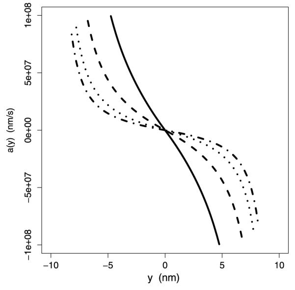
The WLC drift function for four values of L_p—0.8 nm (solid), 2 nm (dashed), 4 nm (dotted), and 6 nm (dash-dot)

The FENE model posits a neck linker that allows the tethered head to diffuse with minimal constraint up to its maximum contour length L_c, where the neck linker is inextensible. The corresponding drift function is

$$a\left(y\right)=-\frac{\kappa (y-y_0)}{\zeta }\text{if}\mid y-y_0\mid <L_c,$$ (36)

where κ is a small spring constant (order of 0.1 pN/nm). Conceptually, this drift increases dramatically as the displacement from y₀ increases to L_c, where it abruptly asymptotes. In practice, the transition rates for the approximating Markov chain are set to zero, thus preventing movement outside the set boundaries. For each neck linker mechanical model, motor velocity, effective diffusion, and run length (the distance the motor moves along the filament during each encounter with the microtubule) were calculated for motors having a range of neck linker extensions, matching the motor constructs studied by Yildiz et al. (2008).

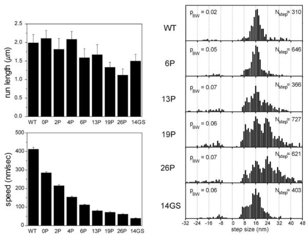
The wild-type Kinesin-1 neck linker is 14 amino acids in length, and Yildiz et al. (2008) introduced variable numbers of proline residues along with two lysines to add positive charge and one glycine to provide flexibility to extend the neck linker. They found that extending the neck linker decreased motor velocity but had only a minimal impact on motor processivity as measured by the run length. These data are reproduced in Fig. 7, along with distributions of measured step sizes, which were measured by tracking quantum dots attached to one of the two heads.

Fig. 7.

Experimental results from Yildiz et al. (2008). At left, run length and speed from single molecule assays of kinesins engineered with extended neck linker domains. At right, step size distributions, measured by monitoring the position of a quantum dot attached to one head domain. With this geometry, a normal 8-nm step taken by the motor corresponds to a 16-nm displacement of the labeled head domain (steps in which the unlabeled head takes a step correspond to zero displacement and are not recorded). 6P to 26P correspond to the number of proline residues inserted into the neck linker domain (in addition to two lysines and one glycine), and 14GS denotes a 14 amino acid insert containing glycine and serine residues. Permission for figure pending from Cell Press (Dec, 2010)

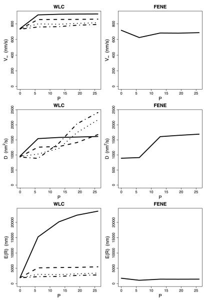
The calculations for the first model incorporated tethered diffusion of the free head but did not explicitly consider tension between the heads, such that when larger steps were taken, the subsequent detachment rate constants were unchanged (see state 1 in Fig. 4). In these “strain-independent” calculations incorporating the WLC, motor velocity increased moderately with increasing neck linker length for all L_p values tested (see Fig. 8). Extending the neck linker had the biggest effect when the WLC was the stiffest (L_p = 0.8 nm) because the forces constraining diffusion of the head were the largest in this case, and extending the neck linker allowed the tethered head to reach the next binding site more rapidly. The motor run length also increased when the neck linker was extended, with L_p = 0.8 nm again showing the strongest dependence on the neck linker length for a similar reason. Faster stepping minimizes the probability that the bound head will detach before the tethered head binds to its next binding site (state 4 in Fig. 4), enhancing processivity. Hence, the strain-independent calculations using the WLC model failed to reproduce the trends seen in the experimental data. These velocity and run length data are qualitatively consistent with our previous calculations using uniform steps (Kutys et al. 2010; Hughes et al. 2011).

Fig. 8.

Comparison of WLC and FENE for the no tension scenario. Each plot shows asymptotic velocity, effective diffusion, or expected run length for various neck linker lengths—WT, 6P, 13P, 19P, and 26P. Each WLC plot shows curves for four values of L_p—0.8 nm (solid), 2 nm (dashed), 4 nm (dotted), and 6 nm (dash-dot). The spring constant for the FENE model was set at κ = 0.1

For calculations incorporating the FENE neck linker model, extending the neck linker had little effect on either run length or velocity (Fig. 8), also in conflict with the experimental results. The reason for this lack of dependence is that, because the diffusional search is only minimally constrained by the neck linker, extending the tether does not substantially reduce the time it takes for the tethered head to bind. The small decrease in run length and velocity for the 6 proline insertion results from the diffusional search space being increased without allowing any more binding sites to be accessed. Increasing the insertion to 13 prolines allows access to the next tubulin binding site, permitting the motor to straddle the adjacent tubulin, resulting in an enhanced velocity and run length. Hence, neither the WLC, nor the FENE using the strain-independent setting were able to faithfully reproduce the experimental data. These results are qualitatively consistent with previous calculations using uniform steps (Kutys et al. 2010; Hughes et al. 2011) and are in conflict with the experimental results from Yildiz et al. (2008).

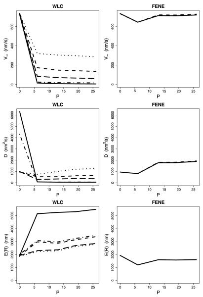
The next calculations, which we term the strain-dependent model, explicitly incorporated inter-head tension. When motors with extended neck linkers took larger steps, the subsequent strain-dependent rate constants (state 1 in Fig. 4) were adjusted accordingly. Hence, this model not only includes variable-length steps, it also incorporates the two gating mechanisms, front-head gating and rear-head gating, thought to underlie kinesin processivity (Block 2007; Rosenfeld et al. 2003; Hancock and Howard 1999). Front head gating, which is implicitly incorporated into all of the models, is achieved by not allowing ATP to bind to the leading head in state 1 until the rear head detaches. Rear-head gating (strain-dependent head detachment) was incorporated into the strain-dependent model by scaling the default rates of k_detach and $k_{\text{attach}}^{\prime }$ by exp(–ζa(8 · S*)d_b/k_BT) as presented in Sect. 4.2. When this strain-dependent detachment was incorporated into the model, the FENE model was not substantially different from the no-tension case. Larger neck linker extensions had a minimal effect on the motor velocity and run length (Fig. 9). This result makes sense because the 0.1 pN/nm stiffness means that the inter-head tension built up when the motor takes a large step has little effect on the resulting strain-dependent rate constants. Hence, in no case was the FENE model able to reproduce the experimental data.

Fig. 9.

Comparison of WLC and FENE for the scenario of strain-dependent detachment. Each WLC plot shows curves for various combinations of d_b and L_p—(2, 2) (solid); (2, 4) (short dash); (2, 6) (dot); (4, 4) (dash-dot); and (4, 6) (long dash). Each FENE plot shows curves for d_b equal to 2 (solid) and 4 (long dash) (with κ = 0.1)

Incorporating strain-dependent detachment kinetics into the WLC model changes the behavior in a number of ways. The first effect of extending the neck linker is to enhance the stepping kinetics by diminishing the restoring force limiting diffusion of the tethered head to its next binding site (state 4 in Fig. 4). Second, with longer neck linkers, the tethered head can also diffuse to binding sites beyond the adjacent tubulin subunit, increasing the step size. On the other hand, extending the neck linker also decreases the strain-dependent detachment kinetics of the trailing head (state 1 in Fig. 4) such that motors with extended neck linkers wait longer in state 1. But larger steps also lead to enhanced inter-head tension, mitigating the effect of neck linker extensions on motor velocity. As seen in Fig. 9, velocity decreased with neck linker extension for all cases, while the run length increased for the stiffest neck linker with the smallest characteristic bond distance (d_b = 2 nm, L_p = 2 nm) and was relatively flat for other parameters tested. Thus, by incorporating strain-dependent detachment kinetics into the variable step model, the qualitative dependence of motor velocity and run length observed experimentally by Yildiz et al. (2008) could be reproduced.

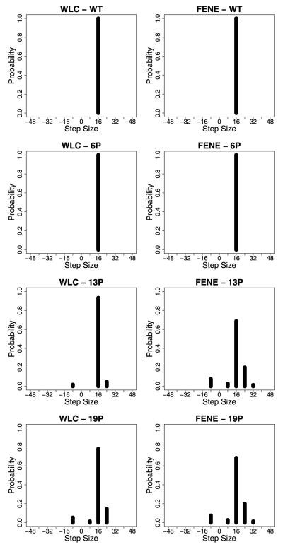
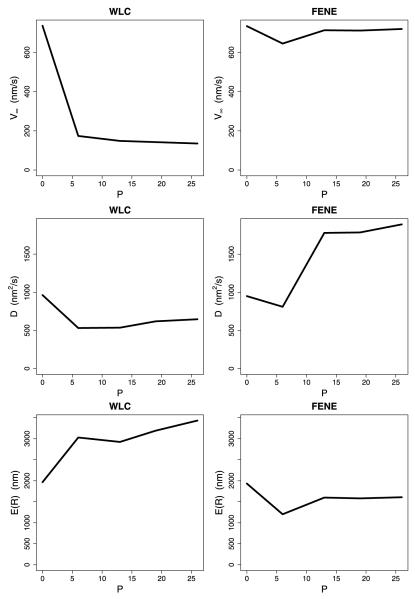
In addition to calculating the velocity and run length results, the model was able to reproduce the experimentally observed distribution of step sizes for neck linker extended kinesins (Yildiz et al. 2008). When one motor domain is labeled, wild-type kinesin is observed to take uniform 16-nm steps, but as the neck linker is extended both larger steps of 24 and 32 nm are seen (corresponding to straddling one or two tubulin binding sites) as well as backward steps (Fig. 7). The step size distributions for the WLC strain-dependent model shown in Fig. 10 qualitatively match the experimental data. Figure 11 shows the dependency of the velocity, effective diffusion, and run length on neck linker extension using the parameters corresponding to Fig. 10. In fact, most of the models tested with different WLC parameters as well as the FENE models reproduced the experimental step size distributions fairly well.

Fig. 10.

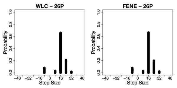
Step-size distributions for the strain-dependent detachment scenario, assuming that only one head has been tagged. For the WLC plots, d_b = 2 and L_p = 4, and for the FENE plots, d_b = 2

Fig. 11.

Plots of V_∞, D, and $\mathbb{E}$R that correspond to the distributions shown in Fig. 10

One interesting point is that extending the neck linker did not substantially change the mean step size because, although longer neck linkers resulted in both larger forward steps, they also resulted in a higher frequency of backward steps (Fig. 12). Instead, the change in velocity results in changes in the cycle duration. The insight highlights one benefit of the method presented in the paper. Decomposing the movement of the motor by time may give additional biological insight; this contrasts the WPE-type methods where the decomposition is in space rather than time (Hackney et al. 2003).

Fig. 12.

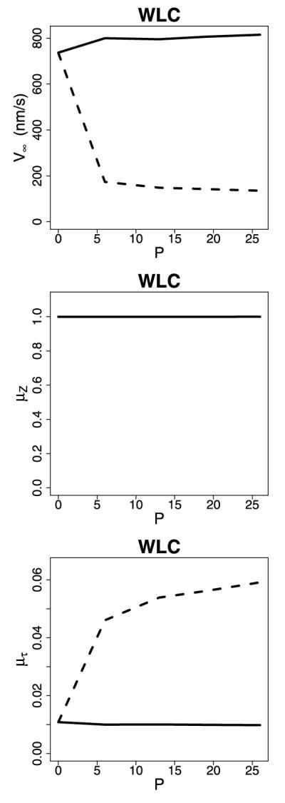
Plots of V_∞, μ_Z, and μ_τ versus neck linker length for the WLC model in the strain-dependent detachment (dashed) and no strain-dependent detachment (solid) scenarios. L_p = 4 for both scenarios, and d_b = 2 for the strain-dependent detachment scenario

6 Conclusions

In this paper, we have presented a model for variable-length stepping based on a previous framework for uniform-length stepping (Kutys et al. 2010; Hughes et al.2011). This formulation is necessary for modeling kinesin with significantly extended neck linker domains and is also applicable to modeling processive myosin and dynein motors that are known to take variable-length steps. In the previous uniform-length stepping framework, the dynamics of each step was independent of the previous step, and the stochastic process describing the position of the motor could be represented by a modification of a renewal-reward process.

The modeling approach described here requires consideration of the initial separation between the heads of the motor at the beginning of each cycle. We showed that this sequence of separation values form a stationary Markov chain and can be included in the calculation of standard experimental quantities, and the process describing the position of the motor is a particular type of semi-Markov process. Moreover, this can be done using relatively efficient matrix calculations instead of time-consuming large-scale stochastic simulations. This greatly facilitates sensitivity analysis, an important feature when there is substantial uncertainty in the physical parameters of the system.

By incorporating the differences in strain for different initial separations of the heads, we showed that a worm-like chain model for the neck linker is consistent with the data presented by Yildiz et al. (2008) and that the inter-head tension is a necessary component in kinesin stepping. This stands in contrast to the earlier modeling results presented by Hughes et al. (2011) and Kutys et al. (2010), which found the finitely extensible neck linker to be more plausible. By using a WLC model for the extensibility of the neck linker and incorporating force-dependent detachment kinetics, the dependence of motor velocity and run length on neck linker extension as well as the distribution of step sizes from Yildiz et al. (2008) were explained.

Appendix A. Pseudocode and Computational Miscellanea

Here we provide pseudocode for the matrix computations and show how to choose the extents of the spatial grid. We use θ to denote the set of input parameters for the chemical model and the approximate diffusion, and so θ includes chemical rates, a spring constant (for the FENE scenario), binding radius, etc. Argument s^max denotes the maximum separation of the heads when both heads are bound.

Algorithm A.1: ComputeVaristep(θ, s^max)

$$\begin{array}{cc}\hfill & \mathbf{for}{s}^{\ast }\leftarrow 1\mathbf{to}{s}^{\max }\hfill \\ \hfill & \mathbf{do}\{\begin{array}{c}\text{Construct}\mathbf{Q}\text{using}\theta \text{and}{s}^{\ast }.\hfill \\ \text{Extract}\mathbf{A}\left(s^{\ast }\right)\text{from}\mathbf{Q}\text{and invert it}.\hfill \\ \text{Extract}\mathbf{B}\left(s^{\ast }\right).\hfill \\ \text{Compute}\mathit{v}=\mathbb{P}(Z\mid S^{\ast }=s^{\ast }).\hfill \\ {\mu }_{Z\mid S^{\ast }}={\mathit{v}}^{\prime }z\hfill \\ {\eta }_{Z\mid S^{\ast }}={\mathit{v}}^{\prime }{z}_2\hfill \\ {\mu }_{\tau \mid S^{\ast }}=-{\mathit{a}}^{\prime }{\left[\mathbf{A}\right(s^{\ast }\left)\right]}^{-1}1\hfill \\ {\eta }_{\tau \mid S^{\ast }}=2{\mathit{a}}^{\prime }{\left[\mathbf{A}\right(s^{\ast }\left)\right]}^{-2}1\hfill \\ {\mu }_{Z\tau \mid S^{\ast }}={\mathit{a}}^{\prime }{\left[\mathbf{A}\right(s^{\ast }\left)\right]}^{-2}\mathbf{B}\left(s^{\ast }\right)z\hfill \\ \text{Compute}\mathit{u}\left(s^{\ast }\right)=\mathbb{P}(S\mid S^{\ast }=s^{\ast }).\hfill \end{array}\phantom{\}}\hfill \end{array}$$

Use the u(s*) to construct the tpm for {S}, P_S|S*.

Perform an eigendecomposition of P’_S|S* and select the principal eigenvector as πS.

${\mu }_{\tau }={\mu }_{\tau \mid S^{\ast }}^{\prime }{\pi }_S$

${\mu }_Z={\mu }_{Z\mid S^{\ast }}^{\prime }{\pi }_S$

${\sigma }_{\tau }^2={\eta }_{\tau \mid S^{\ast }}^{\prime }{\pi }_S-{\mu }_{\tau }^2$

${\sigma }_Z^2={\eta }_{Z\mid S^{\ast }}^{\prime }{\pi }_S-{\mu }_Z^2$

${\sigma }_{Z,\tau }={\mu }_{Z\tau \mid S^{\ast }}^{\prime }{\pi }_S-{\mu }_Z{\mu }_{\tau }$

V_∞ = Lμ_Z/μ_τ

$D=(V_{\infty }^2{\sigma }_{\tau }^2+L^2{\sigma }_Z^2-2L{V}_{\infty }{\sigma }_{Z,\tau })∕\left(2{\mu }_{\tau }\right)$

return V_∞,D

We use a few trial runs of the above algorithm to choose the proper extents of the spatial grid, which are controlled by s^max. For each candidate s^max, we use a sequence of n spatial locations ranging from –(2s^max + 1) · L to (s^max + 1) · L. If the resulting tpm for {S} is stochastic (or at least nearly so), the current value of s^max is sufficiently large given θ. Otherwise, increase the candidate value of s^max and perform another iteration of the algorithm. As s^max increases, so should n. We used s^max = 6 and n = 1,000 to produce the plots in this paper.

Appendix B. Mapping Our Theoretical Variable-Step Results to Experimental Results

Our model keeps track of both heads and accounts for “steps” of zero length, but in experiments, only one head is tagged, and we cannot observe a renewal unless the tagged head changes location. Hence, our theoretical distribution for Z does not match the empirical step-size (henceforth Y ) distribution. In this section, we develop a mapping from πZ to πY so that the results of an in silico experiment can be compared with those of an in vitro experiment.

The mapping uses the joint distribution of S* and S. We can compute the joint pmf as ∏_S*,S = P_S|S* ● πS. This matrix is s^max × s_max. For each pair of starting and ending separations, (s*, s), an experimentalist can see five possible step sizes: 0, ±(s* + s), ±(s* − s). This implies that Y ∈ {0, ±1, … , ±2s^max}.

We need to apportion the s*, s entry of ${\Pi }_{S^{\ast },S,}\mathrm{i}.\mathrm{e}.,p=\mathbb{P}(S^{\ast }=s^{\ast },S=s)$, to the possible values of Y. We do so by handling four cases: RR, RF, FR, and FF, where each pair codes (tagged head, detached head). For example, RR means that the motor’s rear head is tagged and the front head detaches. If we are about to observe the motor, (rear head tagged)/(front head tagged) is a fair coin, and so we assign mass p/2 to each of {RR, RF} and {FR, FF}.

Now, the events RF and FR correspond to Y = 0 because these events are unobservable. Since these events have mass p/2 = (1 – r)p/2 + rp/2, where $r=\mathbb{P}$(rear head detached) = k_detach/(k_detach + $k_{\text{attach}}^{\prime }$), we assign mass p/2 to Y = 0. It is left to spread mass p/2 across the step sizes that correspond to the events RR and FF. For the first event, the possible step sizes are s* + s and s* − s. For the second event, the possible step sizes are –(s* + s) and –(s* − s). It is easy to show that the following mapping Y → Z holds:

$$s^{\ast }+s\to s,$$ (37)

$$s^{\ast }-s\to 0,$$ (38)

$$-(s^{\ast }+s)\to -s^{\ast },$$ (39)

$$-(s^{\ast }-s)\to -(s^{\ast }-s).$$ (40)

This implies the following assignments for the remaining mass:

$$\mathbb{P}(Y=s^{\ast }+s)\leftarrow \mathbb{P}(Y=s^{\ast }+s)+r\frac{\mathbb{P}(Z=s)}{\mathbb{P}(Z=s)+\mathbb{P}(Z=0)}p∕2,$$ (41)

$$\mathbb{P}(Y=s^{\ast }-s)\leftarrow \mathbb{P}(Y=s^{\ast }-s)+r\frac{\mathbb{P}(Z=0)}{\mathbb{P}(Z=s)+\mathbb{P}(Z=0)}p∕2,$$ (42)

$$\begin{array}{cc}\hfill \mathbb{P}(Y=-(s^{\ast }+s\left)\right)\leftarrow & \mathbb{P}(Y=-(s^{\ast }+s\left)\right)\hfill \\ \hfill & +(1-r)\frac{\mathbb{P}(Z=-s^{\ast })}{\mathbb{P}(Z=-s^{\ast })+\mathbb{P}(Z=-(s^{\ast }-s\left)\right)}p∕2,\hfill \end{array}$$ (43)

$$\begin{array}{cc}\hfill \mathbb{P}(Y=-(s^{\ast }-s\left)\right)\leftarrow & \mathbb{P}(Y=-(s^{\ast }-s\left)\right)\hfill \\ \hfill & +(1-r)\frac{\mathbb{P}(Z=-(s^{\ast }-s\left)\right)}{\mathbb{P}(Z=-s^{\ast })+\mathbb{P}(Z=-(s^{\ast }-s\left)\right)}p∕2.\hfill \end{array}$$ (44)

References

- Atzberger P, Peskin C. Bull. Math. Biol. 2006;68(1):131. doi: 10.1007/s11538-005-9003-6. [DOI] [PubMed] [Google Scholar]
- Block S. Biophys. J. 2007;92(9):2986. doi: 10.1529/biophysj.106.100677. [DOI] [PMC free article] [PubMed] [Google Scholar]
- Block SM, Goldstein LS, Schnapp BJ. Nature. 1990;348(6299):348. doi: 10.1038/348348a0. [DOI] [PubMed] [Google Scholar]
- Chen Y, Yan B, Rubin RJ. Biophys. J. 2002;83(5):2360. doi: 10.1016/S0006-3495(02)75250-8. doi:10.1016/S0006-3495(02)75250-8. [DOI] [PMC free article] [PubMed] [Google Scholar]
- Cross R. Trends Biochem. Sci. 2004;29(6):301. doi: 10.1016/j.tibs.2004.04.010. [DOI] [PubMed] [Google Scholar]
- Das RK, Kolomeisky AB. J. Phys. Chem. B. 2008;112(35):11112. doi: 10.1021/jp800982b. doi:10.1021/jp800982b. [DOI] [PubMed] [Google Scholar]
- Fricks J, Wang H, Elston T. J. Theor. Biol. 2006;239(1):33. doi: 10.1016/j.jtbi.2005.07.010. [DOI] [PubMed] [Google Scholar]
- Gilbert SP, Webb MR, Brune M, Johnson KA. Nature. 1995;373(6516):671, 0028–0836. doi: 10.1038/373671a0. Journal Article. [DOI] [PMC free article] [PubMed] [Google Scholar]
- Hackney D, Stock M, Moore J, Patterson R. Biochemistry. 2003;42(41):12011. doi: 10.1021/bi0349118. [DOI] [PubMed] [Google Scholar]
- Hancock W, Howard J. Molecular motors. Wiley-VCH; Weinheim: 2003. Kinesins: processivity and chemomechanical coupling; pp. 243–269. [Google Scholar]
- Hancock W, Howard J. Proc. Natl. Acad. Sci. USA. 1999;96(23):13147. doi: 10.1073/pnas.96.23.13147. [DOI] [PMC free article] [PubMed] [Google Scholar]
- Howard J. Sinauer; Sunderland: 2001. [Google Scholar]
- Hughes J, Hancock WO, Fricks J. J. Theor. Biol. 2011;269(1):181. doi: 10.1016/j.jtbi.2010.10.005. doi:10.1016/j.jtbi.2010.10.005. [DOI] [PubMed] [Google Scholar]
- Julicher F, Ajdari A, Prost J. Rev. Mod. Phys. 1997;69(4):1269. [Google Scholar]
- Kolomeisky AB, Fisher ME. Biophys. J. 2003;84(3):1642. doi: 10.1016/S0006-3495(03)74973-X. http://www.sciencedirect.com/science/article/pii/S000634950374973X. [DOI] [PMC free article] [PubMed] [Google Scholar]
- Kolomeisky A, Fisher M. Ann. Rev. Phys. Chem. 2007 doi: 10.1146/annurev.physchem.58.032806.104532. [DOI] [PubMed] [Google Scholar]
- Kushner H, Dupuis P. Numerical methods for stochastic control problems in continuous time. Springer; Berlin: 2001. [Google Scholar]
- Kutys M, Fricks J, Hancock W. PLoS Comput. Biol. 2010;6(11):7004. doi: 10.1371/journal.pcbi.1000980. [DOI] [PMC free article] [PubMed] [Google Scholar]
- Mallik R, Carter BC, Lex SA, King SJ, Gross SP. Nature. 2004;427(6975):649, 1476–4687. doi: 10.1038/nature02293. Journal Article. [DOI] [PubMed] [Google Scholar]
- Mather W, Fox R. Biophys. J. 2006;91(7):2416. doi: 10.1529/biophysj.106.087049. [DOI] [PMC free article] [PubMed] [Google Scholar]
- Mogilner A, Wang H, Elston T, Oster G. In: Computational cell biology. Fall C, Marland E, Wagner J, Tyson J, editors. Springer; New York: 2002. [Google Scholar]
- Muthukrishnan G, Zhang Y, Shastry S, Hancock W. Curr. Biol. 2009;19(5):442. doi: 10.1016/j.cub.2009.01.058. [DOI] [PMC free article] [PubMed] [Google Scholar]
- Pauling L, Corey R, Branson H. Proc. Natl. Acad. Sci. USA. 1951;37(4):205. doi: 10.1073/pnas.37.4.205. [DOI] [PMC free article] [PubMed] [Google Scholar]
- Rock RS, Rice SE, Wells AL, Purcell TJ, Spudich JA, Sweeney HL. Proc. Natl. Acad. Sci. USA. 2001;98(24):13655, 0027–8424. doi: 10.1073/pnas.191512398. Journal Article. [DOI] [PMC free article] [PubMed] [Google Scholar]
- Rosenfeld S, Fordyce P, Jefferson G, King P, Block S. J. Biol. Chem. 2003;278(20):18550. doi: 10.1074/jbc.M300849200. [DOI] [PMC free article] [PubMed] [Google Scholar]
- Schief W, Howard J. Curr. Opin. Cell Biol. 2001;13(1):19. doi: 10.1016/s0955-0674(00)00169-1. [DOI] [PubMed] [Google Scholar]
- Shaevitz JW, Block SM, Schnitzer MJ. Biophys. J. 2005;89(4):2277. doi: 10.1529/biophysj.105.064295. http://www.sciencedirect.com/science/article/pii/S000634950572871X. [DOI] [PMC free article] [PubMed] [Google Scholar]
- Shastry S, Hancock WO. Curr. Biol. 2010;20(10):939. doi: 10.1016/j.cub.2010.03.065. doi:10.1016/j.cub.2010.03.065. [DOI] [PMC free article] [PubMed] [Google Scholar]
- Vale R, Milligan R. Science. 2000;288(5463):88. doi: 10.1126/science.288.5463.88. [DOI] [PubMed] [Google Scholar]
- Vale RD, Funatsu T, Pierce DW, Romberg L, Harada Y, Yanagida T. Nature. 1996;380(6573):451. doi: 10.1038/380451a0. [DOI] [PMC free article] [PubMed] [Google Scholar]
- Wang H, Qian H. J. Math. Phys. 2007;48(1):013303. [Google Scholar]
- Wang H, Peskin C, Elston T. J. Theor. Biol. 2003;221(4):491. doi: 10.1006/jtbi.2003.3200. [DOI] [PubMed] [Google Scholar]
- Whitt W. Stochastic-process limits: an introduction to stochastic-process limits and their application to queues. Springer; Berlin: 2002. [Google Scholar]
- Xing J, Wang H, Oster G. Biophys. J. 2005;89(3):1551. doi: 10.1529/biophysj.104.055178. [DOI] [PMC free article] [PubMed] [Google Scholar]
- Yildiz A, Tomishige M, Gennerich A, Vale R. Cell. 2008;134:1030. doi: 10.1016/j.cell.2008.07.018. [DOI] [PMC free article] [PubMed] [Google Scholar]
- Yildiz A, Tomishige M, Gennerich A, Vale R. Cell. 2008;134(6):1030. doi: 10.1016/j.cell.2008.07.018. [DOI] [PMC free article] [PubMed] [Google Scholar]