

SUMMARY
The Centers for Disease Control and Prevention defined epilepsy as an emerging public health issue in a recent report and emphasized the importance of epilepsy studies in minorities and people of low socioeconomic status. Previous research has suggested that the incidence rate for epilepsy is positively associated with various measures of social and economic disadvantage. In response, we utilize hierarchical Bayesian models to analyze health disparities in epilepsy and seizure risks among multiple ethnicities in the city of Philadelphia, Pennsylvania. The goals of the analysis are to highlight any overall significant disparities in epilepsy risks between the populations of Caucasians, African Americans, and Hispanics in the study area during the years 2002–2004 and to visualize the spatial pattern of epilepsy risks by ethnicity to indicate where certain ethnic populations were most adversely affected by epilepsy within the study area. Results of the Bayesian model indicate that Hispanics have the highest epilepsy risk overall, followed by African Americans, and then Caucasians. There are significant increases in relative risk for both African Americans and Hispanics when compared with Caucasians, as indicated by the posterior mean estimates of 2.09 with a 95 per cent credible interval of (1.67, 2.62) for African Americans and 2.97 with a 95 per cent credible interval of (2.37, 3.71) for Hispanics. Results also demonstrate that using a Bayesian analysis in combination with geographic information system (GIS) technology can reveal spatial patterns in patient data and highlight areas of disparity in epilepsy risk among subgroups of the population.
Keywords: hierarchical Bayesian regression, health disparities, spatial epidemiology, MCMC, spatial statistics
1. INTRODUCTION
Epilepsy is a neurological disorder marked by recurrent, unprovoked seizures. It has been estimated that at least 2.5 million people are being treated for epilepsy in the United States alone [1] and 150 000 people are newly diagnosed with epilepsy each year [2]. There are a range of etiologies and risk factors for epilepsy, many of which show geographic variation, which in turn lead to spatial variation in epilepsy incidence and prevalence rates [2–4]. Some etiologies include genetic conditions, central nervous system infections, cancer, and cerebrovascular disease. However, the full range of etiologies is not known and predictors of epilepsy outcomes are not well established. In addition, it is difficult to diagnose individual cases of epilepsy [2, 5], and incidence and prevalence estimates are generally thought to be underestimates due to the difficulty in case attainment, as individuals with epilepsy may not seek medical treatment due to lack of education regarding symptoms or stigma [6, 7]. Comorbidity in epilepsy is also a major concern, as epilepsy patients tend to have higher risks for various somatic and psychiatric disorders [8].
Previous research suggests that incidence and prevalence rates for epilepsy are positively associated with various measures of social and economic disadvantage, such as residence overcrowding and unemployment [9–11]. This pattern also appears at the international scale where prevalence and incidence estimates are generally higher in developing countries than in developed countries [2]. The Centers for Disease Control and Prevention and the Epilepsy Foundation defined epilepsy as an emerging public health issue in a recent report ‘Living Well with Epilepsy II’ and emphasized the importance of epilepsy studies focusing on minorities and people of low socioeconomic status [7].
The increasing interest on health disparities in specific outcomes such as epilepsy builds on the broad literature on health disparities. The U.S. federal government, as part of the initiative Healthy People 2010 [12], aims to reduce or eliminate health disparities among subgroups of the population, where disparities may be based on numerous factors, including ethnicity and geographic location. A 2005 report on health disparities from the Agency for Healthcare quality revealed that significant gaps still exist for those who are non-Caucasian for many chronic health conditions [13]. Typically, African Americans and Hispanics, compared with Caucasians, experience higher morbidity and mortality for many diseases as well as shorter lifespans and lower rates of insurance coverage [14]. Minorities receive less continuity of care and utilize hospital clinics and community health centers more than non-minorities [15]. Hispanic adults are substantially less likely than non-Hispanic adults to receive preventive services such as cancer screenings, cholesterol screening and vaccinations [16], and access to care issues play an important role in the relationship between quality of healthcare and the presence of health disparities [17] since insurance status and socioeconomic differences account for a large amount of disparities in health and healthcare among minorities [18].
In response to the need for analyses of epilepsy in minority populations, we utilize hierarchical Bayesian models to analyze health disparities in epilepsy and seizure risk among multiple ethnicities in the city of Philadelphia, Pennsylvania. The goals of the analysis are to highlight any overall significant disparities in epilepsy and seizure risk between the populations of Caucasians, African Americans, and Hispanics in the study area during the years 2002–2004 and to visualize the spatial pattern of epilepsy risk by ethnicity to indicate where certain ethnic populations were most adversely affected by epilepsy within the study area. We set out to analyze ethnic disparities in rates of inpatient and outpatient epilepsy patients from the five hospitals in the Temple University Health System (TUHS) and inpatient epilepsy data from the Pennsylvania Health Care Containment Council (PHC4) system between the years 2002 and 2004 at the ZIP Code level. Some quality issues with data from PHC4 limited our statistical modeling to only the TUHS data, as discussed in detail below.
Race and ethnicity are closely related concepts and the terms ethnicity and race are often used synonymously in practice [19, 20]. However, in the U.S. Census and other survey-based data collection systems race and ethnicity assignments are derived from two different response items. The first, race, refers to the respondent’s self-identification with one or several of a listed set of racial classifications. The second, ethnicity, refers to the respondent’s yes/no response regarding Hispanic origin. As previously reported epilepsy prevalence rates differ between individuals reporting Hispanic origin, and non-Hispanic individuals reporting African-American race and Caucasian race, we concentrate on these three groups. For convenience, we use the term ethnicities to refer to the population groups in the study, even though the classification is based on responses to both the race and ethnicity questions. Ethnicity is a useful concept with which to analyze health within a population, as it helps to differentiate between social and environmental exposures over time that can lead to inequalities in health status [19]. However, there is often heterogeneity within an ethnic group, and research typically underestimates this heterogeneity [20]. The focus on ethnicity in the present study may be helpful in generating testable hypotheses about epilepsy etiology and also for planning and delivering healthcare and public educational efforts [20]. In addition, healthcare managers can benefit from knowing the geographic and demographic distribution of epilepsy patients in the population to better allocate healthcare resources in their area [2].
2. METHODS
2.1. Data
We obtained three years of administrative epilepsy inpatient and outpatient patient contact data from the five hospitals within the TUHS. The data set included 3947 unique inpatients, 5441 unique outpatients, and 7818 unique patients in Philadelphia with variables for demographics, complete address, and five International Classification of Disease-9th Revision (ICD-9) codes. TUHS patients were classified as having epilepsy or seizures using ICD-9 codes 345.xx and 780.3x from five different diagnosis variables, consistent with codes used in other studies to classify persons with epilepsy and seizures [2, 5]. Patients self-reported their ethnicity in a manner similar to other studies [19] thereby reducing potential deficiencies arising from external classification of patient ethnicity [20]. More specifically, patients self-reported race as white, black, Asian, or other, and also self-reported if they were of Hispanic origin. Based on these ethnicity variables, we first classified patients as Hispanic if they were of Hispanic origin and then as Caucasian, African American, or other, if not of Hispanic origin, yielding four mutually exclusive ethnic groups. To map individual epilepsy patient contacts from the TUHS, patient records were address matched, or geocoded, to a street network using GIS software. Individual records for which an automatic match could not be made were located with Internet-based searches [21, 22] for an overall geolocation rate of 96 per cent of all patient records. Records of individual patient visits were combined to create unique patient records and then patients were aggregated by area and ethnicity to derive epilepsy patient counts. We next calculated smoothed, model-based risk estimates by ethnicity at the ZIP Code level under three different modeling scenarios. There was one ZIP Code in the southeast corner of the study area with no inhabitants, and we did not produce estimates for this area.
2.2. Hierarchical Bayesian models
We use hierarchical Poisson Bayesian models to estimate epilepsy rates in small-area units to account for the instability of crude local rate estimates, where a small number of observed cases or a small ethnic population count in an area would result in an unreliable rate with a large variance. The models require as input the crude relative risk of epilepsy (standardized prevalence ratio), which was estimated using the overall rate of epilepsy in the study data.
We compare and contrast three different models defined by different correlation structures induced by three classes of spatial prior distributions. The first hierarchical Bayesian model jointly estimates the smoothed relative risk of epilepsy for the three ethnicities of interest using an intrinsic multivariate conditional autoregressive (CAR) prior, or MCAR, for the area-specific log-relative risks. See [23] for details on the intrinsic CAR model and [24–26] for details on the proper and intrinsic MCAR models. The Bayesian model estimates smoothed rates of epilepsy by borrowing strength for areas with small populations from the neighboring areas to produce more reliable rates. It also includes an age covariate to account for potential differences in population age structure among the areas. Outputs of the model include posterior estimates of overall epilepsy risk by ethnicity, local risk by ethnicity, and the overall correlation between the rates of different ethnicities. The second hierarchical Bayesian model uses a multivariate convolution (MCON) prior [27] to include both structured and unstructured random effects; see [23, 28] for more details of the convolution prior. The third Bayesian model is a shared component model, introduced by Knorr-Held and Best [29], that includes random effects for spatial structure in risk for each ethnicity, as well as a spatially structured random effect that is common to all ethnicities. These types of hierarchical Bayesian models have been used previously to estimate smoothed rates of two diseases simultaneously [29]. In the work in this paper, we use these models to estimate the risk of one adverse health condition in three different ethnic groups. The motivation for using the models in this way is to both utilize risk factors common to multiple ethnicities and quantify disparities in risk among different ethnicities in a unified framework.
More specifically, we begin with the standardized prevalence ratio estimated by Yi/Ei, where Yi is the observed number of epilepsy cases and Ei is the expected number of cases in region i calculated from the overall epilepsy rate in the data and the 2000 U.S. Census population in each region. The crude relative risk, as estimated by the standardized prevalence ratio, is unstable for several areas in the study because of small expected counts or few observed cases. For example, the highest relative risk among the areas for Hispanics is 20, based on observing two cases where less than 0.1 case is expected. The Bayesian models for smoothing the relative risks each build from a Poisson distribution for the observed cases in region i and for ethnicity k such as
| (1) |
i.e. the epilepsy case counts for ethnicity k and area i, Yik, are assumed to follow independent distributions conditional on the unknown mean, μik. The three types of models we consider each specify the log mean of the expected counts in different ways. We continue the specification of the three models in turn, beginning with the MCAR model.
2.3. MCAR model
The unknown log mean of the counts is specified in the MCAR model as
| (2) |
where the ethnicity-specific baseline log-relative risk is αk, the area-specific log-relative risk for each ethnicity is Sik, xi1 is the covariate for per cent population 65 years and older, and β1 is its associated coefficient. It is convenient to think of Sik as the spatial random effect of unobserved risk factors, which may vary by area and ethnicity. Given the structure of the spatial random effects, log-relative risks for an ethnicity are correlated between areas and risks for the three ethnicities are correlated within each area due to unmeasured risk factors, shared at the area level. The relative risk for ethnicity k in area i is
| (3) |
The ethnicity indices are 1 for African American, 2 for Hispanic, and 3 for Caucasian. The intercept term for baseline relative risk for Caucasians, α3, is set to 0, i.e. it is the referent category.
The hierarchical Bayesian model specification is complete with specification of the parameter prior distributions. An MCAR prior is placed on the Sik spatial random effects, S ~ MCAR(ΣS), where the superscript denotes the type of matrix and not a power. The MCAR prior for the vector of size p of spatially dependent random effects in each area i, Si = (Si1, Si2, …, Sip)′, has a multivariate conditional distribution
| (4) |
where S̄i = (S̄i1, S̄i2, …, S̄ip)′, S̄ik = Σj∈κi Sjk/mi, κi is the set of neighboring areas for area i, and mi is the number of neighbors for area i. The diagonal elements of ΣS are the conditional variances of the Sk’s and the off-diagonal elements are the conditional covariances between pairs of Sk’s.
The prior for the age covariate effect is normal, the priors for the ethnicity-specific relative risk intercepts are improper uniform priors, and the prior for the within-area, between-ethnicity 3×3 variance–covariance matrix, ΣS, is vague inverse Wishart with a hyperparameter scale matrix set to Ω = 0.02·Ip×p, where I is the identity matrix, and degrees of freedom v = p, where p = 3 in this case.
Owing to the administrative nature of the TUHS data, it may be beneficial to include a distance-decay effect to reflect different healthcare utilization patterns as one moves away from TUHS hospitals. As such, we include in another MCAR model, MCAR2, a distance effect to capture utilization patterns that are not fully accounted for in the local CAR spatial random effects. The unknown log mean of the counts with the MCAR2 model is now
| (5) |
where xi2 is the Euclidean distance from each ZIP Code centroid to the closest TUHS hospital and the other terms are as defined in the MCAR model. A non-informative normal prior is placed on β2, the distance covariate parameter.
2.4. MCON model
The MCON prior model is similar to the MCAR model, but also includes an unstructured random effect for each area i and ethnicity k to account for non-spatial over-dispersion. The unknown log mean of the counts is specified in the model as
| (6) |
where Uik is the additional unstructured random effect, and the other terms are as previously defined. The total random effect for each area and ethnicity is now a combination of the structured, Sik, and unstructured, Uik, components, where the Ui’s follow independent multivariate normal distributions. The MCON model has additional flexibility over the MCAR model, in that it allows the data to decide how much of the variation in risk is due to over-dispersion and how much is due to spatial structure.
The prior for the unstructured random effects is multivariate normal, Ui ~ Np(0, ΣU), with an inverse Wishart prior on the covariance matrix ΣU. The priors for the other parameters are the same as those in the MCAR model. The choice of hyperparameters for the prior variances for the S and U components is not an obvious one in the convolution model. As Banerjee et al. [26] point out, in the univariate convolution prior model, using the same hyperparameters for the gamma-distributed precision terms for the unstructured and spatially structured random effects can lead to an unfair prior due to the fact that the unstructured effect precision uses the marginal specification and the structured effect precision uses the conditional specification. These authors give a prior adjustment to make the priors comparable in the univariate case, based on the work in [30]. The adjustment involves making the prior standard deviation for the unstructured effects equal to 0.7 times the prior standard deviation of the structured effects, which is the square root of the prior variance multiplied by m̄, the mean number of adjacent neighbors in the study area. We adopt that line of thinking here in the multivariate case and try two different prior specifications for ΣU, one with equal hyperparameters and one that adjusts the unstructured effects variance prior to make the random effects variance priors equal, called the MCON2 model for convenience. In the first case, the hyperparameter scale matrices are set to ΩS = 0.02·Ip×p and ΩU = 0.02·Ip×p, and in the second case they are ΩS = 0.02·Ip×p and ΩU = 0.01·Ip×p.
2.5. Shared component model
In the shared component model, the spatial variation in relative risk is separated into a common component for all ethnicities and an ethnic-specific component. The unknown log means of the counts for each ethnicity are
| (7) |
where the log-relative risk ηik is specified for each ethnicity as
| (8) |
| (9) |
| (10) |
where the shared component ϕi is specified as
| (11) |
which is the combination of a convolution prior with spatial, , and unstructured, , random effects and the age effect. The ψik’s are the ethnic-specific log-relative risk components defined with a convolution prior as
| (12) |
with spatial random effects Sik and unstructured random effects Uik. δ and γ are scaling factors that allow for unequal risk from the shared component among the ethnicities, and the other terms are as previously defined. Knorr-Held and Best [29] use one scaling parameter for modeling the shared component of two diseases, whereas we require two parameters when considering the dependence in three groups. The relative risk ratios on the shared component are
| (13) |
| (14) |
| (15) |
where the subscripts indicate the ethnicities in the ratio.
It is clear that both the shared component and the ethnic-specific components are spatially structured. We follow [27] in using convolution priors for both components. The spatially structured random effects have CAR priors, Sk ~ CAR(λk) and , where λk and τ are the precisions. The unstructured random effects have independent normal priors, Uik ~ N(0, γk) and , where γk and θ are the precisions. As with the MCON model, we use priors with the same hyperparameters for the spatially structured and unstructured random effects variance terms and ‘fair’ priors with an adjustment in the hyperparameters to make the variance priors more equal. The priors for the precisions of the structured and unstructured random effects in the first case are vague gamma, G(0.5, 0.0005). The priors for the precisions, λk and τ, of the structured random effects are G(0.5, 0.0005) and the priors for the precisions, γk and θ, of the unstructured random effects are G(0.5, 0.001) in the second case. We refer to the model in the first case as SHARED and the model in the second case as SHARED2.
The age covariate is included in the shared component as it is not specific to any ethnicity. We do not include separate ethnic-specific log-relative risk terms, as in the MCAR and MCON models, due to identifiability issues. Instead, we marginalize over the ηik’s to obtain the mean posterior total log-relative risk per ethnicity and marginalize over the ψik’s to calculate the mean posterior ethnic-specific log-relative risk. We use an informative normal prior, N(0, 1), for the age effect parameter to overcome poor identifiability of this parameter in this model. In the shared component model, it is also possible to calculate the fraction of the total variation in relative risk for each ethnicity that is explained by the shared component. In general terms, this quantity, Fk, is calculated from the shared component risk variance divided by the sum of the shared component risk variance and the specific component variance.
2.6. Implementation
For all models, the neighborhood adjacency list used in the spatial effect priors is generated in GeoBUGS [27]. We use Markov chain Monte Carlo simulation in WinBUGS software [31] to provide samples of model parameter values from their joint posterior distribution. We use a ‘burn-in’ period of 20 000 iterations and use 180 000 samples from the joint posterior distribution to calculate posterior mean estimates for the model parameters.
3. RESULTS
The ZIP Code-specific crude relative risks are plotted in Figure 1 for Caucasians, African Americans, and Hispanics. A general distance decay appears in the maps, corresponding to usage patterns with individuals living nearby being more likely to seek treatment at the TUHS hospitals. Comparing ethnicities, the relative risks appear highest for Hispanics, next-highest for African Americans, and lowest for Caucasians. The estimated smoothed epilepsy relative risks from the MCAR model for each ethnic group are plotted in Figure 2. The smoothed relative risks are reduced from the high, unstable crude relative risks in Figure 1. However, the order of elevated risk remains the same, where Hispanics appear to have the highest overall risk, followed by African Americans, and then Caucasians. The smoothed relative risks from the MCON model are plotted in Figure 3. The patterns of relative risk by ethnicity are somewhat similar between the MCAR and MCON models; however, the MCON model shrinks the risks more than the MCAR model does and generates risks that are more similar between ethnicities, especially in the north central part of the study area. The smoothed relative risks from the MCON2 model are displayed in Figure 4. It is apparent from the maps in this figure that the MCON2 model shrinks the ethnic-specific relative risks more to the global mean than does the MCON model. Therefore, making the priors for the random effect terms equal appears to have an effect on the estimated relative risks. The smoothed total relative risk for each ethnicity and the shared relative risk component are presented in Figure 5. The ethnic-specific relative risks from the shared component model are more similar to the MCAR estimates than the MCON estimates. One can see that the shared component is influential in the pattern of relative risks for the individual ethnicities. The estimated relative risks for each ethnicity and the shared component from the SHARED2 model are essentially the same as those from the SHARED model and are therefore omitted due to space constraints. The similarity in the values indicates that adjusting the variance priors to be more comparable has little impact on the shared component model in this case.
Figure 1.
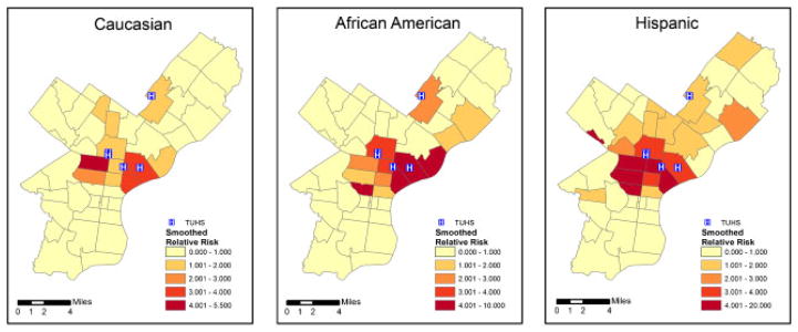
Crude relative risk for epilepsy and seizures by ZIP Code for Caucasians, African Americans, and Hispanics with TUHS hospitals.
Figure 2.
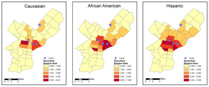
Smoothed relative risk for epilepsy and seizures by ZIP Code for Caucasians, African Americans, and Hispanics from the MCAR model with TUHS hospitals.
Figure 3.
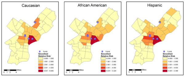
Smoothed relative risk for epilepsy and seizures by ZIP Code for Caucasians, African Americans, and Hispanics from the MCON model with TUHS hospitals.
Figure 4.
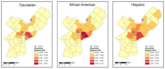
Smoothed relative risk for epilepsy and seizures by ZIP Code for Caucasians, African Americans, and Hispanics from the MCON2 model with TUHS hospitals.
Figure 5.

Total relative risk by ethnicity (top panel) and shared component (bottom panel) for epilepsy and seizures by ZIP Code with TUHS hospitals.
The overall spatial distribution of epilepsy in African Americans appears to be more correlated to the spatial distribution of epilepsy in Hispanics than it does with the spatial distribution of epilepsy in Caucasians. It is also clear that the spatial patterns of epilepsy risk vary by ethnicity and are influenced, but not entirely explained, by the distribution of ethnic populations in Figure 6, which portrays the proportion of the 2000 U.S. Census population that falls into each ethnic group as shaded areas along with the number of epilepsy and seizure patient visits to TUHS hospitals as graduated circles with area proportional to the number of patients.
Figure 6.
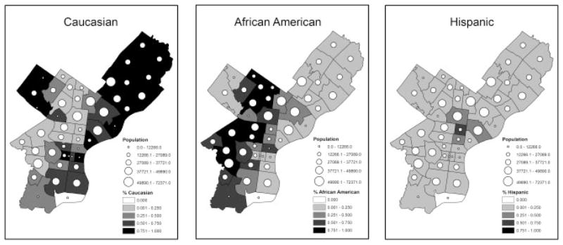
Proportion of the population by ZIP Code that are Caucasians, African Americans, and Hispanics along with the number of TUHS epilepsy and seizure patient visits.
Results of fitting the Bayesian models quantify the visual impressions in the figures. Several parameter estimates from the Bayesian MCAR model are listed in Table I. The indices are as follows: 1 for African American, 2 for Hispanic, and 3 for Caucasian. The relative risks for African American and Hispanic individuals compared with Caucasians are listed in the table. The posterior estimates show that Hispanics have the highest local relative risks, followed by African Americans, and then Caucasians. There are significant increases in relative risk for both African Americans and Hispanics when compared with Caucasians, as indicated by the posterior mean estimates of 2.1 with a 95 per cent credible interval of (1.66, 2.61) for African Americans and 2.97 with a 95 per cent credible interval of (2.36, 3.69) for Hispanics. The posterior correlations between epilepsy risks for different ethnicities indicate that there is a strong shared spatial pattern of risk for epilepsy between the three ethnicities. The correlations are estimated from the covariance matrix of the MCAR prior as . Comparing pairs of ethnicities, the relative risks for African Americans and Hispanics most correspond ( ), followed by Hispanics and Caucasians ( ), and then African Americans and Caucasians ( ).
Table I.
Select parameter posterior estimates from the MCAR model.
| Parameter | Posterior mean | Standard deviation | 2.5 Per cent interval | 97.5 Per cent interval | |
|---|---|---|---|---|---|
| exp(α1) | 2.096 | 0.242 | 1.611 | 2.609 | |
| exp(α2) | 2.967 | 0.341 | 2.357 | 3.690 | |
| β1 | −8.872 | 0.570 | −10.000 | −7.775 | |
|
|
0.930 | 0.038 | 0.838 | 0.983 | |
|
|
0.830 | 0.061 | 0.686 | 0.922 | |
|
|
0.925 | 0.037 | 0.833 | 0.974 |
Parameter estimates from the MCAR2 model are listed in Table II. The estimated ethnic-specific baseline relative risks are similar to those from the MCAR model, as are the posterior correlation estimates. The conclusions from the MCAR model do not change based on these posterior parameter estimates. Including the distance covariate does change the age effect parameter estimate significantly, as it is no longer statistically different from zero. The posterior mean estimate for the distance effect is significantly negative considering the 95 per cent credible interval. There is some positive correlation between percent of the population aged 65 years and older and distance from the nearest TUHS hospital; therefore, this may explain the change in posterior estimate for the age effect. It seems sufficient to include only one of these two effects, and it is more standard to account for potential differences in population age structure.
Table II.
Select parameter posterior estimates from the MCAR2 model.
| Parameter | Posterior mean | Standard deviation | 2.5 Per cent interval | 97.5 Per cent interval | |
|---|---|---|---|---|---|
| exp(α1) | 2.110 | 0.246 | 1.673 | 2.644 | |
| exp(α2) | 2.871 | 0.360 | 2.219 | 3.626 | |
| β1 | −3.197 | 2.689 | −8.313 | 2.465 | |
| β2 | −0.234 | 0.109 | −0.461 | −0.027 | |
|
|
0.905 | 0.049 | 0.783 | 0.974 | |
|
|
0.801 | 0.073 | 0.630 | 0.911 | |
|
|
0.895 | 0.050 | 0.770 | 0.964 |
Some results of fitting the MCON model are listed in Table III. The posterior mean estimates for the ethnic-specific baseline relative risks are similar to the ones from the MCAR model, as one would expect. The age effect posterior mean estimate is also very similar to that from the MCAR model. The correlations of the spatial random effects are again high, although the order of the correlations is different, where the correlation between Hispanics and Caucasians is highest, followed by that for Hispanics and African Americans and then Caucasians and African Americans. The correlations of the unstructured random effects, denoted by the superscript U, are more moderate than with the spatial random effects, and the order of correlations from highest to lowest is the same as that for the spatial random effects in the MCAR model, where Hispanics and African Americans are most correlated ( ) and Caucasians and African Americans are least correlated ( ). The credible intervals are relatively wide for both structured and unstructured effects, but particularly for the unstructured effects, and the structured effect intervals are noticeably wider than in the MCAR model. The total correlations, denoted by the superscript ‘T’, are similar to the correlations of the spatial random effects in the MCAR model, except that the correlation in risk between Hispanics and Caucasians is higher than the correlation between African Americans and Hispanics in the MCON model.
Table III.
Select parameter posterior estimates from the MCON model.
| Parameter | Posterior mean | Standard deviation | 2.5 Per cent interval | 97.5 Per cent interval | |
|---|---|---|---|---|---|
| exp(α1) | 2.020 | 0.288 | 1.355 | 2.567 | |
| exp(α2) | 2.945 | 0.377 | 2.199 | 3.691 | |
| β1 | −8.707 | 1.374 | −10.810 | −4.526 | |
|
|
0.914 | 0.142 | 0.478 | 0.999 | |
|
|
0.908 | 0.151 | 0.454 | 0.999 | |
|
|
0.969 | 0.052 | 0.836 | 0.999 | |
|
|
0.773 | 0.385 | −0.600 | 0.995 | |
|
|
0.485 | 0.655 | −0.953 | 0.995 | |
|
|
0.680 | 0.513 | −0.795 | 0.996 | |
|
|
0.912 | 0.073 | 0.713 | 0.985 | |
|
|
0.870 | 0.096 | 0.608 | 0.969 | |
|
|
0.935 | 0.044 | 0.824 | 0.986 |
The posterior estimates for the MCON2 model are listed in Table IV. The parameter posterior estimates are similar to those from the MCON model, except that the unstructured random effects are overall larger in the MCON2 model. The order of the total correlations is the same in the MCON and MCON2 models. The credible intervals for the unstructured random effects are again large. Separating the variation into structured and unstructured components within the MCON prior leads to wider credible intervals for the total correlations than for the spatial component correlations in the MCAR model, due to the decreased precision in the added unstructured effects.
Table IV.
Select parameter posterior estimates from the MCON2 model.
| Parameter | Posterior mean | Standard deviation | 2.5 Per cent interval | 97.5 Per cent interval | |
|---|---|---|---|---|---|
| exp(α1) | 2.083 | 0.258 | 1.594 | 2.609 | |
| exp(α2) | 3.005 | 0.348 | 2.352 | 3.720 | |
| β1 | −8.898 | 1.069 | −11.240 | −6.753 | |
|
|
0.856 | 0.207 | 0.244 | 0.998 | |
|
|
0.863 | 0.190 | 0.345 | 0.999 | |
|
|
0.958 | 0.072 | 0.774 | 0.998 | |
|
|
0.864 | 0.330 | −0.593 | 0.943 | |
|
|
0.706 | 0.517 | −0.949 | 0.998 | |
|
|
0.842 | 0.379 | −0.691 | 0.998 | |
|
|
0.885 | 0.080 | 0.680 | 0.981 | |
|
|
0.834 | 0.109 | 0.559 | 0.962 | |
|
|
0.920 | 0.050 | 0.789 | 0.980 |
Posterior mean estimates and 95 per cent credible intervals for some parameters from the shared component model are listed in Table V. The total relative risk for African Americans and Hispanics is similar, whereas that for Hispanics is slightly higher. Relative risk for both of these ethnicities is higher than for Caucasians. The specific relative risks are highest for Hispanics and lowest for Caucasians, although there are no significant differences among ethnicities in the specific relative risks. The age effect parameter is not significantly different from zero in the shared component model. The relative risk ratios indicate that the risk on the shared component is higher for Caucasians than for African Americans and Hispanics, and that it is higher for African Americans than for Hispanics, although not significantly so. The posterior mean estimates for the fraction of total variation in relative risks for each ethnicity indicate that for African Americans about 96 per cent of the total between-area variation in risk is captured by the shared component, whereas for Hispanics it is about 88 per cent and for Caucasians it is approximately 78 per cent. There are, however, no significant differences in the shared component fractions among different ethnicities. The posterior estimates from the SHARED2 model are essentially the same as those from the SHARED model and are omitted due to space constraints.
Table V.
Select parameter posterior estimates from the shared component model, SHARED.
| Parameter | Posterior mean | Standard deviation | 2.5 Per cent interval | 97.5 Per cent interval |
|---|---|---|---|---|
| exp(η1) | 1.220 | 0.060 | 1.126 | 1.352 |
| exp(η2) | 1.296 | 0.075 | 1.162 | 1.452 |
| exp(η3) | 0.767 | 0.048 | 0.681 | 0.867 |
| exp(ψ1) | 1.023 | 0.063 | 0.940 | 1.184 |
| exp(ψ2) | 1.178 | 0.129 | 0.997 | 1.442 |
| exp(ψ3) | 1.002 | 0.279 | 0.682 | 1.651 |
| β1 | 0.429 | 1.504 | −2.320 | 3.560 |
| δ | 1.212 | 0.082 | 1.064 | 1.387 |
| γ | 1.714 | 0.311 | 1.227 | 2.470 |
| RR1,2 | 1.167 | 0.171 | 0.885 | 1.573 |
| RR1,3 | 0.692 | 0.090 | 0.520 | 0.881 |
| RR2,3 | 0.602 | 0.099 | 0.407 | 0.810 |
| F1 | 0.959 | 0.058 | 0.807 | 1.000 |
| F2 | 0.877 | 0.084 | 0.682 | 0.999 |
| F3 | 0.783 | 0.058 | 0.640 | 0.868 |
The fits of the models, while considering model complexity, are compared using the deviance information criterion (DIC) [31, 32] values that are listed in Table VI. The value D̄ is the posterior mean of the deviance, D̂ is the point estimate of the deviance, pD is the effective number of parameters and is equal to D̄ − D̂, and DIC = D̄ + pD = D̂ +2·pD. The MCON model generates a substantially lower DIC value than does the MCAR model, which has a lower DIC than the MCAR2 model. The additional unstructured effect component of the MCON model produces a gain in predictive power. The additional distance covariate in the MCAR2 model does not add substantial value, given its association with the age covariate. There is only a small difference in DIC between the MCON and MCON2 models. The shared component model produces a slightly lower DIC than does the MCON model. The DIC’s for the SHARED and SHARED2 models are approximately equal.
Table VI.
DIC values for the Bayesian models.
| Model | DIC | D̄ | D̂ | pD |
|---|---|---|---|---|
| MCAR | 887.80 | 765.48 | 643.16 | 122.32 |
| MCAR2 | 904.88 | 774.22 | 643.57 | 130.65 |
| MCON | 823.14 | 730.93 | 638.73 | 92.21 |
| MCON2 | 825.70 | 730.71 | 635.71 | 95.00 |
| SHARED | 817.80 | 717.56 | 617.33 | 100.23 |
| SHARED2 | 817.48 | 718.63 | 619.79 | 98.85 |
4. DISCUSSION
The results of the three types of hierarchical Bayesian models suggest that the shared component and MCON prior models fit the TUHS data substantially better than the MCAR model, with the shared component model having a slight edge in performance over the MCON prior model. The improvement in fit of the MCON prior model over the MCAR model is in line with the recommendation of Besag et al. [23] to favor the inclusion of the unstructured random effects in the convolution prior model. The choice between the shared component and MCON prior models is less clear, given the relatively small differences in DIC values. The choice between the two is more related to the different structure of the models and the difference in output. For modeling health disparities, the shared component model has an advantage over the MCON prior model due to the ability to map its posterior mean estimate of the shared component θi. Comparing the estimated shared component by area with the posterior ethnic-specific relative risk estimates, as in Figure 5, shows the areas where risks exceed the shared risk for each ethnic group. Decomposing the shared risk visually is more difficult in the MCON relative risks maps in Figures 3 and 4, as any shared background is split across the different ethnic-specific sets of parameters. Although the posterior correlations between epilepsy and seizure risk among pairs of ethnic groups are available from the MCAR and MCON models, the shared risk of epilepsy and seizures among all ethnicities is a feature specifically included in the shared component model specification. In addition, the decrease in DIC with the shared component, compared with the MCON model, while modest, is not unexpected, given that the shared component model essentially adds an area-specific convolution prior for the shared component to the area and ethnic-specific convolution prior of the MCON model.
Another assessment of interest in the analysis was the use of comparable, or fair, priors versus priors with equal hyperparameters for the unstructured and structured model effects. The results of using comparable priors for the spatially structured and unstructured random effects varied depending on the type of model. In the MCON prior model, using comparable priors resulted in more shrinkage in the estimated relative risks to the overall, or global, relative risk with an increase in the correlations of the unstructured effects among the three ethnicities. This is somewhat in contrast to the conclusion by Lindley [33], also noted in [31], that the choice of the prior scale matrix for an inverse Wishart covariance matrix has little impact on its posterior estimate, although the setting and model structure are different here. In contrast, the comparable priors for the structured and unstructured effects in the shared component model had little impact on any of the posterior estimates when compared with the shared component model with the same prior hyperparameters for the structured and unstructured effects.
In analyzing the epilepsy data in this paper, we encountered several difficulties in dealing with administrative data, particularly in merging spatially misaligned data from multiple sources. In addition to the TUHS data, we also obtained inpatient epilepsy data from PHC4, with only ZIP Code available for a patient residence. PHC4 collects data from all general acute-care, psychiatric, rehabilitation, and long-term Pennsylvania hospitals. The data set included 5247 unique inpatients with ZIP Codes in Philadelphia. It contained a larger geographic area than Philadelphia, in which 37 per cent of the patients had no valid ZIP Code listed, but instead were listed as ‘private’. These are thought to be primarily psychiatric or HIV patients. There were some differences in the percent missing ZIP Code by ethnicity. The TUHS database is administrative in nature, whereas the PHC4 database is an aggregation of multiple reporting sources and therefore has the potential for more complete and larger coverage. However, the large percent of missing locational information in the PHC4 data was a difficulty in attempting to synthesize the two epilepsy and seizure data sets, particularly in a spatial analysis. In addition, the PHC4 data contained only patients with a primary diagnosis of seizures or epilepsy, whereas the TUHS data contained five codes for diagnosis of epilepsy or seizures. To maximize the use of both the inpatient and outpatient data from TUHS and to avoid the potential bias of missing data, we elected not to use the PHC4 data.
Another difficulty in working with administrative data is in distinguishing between disease incidence and prevalence. The TUHS data set did not include indicators for patient history of epilepsy or seizures; therefore, it was not possible to estimate incidence rates. Another facet of working with hospital system administrative data is a potential distance-decay effect in observed rates of hospital visits. For example, we expected a significant negative distance-decay effect, given the increased opportunity to visit hospitals of another hospital system, as distance from residence to TUHS hospitals increases. There was a significant distance-decay effect in the MCAR model with the TUHS data, although, curiously, adding the significant distance covariate parameter did not decrease the DIC.
GISs are frequently utilized in public health research for exploring spatial relationships in disease and disparities in access to healthcare services. In addition, Bayesian statistical modeling has proven to be useful in displaying trends and explaining spatial variation in disease rates. Bayesian hierarchical models with MCAR priors, MCON priors, and shared components have previously been beneficial in estimating smoothed rates for multiple diseases simultaneously. Our experience in analyzing epilepsy data from the TUHS demonstrates that using these Bayesian hierarchical models in combination with GIS technology can reveal spatial patterns in patient data and highlight areas of disparity in risk for one disease among several subgroups of the population, in this case different ethnic groups. Furthermore, maps of posterior relative risk estimates illustrate that these disparities vary within the study area in geographically distinctive ways. These patterns can be examined in various ways to improve outreach efforts and patient education programs, as well as for identifying community resources where such programs could be based. Future work will produce subgroup-specific risk estimates at the census tract, neighborhood, and grid level for an examination of scale effects.
Acknowledgments
We would like to thank Dr Mercedes Jacobson, Director of the Temple University Comprehensive Epilepsy Center, for her support in the acquisition of the patient data utilized in this research.
References
- 1.Begley CE, Famulari M, Annegers JF, Lairson DR, Reynolds TF, Coan S, Dubinsky S, Newmark ME, Leibson C, So EL, Rocca WA. The cost of epilepsy in the United States: an estimate from population-based clinical and survey data. Epilepsia. 2000;41:342–351. doi: 10.1111/j.1528-1157.2000.tb00166.x. [DOI] [PubMed] [Google Scholar]
- 2.Holden EW, Nguyen HT, Grossman E, Robinson S, Nelson LS, Gunter MJ, Worley AV, Thurman DJ. Estimating prevalence, incidence, and disease-related mortality for patients with epilepsy in managed care organizations. Epilepsia. 2005;46:311–319. doi: 10.1111/j.0013-9580.2005.30604.x. [DOI] [PubMed] [Google Scholar]
- 3.Sander JW. The epidemiology of epilepsy revisited. Current Opinion in Neurology. 2003;16:165–170. doi: 10.1097/01.wco.0000063766.15877.8e. [DOI] [PubMed] [Google Scholar]
- 4.Kotsopoulos IA, van Merode T, Kessels FG, de Krom MC, Knottnerus JA. A systematic review and meta-analysis of incidence studies of epilepsy and unprovoked seizures. Epilepsia. 2002;43:1402–1409. doi: 10.1046/j.1528-1157.2002.t01-1-26901.x. [DOI] [PubMed] [Google Scholar]
- 5.Holden EW, Grossman E, Nguyen HT, Gunter MJ, Grebosky B, Worley AV, Nelson LS, Robinson S, Thurman DJ. Developing a computer algorithm to identify epilepsy cases in managed care organizations. Disease Management. 2005;1:1–14. doi: 10.1089/dis.2005.8.1. [DOI] [PubMed] [Google Scholar]
- 6.Dalrymple J, Appleby J. Cross sectional study of reporting of epileptic seizures to general practitioners. British Medical Journal. 2000;320:94–97. doi: 10.1136/bmj.320.7227.94. [DOI] [PMC free article] [PubMed] [Google Scholar]
- 7.Shafer PO, Barkley GL, Carr D. Living Well with Epilepsy 2: Report of the 2003 National Conference on Public Health and Epilepsy; Baltimore, MD: Epilepsy Foundation; 2004. [Google Scholar]
- 8.Gaitatzis A, Carroll K, Majeed A, Sander JW. The epidemiology of the comorbidity of epilepsy in the general population. Epilepsia. 2004;45:1613–1622. doi: 10.1111/j.0013-9580.2004.17504.x. [DOI] [PubMed] [Google Scholar]
- 9.Hesdorffer DC, Tian H, Anand K, Hauser WA, Ludvigsson P, Olafsson E. Socioeconomic status is a risk factor for epilepsy in Icelandic adults but not in children. Epilepsia. 2005;46:1297–1303. doi: 10.1111/j.1528-1167.2005.10705.x. [DOI] [PubMed] [Google Scholar]
- 10.Morgan CLI, Ahmed Z, Kerr MP. Social deprivation and prevalence of epilepsy and associated health usage. Journal of Neurology, Neurosurgery, and Psychiatry. 2000;69:13–17. doi: 10.1136/jnnp.69.1.13. [DOI] [PMC free article] [PubMed] [Google Scholar]
- 11.Heaney DC, MacDonald BK, Everitt A, Stevenson S, Leonardi GS, Wilkinson P, Sander JW. Socioeconomic variation in incidence of epilepsy: prospective community based study in south east England. British Medical Journal. 2002;325:1013–1016. doi: 10.1136/bmj.325.7371.1013. [DOI] [PMC free article] [PubMed] [Google Scholar]
- 12.U.S. Department of Health and Human Services. Healthy People 2010: Understanding and Improving Health. 2. U.S. Government Printing Office; Washington, DC: 2000. [Google Scholar]
- 13.McNeill D, Moy E, Clancy CM. The agency for healthcare research and quality’s national healthcare quality and disparities reports: action agendas for the nation. American Journal of Medical Quality. 2006;21:206–209. doi: 10.1177/1062860606288003. [DOI] [PubMed] [Google Scholar]
- 14.Kaplan SA, Calman NS, Golub M, Davis JH, Ruddock C, Billings J. Racial and ethnic disparities in health: a view from the South Bronx. Journal of Health Care for the Poor and Underserved. 2006;17:116–127. doi: 10.1353/hpu.2006.0026. [DOI] [PubMed] [Google Scholar]
- 15.Doescher MP, Saver BG, Fiscella K, Franks P. Racial/ethnic inequities in continuity and site of care: location, location, location. Health Services Research. 2001;36(6 Pt 2):78–89. [PMC free article] [PubMed] [Google Scholar]
- 16.Centers for Disease Control and Prevention. Access to health-care and preventive services among Hispanics and non-Hispanics—United States, 2001–2002. Morbidity and Mortality Weekly Report. 2004;53:937–941. [PubMed] [Google Scholar]
- 17.Freeman G, Lethbridge-Cejku M. Access to health care among Hispanic or Latino women: United States, 2000–2002. Advance Data. 2006;368:1–25. [PubMed] [Google Scholar]
- 18.Kirby JB, Taliaferro G, Zuvekas SH. Explaining racial and ethnic disparities in health care. Medical Care. 2006;44(5 Suppl):I64–I72. doi: 10.1097/01.mlr.0000208195.83749.c3. [DOI] [PubMed] [Google Scholar]
- 19.Bhopal R. Race and ethnicity: responsible use from epidemiological and public health perspectives. Journal of Law, Medicine and Ethics. 2006;34:500–507. doi: 10.1111/j.1748-720x.2006.00062.x. [DOI] [PubMed] [Google Scholar]
- 20.Fustinoni O, Biller J. Ethnicity and stroke: beware of the fallacies. Stroke. 2000;31:1013–1015. doi: 10.1161/01.str.31.5.1013. [DOI] [PubMed] [Google Scholar]
- 21. [Accessed on 26 May 2006];Google Maps. Available at: http://maps.google.com/
- 22.Microsoft Corporation. [Accessed on 26 May 2006];Terra Server USA. Available at: http://terraserver.microsoft.com.
- 23.Besag J, York J, Mollie A. Bayesian image restoration, with two applications in spatial statistics (with discussion) Annals of the Institute of Statistical Mathematics. 1991;43:1–59. [Google Scholar]
- 24.Mardia KV. Multi-dimensional multivariate Gaussian Markov random fields with application to image processing. Journal of Multivariate Analysis. 1988;24:265–284. [Google Scholar]
- 25.Gelfand A, Vounatsou P. Proper multivariate conditional autoregressive models for spatial data analysis. Biostatistics. 2003;4:11–25. doi: 10.1093/biostatistics/4.1.11. [DOI] [PubMed] [Google Scholar]
- 26.Banerjee S, Carlin B, Gelfand A. Hierarchical Modeling and Analysis for Spatial Data. Chapman & Hall/CRC; Boca Raton, FL: 2004. [Google Scholar]
- 27.Thomas A, Best N, Lunn D, Arnold R, Spiegelhalter D. GeoBUGS User Manual, Version 1.2. MRC Biostatistics Unit; Cambridge: 2004. [Google Scholar]
- 28.Mollie A. Bayesian mapping of disease. In: Gilks WR, Richardson S, Spiegelhalter DJ, editors. Markov Chain Monte Carlo in Practice. Chapman & Hall; New York: 1996. pp. 359–379. [Google Scholar]
- 29.Knorr-Held L, Best NG. A shared component model for joint and selective clustering of two diseases. Journal of the Royal Statistical Society, Series A. 2001;164:73–85. [Google Scholar]
- 30.Bernardinelli L, Clayton D, Montomoli C. Bayesian estimates of disease maps: how important are priors? Statistics in Medicine. 1995;16:2411–2431. doi: 10.1002/sim.4780142111. [DOI] [PubMed] [Google Scholar]
- 31.Spiegelhalter DJ, Thomas A, Best NG, Lunn D. WinBUGS User Manual, Version 1.4. MRC Biostatistics Unit; Cambridge: 2003. [Google Scholar]
- 32.Spiegelhalter DJ, Best NG, Carlin BP, van der Linde A. Bayesian measures of model complexity and fit (with discussion) Journal of the Royal Statistical Society, Series B. 2002;64:583–640. [Google Scholar]
- 33.Lindley DV. Foundation of Statistical Inference. Holt, Rinehart and Winston; Toronto: 1970. The estimation of many parameters; pp. 357–371. [Google Scholar]