An Improved Method for the Estimation and Visualization of Velocity Fields from Gastric High-Resolution Electrical Mapping

Abstract

High-resolution (HR) electrical mapping is an important clinical research tool for understanding normal and abnormal gastric electrophysiology. Analyzing velocities of gastric electrical activity in a reliable and accurate manner can provide additional valuable information for quantitatively and qualitatively comparing features across and within subjects, particularly during gastric dysrhythmias. In this study we compared three methods of estimating velocities from HR recordings to determine which method was the most reliable for use with gastric HR electrical mapping. The three methods were i) Simple finite difference ii) Smoothed finite difference and a iii) Polynomial based method. With synthetic data, the accuracy of the simple finite difference method resulted in velocity errors almost twice that of the smoothed finite difference and the polynomial based method, in the presence of activation time error up to 0.5s. With three synthetic cases under various noise types and levels, the smoothed finite difference resulted in average speed error of 3.2% and an average angle error of 2.0° and the polynomial based method had an average speed error of 3.3% and an average angle error of 1.7°. With experimental gastric slow wave recordings performed in pigs, the three methods estimated similar velocities (6.3-7.3 mm/s), but the smoothed finite difference method had a lower standard deviation in its velocity estimate than the simple finite difference and the polynomial based method, leading it to be the method of choice for velocity estimation in gastric slow wave propagation. An improved method for visualizing velocity fields is also presented.

I. Introduction

A rhythmic electrical activity known as slow waves coordinate the motility of the stomach. Slow waves are initiated and propagated by a specialized network of cells termed the ‘interstitial cells of Cajal’ (ICC), which are located in and between the muscular layers of the stomach wall [1]. In the normal human stomach, slow waves propagate from a pacemaker region near the greater curvature of the upper body (corpus) toward the pylorus at a frequency of around three cycles per minute [2]. Dysrhythmic slow wave activity has been associated with several significant motility disorders, including gastroparesis and functional dyspepsia, but abnormal propagation patterns and signal characteristics in humans remain poorly understood [3], [4], [5].

Traditionally sparse serosal electrical mapping or cutaneous electrogastrogram (EGG) have been performed to record and analyze gastric slow wave activity. Due to the sparseness of the electrode configurations or far-field recordings in EGG, propagation patterns and velocities could not be determined accurately [6], [3]. In HR mapping dense arrays of many electrodes are used to track slow wave propagation sequences in spatiotemporal detail [7]. It has recently been shown that gastric serosal HR mapping is a vital technique for evaluating slow wave activity in rhythmic and dysrhythmic states [2], [8], [9]. A major advantage of HR mapping over alternative techniques is the ability to accurately quantify spatial slow wave propagation patterns, providing detailed insights into the initiation, movement and interaction of normal and abnormal wavefronts [8], [9].

Accurate determination of slow wave propagation velocities has become a central focus of gastric HR mapping analysis because substantial changes in velocity have been associated with gastric dysrhythmias indicating abnormal circumferentially propagating wavefronts [10]. Identifying velocity features may therefore allow a better understanding of dysrhythmic slow wave propagation and contribute to an improved foundation for clinically diagnosing gastric dysrhythmias using HR mapping. A reliable and accurate velocity estimation method is therefore required.

In the field of cardiac electrophysiology a number of studies have quantitatively validated different methods of velocity estimation and have guided appropriate usage [11], [12]. Some of the commonly used velocity estimation methods include the use of finite difference, polynomial fitting, and wavelets [11], [12], [13]. However no such validation studies have been conducted for gastric slow wave recordings. Cardiac methods cannot be directly used because of the different signal characteristics of the slow wave events and their propagations patterns during both normal and abnormal activation [14], [15]. As the use of HR gastrointestinal (GI) recording becomes more widespread, there is a pressing need to develop, validate and standardize methods to reliably and efficiently estimate and visualize velocities of slow wave propagations. This would also allow for a fair comparison of velocity outcomes between patient and studies.

In this study we compare three different velocity estimation methods, (i) Finite difference (FD) (ii) Smoothed finite difference (FDSM) and (iii) Polynomial based method (POLY4×4), for gastric HR mapping. These three possible approaches were validated using simulated and experimental data, and outcomes were quantitatively and qualitatively compared to identify the most suitable method for velocity analysis. Improved visualisation methods for velocity fields are also presented.

II. Materials and Methods

A. Experimental Setup

HR gastric mapping was performed on cross-breed weaner pigs following ethical approval from the University of Auckland Animal Ethics Committee. The data was recorded using an ActiveTwo Biosemi System, with 160-256 simultaneous unipolar recordings taken using flexible printed circuit board (PCB) arrays (at 4 mm inter-electrode spacing in a regular grid). The reference (common mode sense) electrode was placed in the lower abdomen in the body, and the right-leg drive electrode was placed on the right hind leg of the body. The electrode array was constructed using multiple flexible PCBs (each 2×16 electrodes - Fig. 1a), which were tessellated together to form a regular recording array, and placed on the serosal surface of the stomach (Fig. 1b). Our methods of anaesthesia, surgery, physiological monitoring and euthanasia have previously been described [16], [9].

Fig. 1.

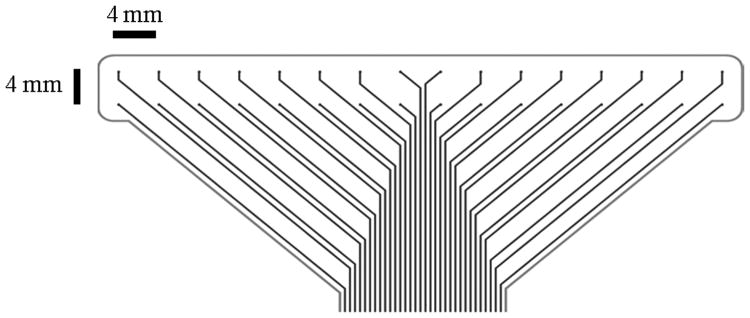
(a) Flexible printed circuit board (PCB) electrode array with an inter-electrode distance spacing of 4mm. (b) Example placement of flexible recording array tessellated and placed on the serosal surface on the antral part of a stomach.

The data was recorded using a sampling frequency of 512 Hz for periods of five to ten minutes. The recorded data was analyzed using Matlab (version 2010a), where the data was first downsampled to 30 Hz, after which a moving median and a Savitzky Golay filter were applied to remove noise from the signals [17]. Then the slow wave activation times were automatically detected using a variable threshold method [15], and clustered into respective propagating waves using a region growing method utilizing a polynomial based surface estimate as a stabilization step [14].

B. Analytic Test Cases

Three synthetic test cases with known velocities were created to test the effectiveness and sensitivity of the velocity estimation methods. The electrode configurations for the test cases were the same as experimental recordings. The first time map follows the form,

$$T(x,y)=ax+by$$ (1)

where T(x, y) represents the time in a 2D activation time map at coordinate locations x and y, while a and b are the coefficients in the equation $(a=b=0.14\overline{14})$. The second and third synthetic time maps were created from an elliptical wave of the form,

$$T(x,y)=K\mathit{sin}(-k_r\sqrt{a{(x-x_0)}^2+b{(y-y_0)}^2})$$ (2)

and approximated with known anisotropic propagation of gastric slow waves [6]. The second synthetic time map was a single source propagation with coefficients K = −30, k_r = −0.25, a = 0.02, b = 0.02 and x₀ = y₀ = 10. The third synthetic time map represented two clashing wavefronts, where the coefficients were K = −30, k_r = −0.25, a = 0.02, b = 0.02, and x₀ = y₀ = 0 for the one of the source and x₀ = y₀ = 60 for the other source.

The first synthetic time map mimics orderly antegrade or retrograde slow wave propagation (Fig. 2a) [2], [9]. The second synthetic time map was an elliptical wave with propagation emerging from the bottom left of the electrode array (Fig. 2b), and mimics ectopic focal activities [8], [9]. The third synthetic time map has two elliptical waves propagating from opposing edges of the electrode array to clash in the center of the array (Fig. 2c), and mimics interacting dysrhythmic activities and gastric pacing [2], [9]. These synthetic time maps were perturbed with random noise (described in III-B) to simulate experimental recordings.

Fig. 2.

(a) Propagation of a linear plane wave (b) Elliptical wave with activity propagating from the center of the electrode array, mimicking ectopic focal slow wave activities. (c) Elliptical wave with activity propagating from the opposing edges of the array to clash in the center, mimicking dysrhythmic slow wave propagation or propagation during gastric pacing.

III. Velocity Estimation Methods

Velocity mapping has been used extensively in cardiac electrophysiology and the methods trialled and validated herein were adapted and developed from a range of previously established techniques. Three methods of velocity estimation are described and compared here with two of the methods in current use in the GI field, and a third new method being introduced. The advantages and disadvantages of the methods are compared and discussed in further detail.

In simple terms, velocity describes the speed and direction of a moving object, which in this context is the slow wave propagation. This is computed by taking the gradient of the time at defined distances. In a two dimensional (2D) case, velocity is computed as follows [11],

$$\left[\begin{array}{c}{V}_x\\ V_y\end{array}\right]=\left[\begin{array}{c}\frac{T_x}{T_x^2+T_y^2}\\ \frac{T_x}{T_x^2+T_y^2}\end{array}\right]$$ (3)

where T_x = ∂T/∂x and T_y = ∂T/∂y are the gradients of the time map with respect to the x and y directions of the recording array.

The simplest approach to estimate velocity on a 2D surface is to take a finite difference (one sided difference for the edges and central difference for the internal points) of the time array. This approach is implemented in the ‘SmoothMap’ software and has been used in several GI electrical mapping studies [18], [19], [2]. In practice, we have observed limitations with this method. Notably any noise in the activation time map would be amplified after taking a difference in time values, leading to misleading estimates of velocity and would undermine the vector visualization of the slow wave propagating wavefront. Also if surrounding time values are not present in the time map, the velocity in the surrounding the area would not be estimated. This is particularly significant in clinical mapping studies when recordings are of reduced quality due to intra-operative recording restrictions, requiring some data interpolation [14].

To counter the disadvantages of the finite difference method, an interpolation and smoothing scheme was applied to generate a second method, introduced here, which we call a smoothed finite difference approach. Once ∂T/∂y and ∂T/∂x are found, any missing data points are interpolated using an inverse distance squared interpolation [20], which is defined as,

$$Y=\frac{{\sum }_{i=1}^N\frac{X_i}{D_i^2}}{{\sum }_{i=1}^N\frac{1}{D_i^2}}$$ (4)

where Y is the unknown value to be interpolated, X_i is the known value at point i, D_i is distance between the known and unknown value, and N is the number of the known values in the grid. The values of V_x and V_y were then smoothed using a Gaussian filter (Eqn (5)) using a 2D convolution in order to reduce any noise amplification by the finite difference approach. The Gaussian filter is defined as,

$$G_{\mathit{\text{filt}}}(x,y)=e^{\frac{{\widehat{x}}^2+{\widehat{y}}^2}{2\sigma }}$$ (5)

where x̂ and ŷ define the size of the filter and σ is the standard deviation of the filter. The values for the Gaussian filter were empirically chosen to be x̂ = ŷ = 1,…, 5 in integer steps and σ as 0.75.

Bayly et al. [11] introduced a method of estimating velocities in cardiac electrical mapping, which eliminates the problem of noise amplification present in the finite difference approach. A second order polynomial of the form,

$$T(x,y)=a{x}^2+b{y}^2+cxy+dx+ey+f$$ (6)

was fitted to the activation time map, where the coefficients (a-f) were found using a least squares fit computed via singular value decomposition. The derivatives of the second order polynomial were then used to approximate the velocity. The polynomial fit of the activation time acts as an interpolant and a smoothing function. The criteria for selection of window size for fitting the polynomial was suggested as being four times the sampling interval [11]. In this experimental set-up, the sampling interval was 4 mm and thus a window size of 16 by 16 mm (or 4 by 4 electrodes) was used. In some previous GI electrical mapping studies, the polynomial based method was applied to the whole array of 60 by 60 mm, to visualize velocity fields [6], [21], [16] even though this application of the method effectively erodes spatial resolution for complex patterns.

A. Visualization of Velocity Fields

Visualization plays an important role in screening normal and abnormal gastric slow wave propagation wavefronts. Activation time maps are displayed as isochrones where blank electrode sites are interpolated using a spatial interpolation and visualization scheme [14]. The traditional approach to display velocity fields is to use arrows to show direction and its length is defined by its magnitude of the velocity, otherwise known as speed [8], [2].

This method works well for normal slow wave propagation patterns and has been used in several GI mapping studies to display velocity fields. The major disadvantage that we have observed with this form of display is that if large velocity gradients exist across the map, it will diminish the magnitude of arrows in regions where there are lower speeds, rendering the direction of the arrows to be indistinguishable. This is particularly significant during dysrhythmic activity which can result in an uninterpretable map. Thus we have plotted here the velocity as two overlaid maps, which are speed and direction. The direction is represented by arrows of unit length and the magnitude of the velocity is plotted as pseudo-colored speed map. This approach shows both regions of high and low velocities without ‘swamping’ the map with extreme velocities.

B. Experimental Noise and Error

A potential limitation for velocity estimation comes in the form of noise in the data set. We have identified two main potential sources of noise: activation time error and electrode-drop out noise. These were simulated in the synthetic time maps to quantify the performance of the velocity estimation techniques.

1) Activation Time Error

Activation times are defined as the most negative deflections in the slow wave [15], and signal noise arises from the judicious selection of the fiducial point for the slow wave. The process of selecting the fiducial point for the slow wave has recently been automated [15], but manual review is still used to eliminate and correct erroneous activation times. From experimental pig recordings, the width of a normal slow wave was around 0.5 s long (Fig. 3). Noise can be introduced either during manual marking, or when slow waves are ‘fractionated’ (having multiple components) [15]. For comparison, the width of the QRS interval (corresponding to ventricular depolarization) generated by the heart is around 0.04 - 0.12 s, such that the potential for error is markedly reduced.

Fig. 3.

A typical extracellular gastric electrical event. The dotted line shows the range along the negative deflection where the activation time could possibly be chosen via manual marking. Ideally the activation time would be the steepest negative deflection point in the signal, which is marked as a cross.

2) Electrode Drop-out Noise

Another potential source of problem from the electrode array is when the recorded signals become saturated. This can be due to insufficient electrode contact with the serosa, inadequate soldering or if the electrode arrays are not connected properly. When this occurs, an incomplete isochronal time map is obtained which may not give a complete view of the gastric slow wave propagation pattern.

Of the two potential noise sources described, error in the activation time is the most encountered noise in HR GI electrical mapping. Careful precautions are taken in order to avoid electrode drop-out noise. These noise issues present significant problems not only for velocity estimation but also for isochronal contour mapping and analysis of slow wave activation wavefront [14]. Synthetic noise was added to test cases to replicate experimental recording conditions. Errors in the activation times were added to the synthetic cases at each electrode position as an average random perturbation ranging from 0 to 0.5 s. Electrode drop out noise was simulated by random removal of between 0 to 40% of the electrodes from the synthetic data sets.

C. Validation and Comparison Methods

For synthetic test cases, the computed velocity using three methods was compared to the analytic velocity vector. Speed error was expressed as a percentage, which was defined as,

$$(1-\frac{\text{Estimated speed}}{\text{True speed}})\times 100$$ (7)

and the angle error as a relative difference in degrees, as introduced by Fitzgerald et al [12]. Once the difference between the estimated and the analytic velocity map was found, the median difference of the map was taken. Since the noise introduced was of a random nature, multiple runs (n=100) at the same noise level were taken for stastical robustness. The data is reported as mean of the median difference and standard deviation of the median difference. To test if there is a statistical difference between the velocity estimation methods, an ANOVA test was performed on the results of the simulated tests.

For experimental data, the velocity values were estimated using the three different methods and the results presented as mean ± SD. As the experimental data were normal organized gastric slow waves, a high standard deviation in the velocity estimation would confer that the methods has not performed reliably.

IV. Results

A. Simulated Data

Velocity estimation error in synthetic test cases with the presence of noise is presented in Fig. 4 and Fig. 5. The two figures are laid out in the same configuration where the speed error is displayed in the the first column, and the angle error in the second column. A table of p values are also listed for each test case with each of the specified noise types in Supplementary Material (Tables I-V). Qualitative and quantitative differences in velocity estimates are discussed with the presence of noise in synthetic cases, along with applications in experimental data.

Fig. 4.

Error in estimating velocity using three velocity estimation methods on synthetic test cases with the presence of increasing signal noise. Each row represents a synthetic test case. The data for this graph along with the p values are shown in the Supplementary material section (Tables I II and III).

Fig. 5.

Error in estimating velocity using three velocity estimation methods on synthetic test cases with the presence of increasing electrode drop out noise. Each row represents a synthetic test case. The data for this graph along with the p values are shown in the Supplementary material section (Tables IV and V).

As there was more uncertanity in the accuracy of the activation times, the FD method had a higher velocity error than the FDSM method and the POLY4×4 method. When compared for all noise levels, in three synthetic cases, the FD method had an average speed error of 11.9% and an angle error of 7.1°, while the FDSM method and the POLY4×4 method had a speed error of 5.5% and 6.2% and an angle error of 3.2° and 3.3°. There was a statistical difference in all levels of signal noise and FDSM had an overall better estimate of speed and angle (See Supplementary Material). Although FDSM and POLY4×4 both performed well, POLY4×4 had a slightly higher standard deviation than FDSM. The FD method had an error of approximately twice that of the FDSM method and the POLY4×4 method for its speed error and angle error.

With the presence of increasing electrode drop out noise, the FD method had a modestly better estimate of velocity. The FD method had an average median speed error of 0.2% and angle error of 0.1°, while the FDSM method and the POLY4×4 method had a speed error of 0.9% and 0.4% and an angle error of 0.8°and 0.2°. However, FD is unable to estimate velocities in sections where there are missing electrodes. An interpolation scheme is required for this, which is implemented in the FDSM method. Fig. 6 shows the percentage of velocity estimated of the existing time map is recorded with increasing electrode drop out noise. At 35% of electrode drop out noise, the FD method estimated velocity in 26% of the array and the POLY4×4 method estimated 95% of the array and the FDSM method estimated 100% of the array. Although the FDSM method performed the worst in comparison to the FD and POLY4×4 method, the velocity error is very small and practically negligible and also provides the benefit of estimating the velocity at all electrode points where an activation time has been marked.

Fig. 6.

Percentage of electrode array being estimated with velocity, in the presence of electrode drop out noise. The percentage of electrodes estimated with velocity was calculated as $(\frac{\text{Total no of estimated velocity vectors in array}}{\text{Total no of recorded activation time in array}})\times 100$.

B. Experimental Data

Fig. 7 shows a typical example of dysrhythmic porcine gastric slow wave propagation pattern that is organised. This representative propagation pattern illustrates that the FD method has not estimated all of the recorded time map as was quantified earlier for simulated data. In addition, the polynomial based method has “overshoots” at the edges, and its vector direction along the horizontal circumferential direction is lacking due to the intrinsic smoothing in the polynomial. The smoothed finite difference method shows the regions of interest in a readily appreciable manner and corroborates the qualitative face-value judgement taken from the activation time map.

Fig. 7.

Comparison of velocity estimation methods in an experimental recording. a) Isochronal activation time map (2 second interval) of an organized dysrhythmic gatric slow wave propagation in a porcine. (b)-(g) are the velocity estimates using FD, FDSM and POLY4×4. The left hand column and right hand column are the same maps shown with different scales. (b) and (e) are velocity estimates using the simple finite difference, while (c) and (f) uses the smoothed finite difference, and (d) and (g) uses a polynomial fitting method. In (a), the red dots are interpolated time values, while the black dots are recorded values of activation time, while in the velocity maps the color map represents speed (mm/s) and vectors show the direction.

Fig. 8 shows the average velocity of gastric slow waves propagation from three pigs (10 waves each), derived from three velocity estimation methods, along with the standard deviation. Since all the slow wave propagation patterns are of normal organized activity, the lower the standard deviation, the better the method was at estimating velocities. All of the methods estimated similar mean velocities (speed and angle), but the smoothed finite difference method had the lowest standard deviation.

Fig. 8.

This bar graph shows the results of velocity estimates of slow wave propagation from three experimental pig recordings (10 waves each) from the serosal surface of the stomach. Velocity (speed and angle) was estimated using the simple finite difference method (FD), finite difference method with smoothing (FDSM) and polynomial based method (POLY4×4), and their average values are shown along with their standard deviations as error bars.

V. Discussion & Conclusion

In this study we have compared three velocity estimation methods in HR GI electrical mapping and quantified their reliability and accuracy. Various GI studies have utilized either one of these methods and comparison of velocity estimates across studies would need to take into account the variability and accuracy of the different methods. In the simulations performed in this study, the FDSM method performed better than the FD method and the POLY4×4 method in the presence of activation time error. This finding was further reinforced in experimental data analyses, where the FDSM method yielded a lower standard deviation in its velocity estimate than that of the FD method and the POLY4×4 method. We therefore recommend that the novel FDSM method should be advocated for future applications in HR GI electrical slow wave mapping.

We have identified the method which gave the least error when estimating velocities, but have not attempted to define acceptable levels of error. A psychometric analysis would need to be performed to define acceptable levels of velocity error, similar to the study conducted by Fitzgerald et al. [22], where isochronal contour maps and velocity maps were compared. The main barrier in performing psychometric studies in gastric electrical mapping is that the relationship between and within complex and normal slow wave activation wavefronts have not yet been well understood. Qualitative analysis of vector maps can be as important as quantitative analysis, because clinicians make treatment decisions based on visual interpretations of the maps. Fig. 7 shows the visualisation of an abnormal gastric slow wave propagation patters as an isochronal activation map and velocity estimated using three methods. It shows that that the FDSM method of velocity estimation allowed for better qualitative visualization of the slow wave propagation pattern.

With the use of 2D HR electrical mapping one has to take into account any presence of transmural components when analyzing velocity estimates [11]. In the field of cardiology it is common to analyze conduction velocity with respect to the fiber orientations. We have assumed that the ICC network in smooth muscles is a 2D plane along the electrode array as placed in the stomach, and the propagation velocity is defined with respect to the electrode grid. There are currently no transmural mapping studies of the GI tract, and if such studies were performed in future, the data would be of use to futher validate the velocity methods assessed here.

One of the assumptions of the described FD methodologies is that the electrode grid is regular. If the electrode grid is irregular or in a three dimensional topology, methods taking into account differing distances would need to be computed such as the use of divided differences, Lagrange, interpolation or Bessel's central difference. In this context, the polynomial fitting method would not change significantly, other than adding a third ‘z’ coordinate into the equation, and could offer an advantage. Other velocity estimation methods which have been used in the cardiac electrophysiology could potentially be assessed. Gaudette et al. [13] used wavelets to estimate velocities, but mentioned that it was unreliable with slow velocities. Since our velocities of interest are inherently slow, this method was not investigated further for our experimental setup. Fitzgerald et al. [12] used a first order polynomial model to estimate velocities from catheter measurements. This method is an attractive option for use with a small electrode array. Another method which has been recently been reported in cardiac electrophysiology, is the use of fitting the activation times to radial basis functions, which is an extension to the polynomial fitting method [23]. This method might be better than the method proposed by Bayly et al. [11], but may be computationally more expensive.

HR electrical mapping has allowed for new insights into the slow wave activity that coordinates normal stomach peristalsis, and its abnormalities. Velocity estimation from the isochronal maps generated from HR mapping can provide a complimentary qualitative and quantitative view of the data on the slow wave propagation patterns, particularly in dysrhythmic states. Mathematical operations on the velocity vectors such as dot product, cross product, curl and divergence have been found to yield valuable information about the underlying electrical activity in cardiac electro-physiology [24]. In cardiology, it has been shown that the atrial electrogram fractionation [25], a feature in atrial fibrillation, occurs in regions of slow conduction. To date, in cardiology, velocity vectors have not been used as a traditional clinical measure [26], but has been a vital and effective tool for understanding clinical cardiac dysrhythmias. Similarly, identifying velocity features in gastric electrical recording during normal and dysrhythmic states is anticipated to provide an improved foundation for understanding dysrhythmic behaviours and mechanisms, and could provide additional diagnostic features for identifying abnormal slow wave propagation patterns in clinical practice.

References

- 1.Huizinga J, Lammers W. Gut peristalsis is governed by a multitude of cooperating mechanisms. Am J Physiol Gastrointest Liver Physiol. 2009 Jan;296(no. 1):G1–G8. doi: 10.1152/ajpgi.90380.2008. [DOI] [PubMed] [Google Scholar]
- 2.O'Grady G, Du P, Cheng L, Egbuji J, Lammers W, Windsor J, Pullan A. Origin and propagation of human gastric slow-wave activity defined by high-resolution mapping. Am J Physiol Gastrointest Liver Physiol. 2010;299(no. 3):G585–G592. doi: 10.1152/ajpgi.00125.2010. [DOI] [PMC free article] [PubMed] [Google Scholar]
- 3.Chen J, Lin Z, Pan J, McCallum R. Abnormal gastric myoelectrical activity and delayed gastric emptying in patients with symptoms suggestive of gastroparesis. Digest Dis Sci. 1996;41(no. 8):1538–1545. doi: 10.1007/BF02087897. [DOI] [PubMed] [Google Scholar]
- 4.Leahy A, Besherdas K, Clayman C, Mason I, Epstein O. Abnormalities of the electrogastrogram in functional gastrointestinal disorders. Am J Gastroenterol. 1999;94(no. 4):1023–1028. doi: 10.1111/j.1572-0241.1999.01007.x. [DOI] [PubMed] [Google Scholar]
- 5.Koch KL. The electrifying stomach. Neurogastroent Motil. 2011;23(no. 9):815–818. doi: 10.1111/j.1365-2982.2011.01756.x. [DOI] [PubMed] [Google Scholar]
- 6.O'Grady G, Du P, Lammers W, Egbuji J, Mithraratne P, Chen J, Cheng L, Windsor J, Pullan A. High-resolution entrainment mapping of gastric pacing: a new analytical tool. Am J Physiol Gastrointest Liver Physiol. 2010;298(no. 2):G314–G321. doi: 10.1152/ajpgi.00389.2009. [DOI] [PMC free article] [PubMed] [Google Scholar]
- 7.Du P, O'Grady G, Egbuji J, Lammers W, Budgett D, Nielsen P, Windsor J, Pullan A, Cheng L. High-resolution mapping of in vivo gastrointestinal slow wave activity using flexible printed circuit board electrodes: methodology and validation. Ann Biomed Eng. 2009;37(no. 4):839–846. doi: 10.1007/s10439-009-9654-9. [DOI] [PMC free article] [PubMed] [Google Scholar]
- 8.Lammers WJ, Ver Donck L, Stephen B, Smets D, Schuurkes JA. Focal activities and re-entrant propagations as mechanisms of gastric tachyarrhythmias. Gastroenterol. 2008;135(no. 5):1601–1611. doi: 10.1053/j.gastro.2008.07.020. [DOI] [PubMed] [Google Scholar]
- 9.O'Grady G, Egbuji JU, Du P, Lammers WJ, Cheng LK, Windsor JA, Pullan AJ. High-resolution spatial analysis of slow wave initiation and conduction in porcine gastric dysrhythmia. Neurogastroenterol Motil. 2011;23(no. 9):e345–e355. doi: 10.1111/j.1365-2982.2011.01739.x. [DOI] [PMC free article] [PubMed] [Google Scholar]
- 10.Du P, O'Grady G, Paskaranandavadivel N, Angeli T, Lahr C, Abell T, Cheng L, Pullan A. Quantification of velocity anisotropy during gastric electrical arrhythmia. Conf Proc IEEE Eng Med Biol Soc. 2011:4402–4405. doi: 10.1109/IEMBS.2011.6091092. [DOI] [PMC free article] [PubMed] [Google Scholar]
- 11.Bayly P, KenKnight B, Rogers J, Hillsley R, Ideker RE, Smith WM. Estimation of conduction velocity vector fields from epicardial mapping data. IEEE Trans Biomed Eng. 1998;45(no. 5):563–571. doi: 10.1109/10.668746. [DOI] [PubMed] [Google Scholar]
- 12.Fitzgerald T, Rhee E, Brooks D, Triedman J. Estimation of cardiac conduction velocities using small data sets. Ann Biomed Eng. 2003;31(no. 3):250–261. doi: 10.1114/1.1543936. [DOI] [PubMed] [Google Scholar]
- 13.Gaudette R, Brooks D, MacLeod R. Epicardial velocity estimation using wavelets. Computers in Cardiology IEEE. 1997:339–342. [Google Scholar]
- 14.Erickson J, O'Grady G, Du P, Egbuji J, Pullan A, Cheng L. Automated gastric slow wave cycle partitioning and visualization for high-resolution activation time maps. Ann Biomed Eng. 2011;39(no. 1):469–483. doi: 10.1007/s10439-010-0170-8. [DOI] [PMC free article] [PubMed] [Google Scholar]
- 15.Erickson J, O'Grady G, Du P, Obioha C, Qiao W, Richards W, Bradshaw L, Pullan A, Cheng L. Falling-edge, variable threshold (fevt) method for the automated detection of gastric slow wave events in high-resolution serosal electrode recordings. Ann Biomed Eng. 2010;38(no. 4):1511–1529. doi: 10.1007/s10439-009-9870-3. [DOI] [PMC free article] [PubMed] [Google Scholar]
- 16.Egbuji JU, O'Grady G, Du P, Cheng LK, Lammers WJ, Windsor JA, Pullan AJ. Origin, propagation and regional characteristics of porcine gastric slow wave activity determined by high-resolution mapping. Neurogastroenterol Motil. 2010;22(no. 10):e292–e300. doi: 10.1111/j.1365-2982.2010.01538.x. [DOI] [PMC free article] [PubMed] [Google Scholar]
- 17.Paskaranandavadivel N, Cheng L, Du P, O'Grady G, Pullan A. Improved signal processing techniques for the analysis of high resolution serosal slow wave activity in the stomach. Conf Proc IEEE Eng Med Biol Soc. 2011:1737–1740. doi: 10.1109/IEMBS.2011.6090497. [DOI] [PMC free article] [PubMed] [Google Scholar]
- 18.Lammers W, Ver Donck L, Schuurkes J, Stephen B. Peripheral pacemakers and patterns of slow wave propagation in the canine small intestine in vivo. Can J Physiol Pharmacol. 2005;83(no. 11):1031–1043. doi: 10.1139/y05-084. [DOI] [PubMed] [Google Scholar]
- 19.Lammers W. Al Ain, United Arab Emirates: 2009. Smoothmap v3.05. Online. Al Ain, United Arab Emirates [Online] Available: http://www.fmhs.uaeu.ac.ae/smoothmap/ [Google Scholar]
- 20.Isaak E, Srivastava R. An Introduction to Applied Geostatistics. Oxford University Press; New York: 1989. [Google Scholar]
- 21.Du P, Qiao W, O'Grady G, Egbuji JU, Lammers W, Cheng LK, Pullan AJ. Automated detection of gastric slow wave events and estimation of propagation velocity vector fields from serosal high-resolution mapping. Conf Proc IEEE Eng Med Biol Soc IEEE. 2009;2009:2527–2530. doi: 10.1109/IEMBS.2009.5334822. [DOI] [PMC free article] [PubMed] [Google Scholar]
- 22.Fitzgerald T, Brooks D, Triedman J. Comparative psychometric analysis of vector and isochrone cardiac activation maps. IEEE Trans Biomed Eng. 2004 May;51(no. 5):847–855. doi: 10.1109/TBME.2004.826670. [DOI] [PubMed] [Google Scholar]
- 23.Masé M, Ravelli F. Automatic reconstruction of activation and velocity maps from electro-anatomic data by radial basis functions. Conf Proc IEEE Eng Med Biol Soc IEEE. 2010;2010:2608–2611. doi: 10.1109/IEMBS.2010.5626616. [DOI] [PubMed] [Google Scholar]
- 24.Fitzgerald T, Brooks D, Triedman J. Identification of cardiac rhythm features by mathematical analysis of vector fields. IEEE Trans Biomed Eng. 2005 Jan;52(no. 1):19–29. doi: 10.1109/TBME.2004.839636. [DOI] [PubMed] [Google Scholar]
- 25.Roberts-Thomson KC, Kistler PM, Sanders P, Morton JB, Haqqani HM, Stevenson I, Vohra JK, Sparks PB, Kalman JM. Fractionated atrial electrograms during sinus rhythm: Relationship to age, voltage, and conduction velocity. Heart Rhythm. 2009;6(no. 5):587–591. doi: 10.1016/j.hrthm.2009.02.023. [DOI] [PubMed] [Google Scholar]
- 26.Gard J, Asirvatham S. The “slow pathway” potential: Fact or fiction? Circ Arrhythm Electrophysiol. 2011;4(no. 2):125–127. doi: 10.1161/CIRCEP.111.962662. [DOI] [PubMed] [Google Scholar]
Associated Data
This section collects any data citations, data availability statements, or supplementary materials included in this article.