Neonatal atlas construction using sparse representation

Abstract

Atlas construction generally includes first an image registration step to normalize all images into a common space and then an atlas building step to fuse the information from all the aligned images. Although numerous atlas construction studies have been performed to improve the accuracy of the image registration step, unweighted or simply weighted average is often used in the atlas building step. In this article, we propose a novel patch‐based sparse representation method for atlas construction after all images have been registered into the common space. By taking advantage of local sparse representation, more anatomical details can be recovered in the built atlas. To make the anatomical structures spatially smooth in the atlas, the anatomical feature constraints on group structure of representations and also the overlapping of neighboring patches are imposed to ensure the anatomical consistency between neighboring patches. The proposed method has been applied to 73 neonatal MR images with poor spatial resolution and low tissue contrast, for constructing a neonatal brain atlas with sharp anatomical details. Experimental results demonstrate that the proposed method can significantly enhance the quality of the constructed atlas by discovering more anatomical details especially in the highly convoluted cortical regions. The resulting atlas demonstrates superior performance of our atlas when applied to spatially normalizing three different neonatal datasets, compared with other start‐of‐the‐art neonatal brain atlases. Hum Brain Mapp 35:4663–4677, 2014. © 2014 Wiley Periodicals, Inc.

INTRODUCTION

Brain atlases are widely used in the medical image processing and analysis [Evans et al., 2012]. They generally contain various features of brain structures and functions, such as signal intensity, tissue probability, and structural labels. Atlases could be used as a reference to normalize a population, probability maps for guiding brain tissue segmentation, and label map for defining brain regions of interest [Shi et al., 2011b]. In pediatric studies, atlases are especially important, given that the neonatal/infant brain MR images often have lower signal‐to‐noise ratio and insufficient tissue contrast, compared with the adult brain images [Fonov et al., 2011; Gilmore et al., 2012; Shi et al., 2010; Wang et al., 2011; Yap et al., 2011; Fan et al., 2011; Shi et al., 2010]. As also pointed out in [Kuklisova‐Murgasova et al., 2010], informative atlases are the key to achieve accurate segmentation for neonatal brain images.

Most atlases in early studies were constructed from a single subject, e.g., Brodmann atlas [Brodmann, 1909], Talairach and Tournoux atlas [1988], and MNI single subject atlas [Tzourio‐Mazoyer et al., 2002]. One major limitation is that the single‐subject atlas is generally insufficient to represent the anatomical variability of the entire population. Such method may bias the image processing result towards the specific anatomy of the individual subject used as the atlas. Thus, the probabilistic atlas is proposed and created as an average model to represent the individual‐independent anatomy from multiple subjects in the population. Specifically, for constructing a probabilistic atlas, it needs (1) an image registration step to normalize all images in the population into a common space, and (2) an atlas building step to fuse all aligned images together. The major challenge is to retain the fine anatomical details during the atlas construction process, which is often affected by inconsistent image registrations, especially for the highly convoluted cortical regions.

Many methods have been proposed to improve the quality of the constructed atlas, but with the main efforts placed on the image registration step [Yang et al., 2008; Zacharaki et al., 2008; Shen et al., 1999; Xue et al., 2006; Jia et al., 2010; Tang et al., 2009; Yap et al., 2009]. The idea is that, if images in the population can be well aligned, there will be less structural discrepancies among the aligned images and thus their average (i.e., atlas) will contain sharp anatomical information. To this end, nonlinear image registration is often adopted by employing a large number of deformation parameters, which generally produces better performance than the rigid (6 parameters) or affine (12 parameters) registration methods [Klein et al., 2009]. Many software packages are available for nonlinear image registration, such as DARTEL [Ashburner, 2007], Diffeomorphic Demons [Vercauteren et al., 2009], LDDMM [Miller et al., 2005], and HAMMER [Shen and Davatzikos, 2002]. In particular, the image registration step is often performed by first choosing one image as a template and then nonlinearly registering all other images to the selected template. This approach could introduce bias, since the resulting atlas is generally optimized to be similar with the selected template, which might not represent the population well. As a result, the appearances of the constructed atlas could vary significantly, especially when different initial templates are selected. To solve this issue, groupwise registration is recently proposed to avoid the selection of template by simultaneously registering all individual images to a hidden common space. For example, the classic groupwise registration method [Joshi et al., 2004] alternates the step of registering images to the tentatively‐estimated group‐mean image and the step of averaging the tentatively‐aligned images as the new group‐mean image. At the end of groupwise registration, all subject images are supposed to be aligned with the group‐mean image in the common space.

Pediatric atlases have been developed in many studies. For example, Kuklisova‐Murgasova et al. constructed atlases for preterm born neonates, where all subjects were affine registered to a single reference subject [Kuklisova‐Murgasova et al., 2010]. To alleviate the critical registration issue, Serag et al. improved the atlas construction method by using non‐rigid registration with a group‐wise strategy [Serag et al., 2012]. Oshi et al. also presented a neonatal brain atlas by unweighted (i.e., equal) averaging of the subjects, which have been normalized into the common space using group‐wise strategy, i.e., by performing affine registration, followed by LDDMM based registration [Oishi et al., 2011]. However, although the quality of all above atlases is improved with the efforts on image registration step, the atlas building step is less explored in the literature, where all the aligned images are often equally treated, voxel by voxel, to build the atlas. It is worth noting that some outlier images might have large anatomical variability from the population, and thus the procedure of including all the images for atlas building may lead to an atlas with reduced representativeness for the majority of the population.

Recently, sparse representation method emerges as a powerful tool for robustly representing high‐dimensional signals using a small set of elements in a dictionary [Zhang et al., 2012]. This method was developed based on a simple concept that the underlying representations of many real‐world images are often sparse. For example, Vinje and Gallant found that the complex natural scenes can be efficiently represented by a sparse code in biological vision processing system [Vinje and Gallant, 2000]. In general, sparse representation has several advantages over those conventional unweighted or simply weighted averaging methods. First, the input image can be represented as a linear combination of a small number of elements in the dictionary, which may avoid the outliers and improve the robustness of the representation results. Second, the dictionary can be made over‐complete to augment the representation power. Super‐resolution image construction, as an important application of sparse representation, is an active area of research in computer vision, for recovering a high‐resolution image from one or more low‐resolution images [Yang et al., 2010]. These successes motivate us to introduce the sparse representation into neonatal/infant atlas construction for preserving finer anatomical details.

In this article, we propose a novel patch‐based sparse representation method with a specific focus on the atlas building step for atlas construction. In our implementation, an atlas is constructed locally in a patch‐by‐patch fashion to ensure the local representativeness, and the neighboring patches are constrained to have similar representations by using the group sparsity strategy. A preliminary version of the method has been presented in a conference [Shi et al., 2012]. Here we extend it to include more descriptions of the method, novel anatomical features to further improve the performance, as well as extensive experiments to evaluate the proposed method. Please refer to the following sections for more details of the method and experiments.

METHOD

Overview

In this article, we consider the atlas construction as an image representation problem, with the goal of generating representative brain structures from a population of subject images. To do this, as shown in Figure 1, we first align all subject images onto a common space by employing a recently‐developed unbiased groupwise registration method [Wu et al., 2012], and put our main efforts to introduce the proposed atlas building step. Then, we construct the atlas in a patch‐by‐patch fashion. Briefly, for a voxel in the to‐be‐built atlas, a patch dictionary is adaptively constructed by including the patches of the underlying voxel and its neighbors from all aligned subject images. Meanwhile, we select a number of patches from the dictionary, namely the center patches, which have higher similarity with the mean of patches in the dictionary. These center patches are used to serve as the target to be sparsely represented by the dictionary simultaneously. Anatomical constraints and group sparsity are both introduced in the atlas construction process to further ensure the representativeness and spatial smoothness of constructed structures. Finally, brain atlas can be built by combining all the reconstructed patches. In the following, details for unbiased groupwise registration, patch‐based representation, anatomical features, and group regularization will be discussed one by one.

Figure 1.

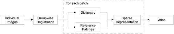
Flowchart of the proposed method. Inputs are the preprocessed individual images, and output is a constructed atlas.

Unbiased Groupwise Registration

All image were preprocessed with the standard procedure which includes resampling, bias correction, skull stripping [Shi et al., 2012], and tissue segmentation [Wang et al., 2011]. The goal of image registration is to spatially normalize all preprocessed subject images into a common space, which is a necessary initial step for subsequent atlas building. Unlike the pairwise registration methods in which a template is always needed, groupwise registration is free of template selection and is able to simultaneously register all subject images onto the hidden common space. Many groupwise registration methods have been developed in the past years [Joshi et al., 2004; Learned‐Miller, 2006; Wu et al., 2012]. In this article, we employ a state‐of‐the‐art groupwise registration method [Wu et al., 2012] for aligning the input images, by using its freely‐available software package at http://www.nitrc.org/projects/glirt. Specifically, this groupwise registration method jointly minimizes the overall image differences between each pair of subject images in the population by using (1) attribute vector as morphological signature of each voxel for guiding accurate correspondence detection among all subject images, and (2) a hierarchical process for selecting a small number of key voxels (with distinctive attribute vectors) to drive the deformation of other less distinctive points. In this way, the groupwise registration performance is better than the conventional group‐mean based registration method [Joshi et al., 2004], especially for the challenging infant brain registration in our project.

Patch‐Based Representation

We employ a patch‐based representation technique for atlas construction, due to two reasons. First, local anatomical structure could be better described in a small patch than in a large brain region. Second, patch size can be optimized to balance the local structure representativeness and global structure consistency. We sample local cubic patches to cover the whole brain image. Specifically, at a given voxel, we can obtain patches $\left\{p_i|i=1,\dots ,N\right\}$ from all $N$ aligned images at the same location. Note that each patch is represented by a vector consisting of $M=s\times s\times s$ features (i.e., intensities), where $s$ is the size of patch at each dimension.

We consider that all local patches are highly correlated and thus define their distance metric as 1 minus the Pearson correlation coefficient [McShane et al., 2002]. The group center of patches is approximated as the group mean of all patches, i.e., $\frac{1}{N}{\displaystyle \sum }_i^N{p}_i$. In this space of patches, some patches may distribute near the group center, while others may distribute far away. Generally, patches near the group center have more agreement in representing the population mean, while patches far‐away from the group center may be outliers and introduce anatomical discrepancies to degrade the representativeness of the atlas. To this end, we select the $K (\le N)$ patches nearest to the group center, referred to as reference patches and denoted as $\left\{y_k|k=1,\dots ,K\right\}$. To formulate the atlas building (or the estimation of intrinsic group‐mean image) as a representation problem, for each to‐be‐estimated patch in the atlas, we require it to represent the common anatomical structure of all $K$ reference patches simultaneously. Note that, the patch will be similar to the median patch when $K=1$.

To achieve the above goal, we need to first build a dictionary for each atlas patch under construction. An initial dictionary can include all patches with same location in all $N$ aligned images as mentioned above, i.e., $D=[p_1,p_2,\dots ,p_N]$. To further overcome the possible registration error, the initial dictionary is extended to include more patches from the neighboring locations, thus providing a sufficient number of elements for powerful representation. In this application, we include 26 immediate neighboring locations. Thus, for each aligned image, we will take totally 27 patches; and from all N aligned images, we will include totally $N\text{'}=27\times N$ patches in the dictionary D.

Then, we can require the reconstructed atlas patch, which is sparsely represented by the coefficient vector $x$ and the dictionary $D$, to be similar to all $K$ reference patches (denoted by $\left\{y_k|k=1,\dots ,K\right\}$) that are the closest to the group mean as mentioned above. This problem can be formulated as the following minimization problem:

$$\widehat{x}=arg \underset{x>0}{\min }\left[{\displaystyle \sum }_{k=1}^K\Vert Dx-y_k{\Vert }_2^2+\lambda \Vert x{\Vert }_1\right]$$ (1)

where $D\in {\mathrm{ℝ}}^{M\times N^{\prime }}$, $x\in {\mathrm{ℝ}}^{N^{\prime }\times 1}$, $y_k\in {\mathrm{ℝ}}^{M\times 1}$, $\lambda \ge 0$. The first term measures the discrepancy between observation $y_k$ and the reconstructed atlas patch $Dx$, and the second term is $L_1$ regularization on the coefficient vector $x$ (also called LASSO) [Tibshirani, 1996]. Sparsity is encouraged in $x$ under LASSO. $\lambda$ is a non‐negative parameter controlling the influence of the regularization term.

Anatomical Features for Structural Representativeness

In the above atlas construction process, each patch contains only intensity features. Using only the intensity measure for patch similarity may be insufficient to deal with the highly convoluted and variable cortex across individuals. It may also lead to anatomical ambiguity in the built atlas. This issue is well known as intensity uncertainty in image registration [Stewart et al., 2004]. Thus, we propose to integrate anatomical features with intensity features to resolve this anatomical ambiguity issue in the atlas building process.

Since gray matter (GM) and white matter (WM) are the two main components of the brain, we employ the segmented GM and WM maps as additional features [Wang et al., 2011]. Specifically, each patch is now represented by a vector consisting of $M^{\text{'}}=3\times M$ features, which include intensities, GM label map, and WM label map, as shown in Figure 2A. Similarity between patches is redefined as the correlation between their respective intensity features, plus also the correlations between their GM as well as WM features. By doing so, the dictionary patches are now comparing with the center patches for both intensity and tissue information to generate a final atlas patch (Fig. 2B). Here, the GM and WM segmentation maps could be the binary maps or probabilistic maps, scaled to 0–255 as did in the intensity images. Note that GM and WM maps are separated, since a single segmentation map containing different label values for GM and WM may lead to the interpolation problem, e.g., averaging the label values of WM and background could lead to a value near the GM. In some situations, the anatomical features may be not available at certain patches. For example, the patches at the cerebellum may not have GM/WM segmentation results in some image processing pipelines where tissue segmentation is only performed on cerebrum [Wang et al., 2011]. In such cases, the intensity feature will be primarily used for these patches.

Figure 2.

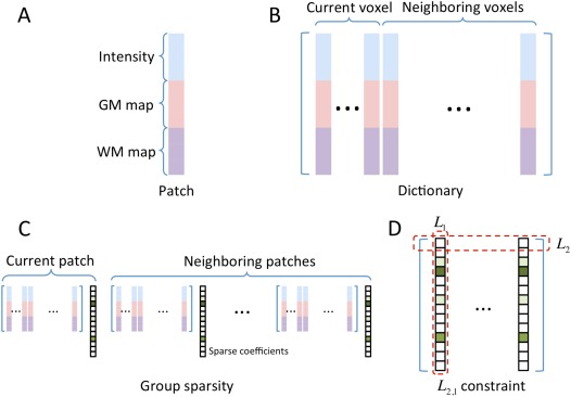
Illustration of the key sparse representation structures in Eq. (2). (A) A patch with dimension of $M\text{'}\times 1$; (B) Dictionary with dimension of $M\prime \times N\prime$; (C) Group sparsity for 1 current patch and 6 neighboring patches; (D) The $L_{2,1}$ constraint on the coefficient matrix with the size of $N\text{'}\times 7$. [Color figure can be viewed in the online issue, which is available at http://wileyonlinelibrary.com.]

Group Regularization on the Neighboring Patches for Spatial Smoothness

Generally, neighboring patches should share similar representations in order to achieve local structure consistency for the constructed atlas. We refer the current patch and its six immediate neighboring patches as a group. Specifically, besides solving the representation task for the current patch, we also consider simultaneously solving the representation tasks for all six immediate neighboring patches, thus constraining the representation coefficients for the entire group (Fig. 2C). To this end, group sparsity regularization, namely group LASSO [Liu et al., 2009], is introduced.

Denote $G=7$ as the total number of patches in the entire group, and let $D_j$, $y_{k,j}$, and $x_j$ denote the respective dictionary, observation variable, and coefficient vector of the jth patch, respectively, with $j=1, 2,\dots ,G$. For simplicity, we use $X=\left[x_1,x_2,\dots ,x_G\right]$ as a matrix containing all column vectors of sparse representation coefficients. Note that the matrix can also be written in the form of row vectors $X=\left[u_1;u_2;\dots ;u_{N^{\prime }}\right]$, where $u_i$ is the ith row in the matrix $X$. Then, we can reformulate the Eq. (1) into a group LASSO problem as below:

$$\widehat{x}=\arg \underset{x>0}{\min }\left[{\displaystyle \sum }_{j=1}^G{\displaystyle \sum }_{k=1}^K\Vert D_j{x}_j-y_{k,j}{\Vert }_2^2+\lambda \Vert X{\Vert }_{2,1}\right]$$ (2)

where $\Vert {X\Vert }_{2,1}={\displaystyle \sum }_{i=1}^{N^{\prime }}\Vert u_i{\Vert }_2$. The first term is a multi‐task least square minimizer for all $G$ neighboring atlas patches under construction. The second term is for regularization. $\Vert {X\Vert }_{2,1}$ is a combination of both $L_2$ and $L_1$ norms, in which the $L_2$ norm is imposed to each row of the matrix $X$ (i.e., $u_i$) to make the neighboring atlas patches have similar sparsity patterns, while the $L_1$ norm is imposed to the all rows of the matrix to ensure the sparsity of representation by the respective dictionary (reflected as the sum of $\Vert u_i{\Vert }_2$) (Fig. 2D). In this way, the nearby patches will share the same sparsity pattern in finding their respective representations. The group LASSO in Eq. (2) can be solved efficiently by using algorithm in [Liu et al., 2009]. The pseudo‐code of the proposed method is given in Algorithm 1.

It is worth indicating that the use of nonoverlapping patches could result in steep gradient changes along patch boundaries and also inconsistent structures across nearby patches. To alleviate this issue, patches are overlapped in atlas construction, and multiple estimations on each location are averaged for obtaining the final atlas information. Specifically, we sample patches in the whole brain by moving the current patch for a half patch size at each time. By doing so, each voxel is now included by multiple patches. Then, by combining all the built overlapped atlas patches together, the final atlas can be obtained.

Algorithm 1

Atlas Construction Using Patch‐based Sparse Representation

Input: N individual Images.

Output: Brain Atlas.

Initialization: All images are preprocessed, tissue‐segmented, and spatially normalized into a common space using groupwise registration. Local cubic patches are sampled to cover the whole brain image.

For each local patch:

1. Construct a vector for each patch in each individual image, including intensity features and the tissue probability maps of GM and WM.

2. Compute a group mean for all N patches at this location, and select K reference patches that are nearest to the group mean.

3. Construct a dictionary D to include the current patch and its 26 immediate neighboring patches.

4. Find a sparse coefficient vector x to represent the K reference patches simultaneously using the dictionary in Eq. (2) for the current and neighboring patches using group regularization.

5. Obtain the resulting atlas patch by multiplying the dictionary ( $D_j$) with the coefficient vector ( ${\widehat{x}}_j$) for the current patch, e.g., $D_j{\widehat{x}}_j$.

End

Obtain the final atlas by averaging the multiple estimations on each local patch.

EXPERIMENTAL RESULTS

Data for Atlas Construction

Neonatal data with low spatial resolution and tissue contrast was used in this study to demonstrate the performance of our detail‐preserving atlas construction method. Specifically, 73 healthy neonatal subjects (42 males and 31 females) were recruited for atlas construction, which were from a large prospective study of early brain development in UNC [Gilmore et al., 2012]. Their MR images were scanned at postnatal 24 ± 10 (9–55) days on a Siemens head‐only 3T scanner. T2‐weighted images were obtained with 70 axial slices using turbo spin‐echo (TSE) sequences at a resolution of 1.25 × 1.25 × 1.95 mm³.

For preprocessing, all images were first resampled into 1 × 1 × 1 mm³. Bias correction was then performed on all images with N3 method [Sled et al., 1998] to reduce the impact of intensity inhomogeneity and thus improve the performance of the subsequent image processing. Non‐brain tissues such as skull and dura were stripped with a learning‐based meta algorithm [Shi et al., 2012]. Finally, brain tissues were segmented into gray matter (GM), white matter (WM), and ventricular cerebrospinal fluid (CSF) using a coupled level‐set algorithm [Wang et al., 2011].

Parameter Setting

Since there is no ground‐truth for the atlas construction, we propose to tune the parameters of our algorithm by measuring the capability of the resulting atlas in spatially normalizing a neonatal population. If the constructed atlas could well represent the anatomy of the population, after alignment, the aligned population will have high structural agreement with each other.

We randomly selected 40 of the 73 images, and used them to construct atlases with different parameter settings. The rest 33 images were aligned to each resulting atlas by using a two‐step procedure, which includes an affine registration using FLIRT in FSL [Jenkinson et al., 2002] and a nonlinear deformable registration using Diffeomorphic Demons [Vercauteren et al., 2009]. Registration parameters in Diffeomorphic Demons were conservatively set as 15 × 10 × 5 for iterations in each of three resolutions, and 2.0 for the strength of smoothing kernel for the deformation field. Brain tissues, i.e., GM, WM, and CSF in segmented images, were also aligned from individual images to the atlas space by applying the same estimated deformation fields. We then calculate the structural agreement between these aligned images to evaluate the representativeness of the generated atlas. To do that, we first generated a mean segmentation image from the aligned population to represent the population‐level common structures, by voxel‐wise majority voting on the aligned segmentation images. Then, this mean segmentation image was compared with each warped individual segmentation image for measuring their structural agreement, by means of Dice Ratio, also referred to as similarity index: $DR=2\left|A{{\displaystyle \cap }}^{}B\right|/\left(\left|A\right|+\left|B\right|\right)$, where A and B are the two segmentations, and DR ranges from 0 (for totally disjoint segmentations) to 1 (for identical segmentations). Note that the structural agreement is not calculated between the atlas and aligned images.

Parameter optimization was performed in an iterative manner [Bach et al., 2012]. Specifically, one parameter was optimized at each time, and when optimizing this parameter, values for other parameters were fixed. Parameters were considered as optimized when no change was found on the iterative results. Figure 3 shows the average Dice Ratio of GM, WM and ventricular CSF as a function of patch size, number of center patches, and regularization parameter $\lambda$. If the patch size is too small, e.g., 2 × 2 × 2, the atlas appears noisy. While if the patch size is too large, e.g., 20 × 20 × 20, its ability of local representation will be affected and the resulting atlas will be blur. Similarly, if the number of reference patches is too small, e.g., $K=2$, the resulting atlas can be easily affected by noise. Results are relatively robust to the variations of regularization parameters. According to these experimental results, we finally set the parameters as below: patch size as 6 × 6 × 6, $K=10$ for reference patches, and regularization parameter as $\lambda =0.01$.

Figure 3.

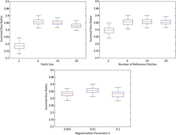
Parameter optimization in constructing infant brain atlas. Forty images were used to construct atlases with different parameters, and 33 images were aligned to each of the constructed atlases. The structural agreement of these aligned images was measured by the average Dice Ratio of GM, WM, and ventricular CSF. [Color figure can be viewed in the online issue, which is available at http://wileyonlinelibrary.com.]

Intermediate Results and Constructed Atlas

Comparison of four different atlas construction methods

Figure 4 compares results obtained with four different atlas construction methods. Top row shows the axial views of the atlases constructed by methods of (a) direct averaging of all images, (b) averaging of 10 center patches, (c) sparse representation, and (d) sparse representation with group constraint. Bottom row shows the close‐up views of the top‐left part of each constructed brain atlas. As we can see, the result obtained from the averaging of 10 center patches (Fig. 4b) shows higher level of details than the result from the direct averaging of all images (Fig. 4a), while it still suffers from steep gradient changes along patch boundaries (or boundary effect) and the inconsistent intensities between neighboring patches. Better structural consistency is observed in the result by sparse representation (Fig. 4c), and further enhanced in the result by using group sparsity (Fig. 4d).

Figure 4.

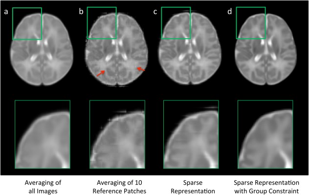
Comparison of atlases built by four different construction methods. The atlases in (b–d) are constructed in a patch‐by‐patch fashion. Steep gradient changes can be observed especially in (b) at the boundaries of nonoverlapping cubic patches, as marked by red arrows. [Color figure can be viewed in the online issue, which is available at http://wileyonlinelibrary.com.]

Importance of anatomical constraint

Anatomical information from GM and WM was employed in our proposed atlas construction framework, when defining the nearest patches and searching for the sparse coefficients. This helps our algorithm to differentiate brain structures so that similar brain structures would be selected together into a more representative atlas. Figure 5 shows the atlases constructed using our proposed method without/with the anatomical constraint. The intensity images of the atlases demonstrate similar appearance, while WM probability map of the proposed method is much clear than that obtained without using anatomical constraint. This indicates that WM is better delineated in our construction of each atlas patch.

Figure 5.

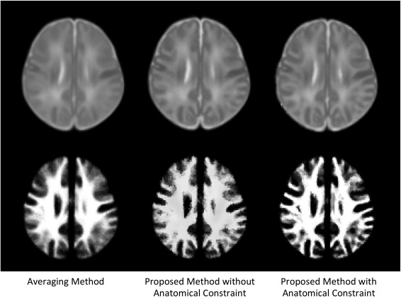
Comparison of atlas construction results by the averaging method and our proposed method without/with anatomical constraint. Top row is the intensity images from the constructed atlases, and the bottom row is WM probability maps.

Influence of the number of training subjects

A question is that how the atlas quality changes as a function of the number of training subjects in this sparse representation process. To explore this, we repeated the atlas construction process by randomly selecting 10 to 73 subjects. Figure 6 shows the close‐up views of intensity images and WM maps of the two representative brain regions. As we can see, results are more affected by registration errors and noise when a small number of subjects were used and thus appear blurry. With the increase of the number of subjects, a clearer pattern of brain anatomy is obtained. In this work, we used all the 73 subjects in atlas construction.

Figure 6.

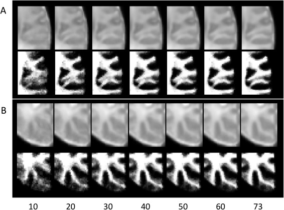
Comparison of atlas construction results with the use of different number of subjects (10 to 73). Two representative brain regions were illustrated in (A) and (B), respectively.

Atlas constructed using all subjects

The atlas constructed using all 73 subjects is shown in Figure 7. From top to bottom are the intensity template, and tissue probability maps of GM, WM, and CSF. From left to right are the six representative axial slices. Note that the complex brain structures, especially in the cortical regions, can be clearly identified from the intensity template, as well as the tissue probability maps.

Figure 7.

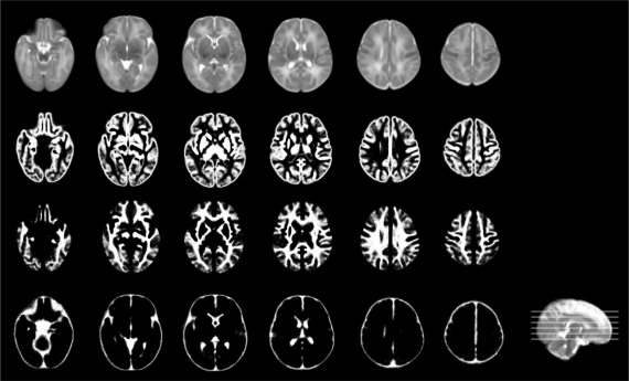
Illustration of the neonatal atlas constructed from 73 subjects using the proposed method. From top to bottom are the intensity atlas, and three tissue probability maps of GM, WM, and CSF. Note that the cerebellum and brain stem are included in the intensity atlas (first row) but excluded in the tissue probability maps [Wang et al., 2011].

Comparison with State‐of‐the‐Art Atlases

Visual inspection

We evaluate the proposed atlas against other state‐of‐the‐art neonatal atlases constructed by different nonlinear registration techniques. Kuklisova‐Murgasova et al. created longitudinal atlases for each week between 28.6 and 47.7 gestational weeks using 142 neonatal subjects [Kuklisova‐Murgasova et al., 2010], and we select their atlas of 41 weeks, referring here as Atlas‐A. Oishi et al. constructed an atlas using 25 brain images from neonates of 0–4 days [Oishi et al., 2011], and we refer it as Atlas‐B. Serag et al [2012] also built longitudinal atlases using 204 premature neonates between 26.7 to 44.3 gestational weeks, in which we select the atlas of 41 weeks and refer here as Atlas‐C. An averaging atlas was also used for comparison, which was constructed by simply averaging our aligned 73 neonate images. Since median is considered as a more robust average over the arithmetic mean [Reuter et al., 2012; Wu et al., 2011], we also generate a median atlas for comparison by selecting the median patches during the atlas construction process. Of note, the Averaging and Median methods were also computed on overlapping patches for fair comparisons with the proposed method. Typical views of these atlases are shown in Figure 8, and their demographic and image acquisition information are listed in Table 1. The proposed atlas, constructed from 73 neonates using sparse representation with group constraints, establishes the highest level of details than any other neonatal atlases. Note that, since the atlases (Atlas‐A, Atlas‐B, and Atlas‐C) were constructed from other datasets, their shapes may seem different with ours (Averaging, Median, and Proposed).

Figure 8.

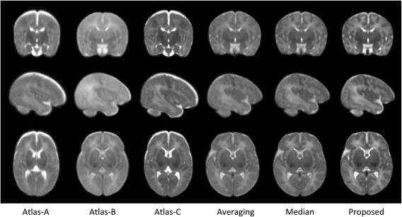
Comparison of neonatal atlases built by Kuklisova‐Murgasova et al. [2010] (Atlas‐A), Oishi et al. [2011] (Atlas‐B), Serag et al. [2012] (Atlas‐C), simple averaging (Averaging), patch‐wise median (Median), and our proposed method (Proposed) on the 73 aligned images. Similar slices were selected from each of these six atlases for easy comparison.

Table 1.

Demographic and T2 image resolution of the neonatal subjects used for atlas construction in the comparison methods

Atlas	No. subjects	Age at MRI scanninga	MR strength	Image resolution (mm3)
Atlas‐A	142 (70 m/72 f)	28.6–47.7 weeks (GA)	3T	0.86 × 0.86 × 1.00
Atlas‐B	25 (15 m/10 f)	0–4 days (PA)	3T	1.88 × 1.88 × 1.88
Atlas‐C	204b	26.7–44.3 weeks (GA)	3T	1.15 × 1.18 × 2.00
Averaging/median/proposed	73 (42 m/31 f)	9–55 days (PA)	3T	1.25 × 1.25 × 1.95

^aGA means gestational age, and PA means postnatal age.

^bGender information was not provided.

Quantitative evaluation

We evaluate the performance of our constructed atlas by comparing with the above‐described neonatal atlases, through the task of spatially normalizing a neonatal population.

In particular, we employed three test datasets that cover the high‐to‐low image resolution (Table 2). Specifically, the test dataset 1 includes eight neonatal images, scanned at postnatal 14 to 58 days on a 3T Siemens scanner with dedicated phased array neonatal head coil [Shi et al., 2011a]. T2 images were obtained with 87 axial slices at a resolution of 1.00 × 1.00 × 1.30 mm³. The test dataset 2 includes 15 neonatal images, with similar scanning parameters to the data used for atlas construction. The test dataset 3 was derived from the healthy neonatal subjects of the online public National Database for Autism Research (NDAR, http://ndar.nih.gov/) [Hall et al., 2012]. Totally 12 subjects were selected with images scanned at postnatal age of 8 to 21 days. T2 images were obtained with 39 axial slices at a resolution of 0.98 × 0.98 × 3.00 mm³. Figure 9 shows the axial slices of six randomly selected subjects from each test dataset.

Table 2.

Demographic and T2 image resolution of the neonatal subjects used in each dataset

	Number	MR strength	Postnatal age at MRI scanning (days)	Image resolution (mm3)
Data for atlas construction	73 (42 m/31 f)	3 T	24 ± 10 (9–55)	1.25 × 1.25 × 1.95
Test dataset 1—high resolution	8 (5 m/3 f)	3 T	24 ± 14 (14–58)	1.00x1.00x1.30
Test dataset 2—normal resolution	15 (8 m/7 f)	3 T	26 ± 6 (14–35)	1.25 × 1.25 × 1.95
Test dataset 3—low resolution	12 (5 m/7 f)	1.5 T	16 ± 3 (8–21)	0.98 × 0.98 × 3.00

Figure 9.

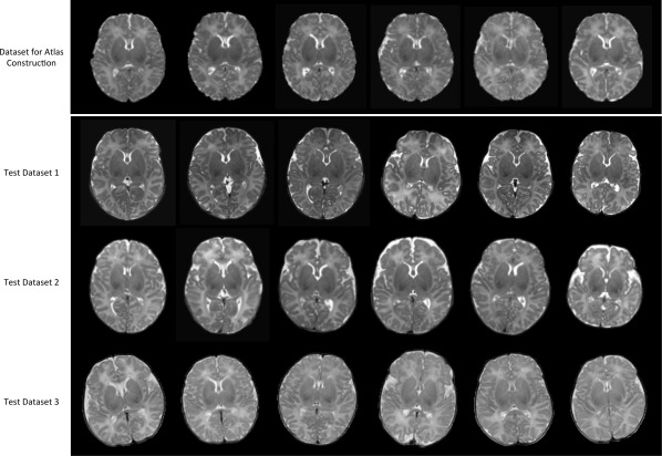
Axial views for the six randomly selected subjects in each of four neonatal datasets. Note that the images in top row were already aligned together and used as the input to our atlas construction method, while images in other three rows are displayed in their native spaces, used for quantitative evaluation.

To quantitatively evaluate our atlas, we also design an experiment to spatially normalize a population of new neonatal images by separately using each of the six atlases shown in Figure 8 as template. In this experiment, we use the three test datasets as detailed above, which are independent of the data used for atlas construction. All images were aligned to each of the six atlases by using first an affine registration with FLIRT in FSL [Jenkinson et al., 2002] and then a nonlinear deformable registration with Diffeomorphic Demons [Vercauteren et al., 2009]. As detailed in the parameter setting subsection, we employ registration parameters of 15 × 10 × 5 for multiscale iterations and 2.0 for the strength of smoothing kernel. Similarly, a mean segmentation image is voted from all individual segmentation images of the aligned testing data, and then compared with each of those individual segmentation images for measuring the mean structural agreement by Dice Ratio.

Statistical analysis results are shown in Figure 10. As can be observed, the atlas constructed by the proposed method outperforms all other atlases in aligning GM and WM tissues (P < 0.01 by two‐sample t‐tests) in all three test datasets. For ventricular CSF, the atlas constructed by the proposed method also has better performance than all other methods in the test datasets 2 and 3, except in the test dataset 1 where no significant difference was found.

Figure 10.

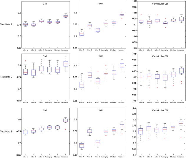
Box plot of the Dice Ratio for the proposed atlas, as well as each of other five comparison atlases. Red lines in the boxes denote the medians, whereas boxes extend to the lower‐ and upper‐quartile values (i.e., 25% and 75%). Whiskers extend to the minimum and maximum values in one‐and‐a‐half interquartile range. Points beyond this range are the potential outliers and thus marked by red “+” symbols. Note that the ventricular CSF was obtained by applying a topological mask [Shi et al., 2011a]. [Color figure can be viewed in the online issue, which is available at http://wileyonlinelibrary.com.]

Computational Time

The program runs under the MATLAB environment on a standard PC using a single thread of an Inter® Xeon® CPU (E5630 1.6 GHz). It takes about 5 h using the selected parameters to process 73 images with the voxel resolution of 1 × 1 × 1 mm³. Note that the atlas construction is performed independently on each patch, thus could be parallelized for saving the computational time on a computer cluster.

DISCUSSION

We have presented a novel patch‐based sparse representation method for atlas construction, with application to the neonatal images. Our contributions are threefold: (1) the atlas is constructed in a patch‐by‐patch fashion, capturing the regionally varying anatomical structures; (2) each patch is sparsely and adaptively represented from an adaptive over‐complete dictionary, promoting the local representativeness; (3) anatomical constraint and group sparsity are adopted for better structural matching and spatial consistency. To the best of our knowledge, the present work is the first of exploring the usage of sparse representation for atlas construction. Experimental results demonstrated that the proposed approach can retain more anatomical details in the constructed neonatal atlas, and the resulting atlas has better abilities for guiding spatial normalization than other three state‐of‐the‐art neonatal atlases, as well as the atlases built with simple averaging or median on our own aligned neonatal data.

It is worth noting that our method is flexible enough to be incorporated with any registration algorithms for further improving the quality of the constructed atlas. Also, our method can be potentially used in any dataset where the atlas quality is affected by large local inter‐subject structural variability, low image resolution, or insufficient tissue contrast, such as in lung images [Li et al., 2012], prostate images [Klein et al., 2008], and mouse brain images [Chuang et al., 2011].

In the application of normalizing a population into a common space, we expect that the atlas would have high representativeness if the aligned population has high structural agreements [Avants et al., 2010; Klein et al., 2010; Shi et al., 2011b]. Note that the requirement of atlas representativeness largely depends on the accuracy of registration methods [Yeo et al., 2008]. In early studies, affine or low degree‐of‐freedom nonlinear registrations are widely used, where the atlas is generally blurry for handling the large amount of inter‐subject structural variability after rough alignment [Ashburner and Friston, 2009; Mazziotta et al., 1995]. As the development of advanced high degree‐of‐freedom nonlinear registration methods [Klein et al., 2009; Wu et al., 2012], atlas is required to have richer local structural details to be better aligned with individual images. For example, as reviewed in [Evans et al., 2012], although the Colin27 T1 atlas is constructed on a single brain with moderated smoothness (averaged from 27 scans), it is widely used by the community for its detailed definition of brain structures. Meanwhile, averaging from 152 subjects, the MNI152 atlas is reproduced recently by using an advanced nonlinear registration method. The resulting atlas is believed having comparable details with the Colin27 atlas with the persevered group representativeness [Evans et al., 2012]. In this article, we proposed a data‐driven method to preserve the local anatomical details from small patches in the process of atlas construction, and experimental results also demonstrated that our atlas achieved better representativeness than other comparison atlases in normalizing the three test datasets with different voxel resolutions.

Our library includes the current patch and its 26 immediate neighbors from all the training subjects. This search neighborhood (3 x 3 x 3) could be enlarged to allow the library for including more neighboring patches, thus leading to potentially a higher representation power. As a trade‐off, this will unfortunately increase the computational load dramatically. A pre‐screening of patches may be effective to reduce the library size and improve the computational efficiency, as employed in non‐local patch studies [Coupé et al., 2011]. We will explore this in the future work. Meanwhile, recent studies proposed that multiple atlases might be a better solution to represent the diversity of data distribution [Blezek and Miller, 2007]. For example, in some applications, subjects were directly used as individual atlases to propagate their label information to a new subject [Gousias et al., 2008; Weisenfeld and Warfield, 2009]. Sabuncu et al. [2009] further extended this idea by generating multiple atlases from the population with a data‐driven method, which equips these atlases with better subgroup representativeness. Thus, the proposed method could also be used in the application of multi‐atlases construction, after defining subgroups from the entire population. This will be definitely our future work.

In our previous work, we constructed a neonatal brain atlas from 95 subjects by using a nonlinear group‐wise registration method [Shi et al., 2011b]. The method used for constructing atlas is the simple averaging as described above (Fig. 8), thus obtaining similar atlas as provided in Figure 8 (for simple averaging). Our proposed method in this article provides a finer atlas than that obtained with simple averaging, as demonstrated by both visual inspection and quantitative measurements in the above. We will release our constructed neonatal atlases as we did before (http://www.med.unc.edu/bric/ideagroup/free-softwares).

REFERENCES

- Ashburner J (2007): A fast diffeomorphic image registration algorithm. Neuroimage 38:95–113. [DOI] [PubMed] [Google Scholar]
- Ashburner J, Friston KJ (2009): Computing average shaped tissue probability templates. Neuroimage 45:333–341. [DOI] [PubMed] [Google Scholar]
- Avants BB, Yushkevich P, Pluta J, Minkoff D, Korczykowski M, Detre J, Gee JC (2010): The optimal template effect in hippocampus studies of diseased populations. Neuroimage 49:2457–2466. [DOI] [PMC free article] [PubMed] [Google Scholar]
- Bach F, Mairal J, Ponce J (2012): Task‐driven dictionary learning. IEEE Trans Pattern Anal Machine Intell 34:791–804. [DOI] [PubMed] [Google Scholar]
- Blezek DJ, Miller JV (2007): Atlas stratification. Med Image Anal 11:443–457. [DOI] [PMC free article] [PubMed] [Google Scholar]
- Brodmann K (1909): Vergleichende Lokalisationslehre der Grosshirnrinde in ihren Prinzipien dargestellt auf Grund des Zellenbaues. Germany: Barth Leipzig. [Google Scholar]
- Chuang N, Mori S, Yamamoto A, Jiang H,Ye X, Xu X, Richards LJ, Nathans J, Miller MI, Toga AW, Sidman RL, Zhang J (2011): An MRI‐based atlas and database of the developing mouse brain. Neuroimage 54:80–89. [DOI] [PMC free article] [PubMed] [Google Scholar]
- Coupé P, Manjón JV, Fonov V, Pruessner J, Robles M, Collins DL (2011): Patch‐based segmentation using expert priors: Application to hippocampus and ventricle segmentation. Neuroimage 54:940–954. [DOI] [PubMed] [Google Scholar]
- Evans AC, Janke AL, Collins DL, Baillet S (2012): Brain templates and atlases. Neuroimage 62:911–922. [DOI] [PubMed] [Google Scholar]
- Fonov V, Evans AC, Botteron K, Almli CR, McKinstry RC, Collins DL (2011): Unbiased average age‐appropriate atlases for pediatric studies. Neuroimage 54:313. [DOI] [PMC free article] [PubMed] [Google Scholar]
- Gilmore JH, Shi F, Woolson SL, Knickmeyer RC, Short SJ, Lin W, Zhu H, Hamer RM, Styner M, Shen D (2012): Longitudinal development of cortical and subcortical gray matter from birth to 2 years. Cerebral Cortex 22:2478–2485. [DOI] [PMC free article] [PubMed] [Google Scholar]
- Gousias IS, Rueckert D, Heckemann RA, Dyet LE, Boardman JP, Edwards AD, Hammers A (2008): Automatic segmentation of brain MRIs of 2‐year‐olds into 83 regions of interest. Neuroimage 40:672–684. [DOI] [PubMed] [Google Scholar]
- Hall D, Huerta MF, McAuliffe MJ, Farber GK (2012): Sharing heterogeneous data: The National Database for Autism research. Neuroinformatics 1–9. [DOI] [PMC free article] [PubMed] [Google Scholar]
- Jenkinson M, Bannister P, Brady M, Smith S (2002): Improved optimization for the robust and accurate linear registration and motion correction of brain images. Neuroimage 17:825–841. [DOI] [PubMed] [Google Scholar]
- Joshi S, Davis B, Jomier M, Gerig G (2004): Unbiased diffeomorphic atlas construction for computational anatomy. Neuroimage 23:151–160. [DOI] [PubMed] [Google Scholar]
- Klein A, Andersson J, Ardekani BA, Ashburner J, Avants B, Chiang M.‐C, Christensen GE, Collins DL, Gee J, Hellier P (2009): Evaluation of 14 nonlinear deformation algorithms applied to human brain MRI registration. Neuroimage 46:786. [DOI] [PMC free article] [PubMed] [Google Scholar]
- Klein A, Ghosh SS, Avants B, Yeo BT, Fischl B, Ardekani B, Gee JC, Mann JJ, Parsey RV (2010): Evaluation of volume‐based and surface‐based brain image registration methods. Neuroimage 51:214–220. [DOI] [PMC free article] [PubMed] [Google Scholar]
- Klein S, van der Heide UA, Lips IM, van Vulpen M, Staring M, Pluim JP (2008): Automatic segmentation of the prostate in 3D MR images by atlas matching using localized mutual information. Med Phys 35:1407–1417. [DOI] [PubMed] [Google Scholar]
- Kuklisova‐Murgasova, M , Aljabar, P , Srinivasan, L , Counsell, S , Doria, V , Serag, A , Gousias, I , Boardman, J , Rutherford, M , Edwards, A (2010): A dynamic 4D probabilistic atlas of the developing brain. Neuroimage 54:2750–2763. [DOI] [PubMed] [Google Scholar]
- Learned‐Miller EG (2006): Data driven image models through continuous joint alignment. Journal IEEE Trans Pattern Anal Machine Intell 28:236–250. [DOI] [PubMed] [Google Scholar]
- Li B, Christensen GE, Hoffman EA, McLennan G, Reinhardt JM (2012): Establishing a normative atlas of the human lung: computing the average transformation and atlas construction. Acad Radiol 19:1368–1381. [DOI] [PMC free article] [PubMed] [Google Scholar]
- Liu J, Ji S, Ye J (2009): Multi‐task feature learning via efficient l2,1‐norm minimization. In Proceedings of the Twenty‐Fifth Conference on Uncertainty in Artificial Intelligence, pp. 339–348. AUAI Press.
- Mazziotta JC, Toga AW, Evans A, Fox P, Lancaster J (1995): A probabilistic atlas of the human brain: theory and rationale for its development. The International Consortium for Brain Mapping (ICBM). Neuroimage 2:89–101. [DOI] [PubMed] [Google Scholar]
- McShane LM, Radmacher MD, Freidlin B, Yu R, Li M‐C, Simon R (2002): Methods for assessing reproducibility of clustering patterns observed in analyses of microarray data. Bioinformatics 18:1462–1469. [DOI] [PubMed] [Google Scholar]
- Miller MI, Beg MF, Ceritoglu C, Stark C (2005): Increasing the power of functional maps of the medial temporal lobe by using large deformation diffeomorphic metric mapping. Proc Natl Acad Sci USA 102:9685–9690. [DOI] [PMC free article] [PubMed] [Google Scholar]
- Oishi K, Mori S, Donohue PK, Ernst T, Anderson L, Buchthal S, Faria A, Jiang H, Li X, Miller MI (2011): Multi‐contrast human neonatal brain atlas: application to normal neonate development analysis. Neuroimage 56:8–20. [DOI] [PMC free article] [PubMed] [Google Scholar]
- Reuter M, Schmansky NJ, Rosas HD, Fischl B (2012): Within‐subject template estimation for unbiased longitudinal image analysis. Neuroimage 61:1402–1418. [DOI] [PMC free article] [PubMed] [Google Scholar]
- Sabuncu MR, Balci SK, Shenton ME, Golland P (2009): Image‐driven population analysis through mixture modeling. IEEE Trans Med Imaging 28:1473–1487. [DOI] [PMC free article] [PubMed] [Google Scholar]
- Serag A, Aljabar P, Ball G, Counsell SJ, Boardman JP, Rutherford MA, Edwards AD, Hajnal JV, Rueckert D (2012): Construction of a consistent high‐definition spatio‐temporal atlas of the developing brain using adaptive kernel regression. Neuroimage 59:2255–2265. [DOI] [PubMed] [Google Scholar]
- Shen D, Davatzikos C (2002): HAMMER: Hierarchical attribute matching mechanism for elastic registration. IEEE Trans Med Imaging 21:1421–1439. [DOI] [PubMed] [Google Scholar]
- Shi F, Wang L, Wu G, Zhang Y, Liu M, Gilmore JH, Lin W, Shen D (2012): Atlas construction via dictionary learning and group sparsity. In Medical Image Computing and Computer–Assisted Intervention–MICCAI, pp. 247–255, Springer, Berlin Heidelberg. [DOI] [PubMed]
- Shi F, Shen D, Yap P‐T, Fan Y, Cheng J‐Z, An H, Wald LL, Gerig G, Gilmore JH, Lin W (2011a): CENTS: Cortical enhanced neonatal tissue segmentation. Hum Brain Mapp 32:382–396. [DOI] [PMC free article] [PubMed] [Google Scholar]
- Shi F, Wang L, Dai Y, Gilmore JH, Lin W, Shen D (2012): LABEL: Pediatric brain extraction using learning‐based meta‐algorithm. Neuroimage 62:1975–1986. [DOI] [PMC free article] [PubMed] [Google Scholar]
- Shi F, Yap P‐T, Wu G, Jia H, Gilmore JH, Lin W, Shen D (2011b). Infant brain atlases from neonates to 1‐ and 2‐year‐olds. PLoS One 6:e18746. [DOI] [PMC free article] [PubMed] [Google Scholar]
- Sled JG, Zijdenbos AP, Evans AC (1998): A nonparametric method for automatic correction of intensity nonuniformity in MRI data. IEEE Trans Med Imaging 17:87–97. [DOI] [PubMed] [Google Scholar]
- Stewart C, Lee Y‐L, Tsai C‐L (2004): An uncertainty‐driven hybrid of intensity‐based and feature‐based registration with application to retinal and lung CT images. In Medical Image Computing and Computer‐Assisted Intervention–MICCAI 2004, pp. 870–877. Springer Berlin Heidelberg.
- Talairach J, Tournoux P (1988): Co‐Planar Stereotaxic Atlas of the Human Brain. New York: Thieme. [Google Scholar]
- Tibshirani R (1996): Regression shrinkage and selection via the lasso. J R Statist Soc 58:267–288. [Google Scholar]
- Tzourio‐Mazoyer N, Landeau B, Papathanassiou D, Crivello F, Etard O, Delcroix N, Mazoyer B, Joliot M (2002): Automated anatomical labeling of activations in SPM using a macroscopic anatomical parcellation of the MNI MRI single‐subject brain. Neuroimage 15:273–289. [DOI] [PubMed] [Google Scholar]
- Vercauteren T, Pennec X, Perchant A, Ayache N (2009): Diffeomorphic demons: Efficient non‐parametric image registration. Neuroimage 45:S61–S72. [DOI] [PubMed] [Google Scholar]
- Vinje WE, Gallant JL (2000): Sparse coding and decorrelation in primary visual cortex during natural vision. Science 287:1273–1276. [DOI] [PubMed] [Google Scholar]
- Wang L, Shi F, Lin W, Gilmore JH, Shen D (2011): Automatic segmentation of neonatal images using convex optimization and coupled level sets. Neuroimage 58:805–817. [DOI] [PMC free article] [PubMed] [Google Scholar]
- Weisenfeld NI, Warfield SK (2009): Automatic segmentation of newborn brain MRI. Neuroimage 47:564–572. [DOI] [PMC free article] [PubMed] [Google Scholar]
- Wu G, Jia H, Wang Q, Shen D (2011): SharpMean: groupwise registration guided by sharp mean image and tree‐based registration. Neuroimage 56:1968–1981. [DOI] [PMC free article] [PubMed] [Google Scholar]
- Wu G, Wang Q, Jia H, Shen D (2012): Feature‐based groupwise registration by hierarchical anatomical correspondence detection. Hum Brain Mapp 33:253–271. [DOI] [PMC free article] [PubMed] [Google Scholar]
- Yang J, Wright J, Huang TS, Ma Y (2010): Image super‐resolution via sparse representation. IEEE Trans Image Process 19:2861–2873. [DOI] [PubMed] [Google Scholar]
- Yeo BTT, Sabuncu MR, Desikan R, Fischl B, Golland P (2008): Effects of registration regularization and atlas sharpness on segmentation accuracy. Med Image Anal 12:603–615. [DOI] [PMC free article] [PubMed] [Google Scholar]
- Zhang S, Zhan Y, Dewan M, Huang J, Metaxas DN, Zhou XS (2012): Towards robust and effective shape modeling: Sparse shape composition. Med Image Anal 16:265–277. [DOI] [PubMed] [Google Scholar]
- Shi F, Wang L, Wu G, Zhang Y, Liu M, Gilmore JH, Lin W, Shen D (2012): Atlas construction via dictionary learning and group sparsity. In Medical Image Computing and Computer‐Assisted Intervention‐MICCAI 2012, pp. 247–255. Springer Berlin Heidelberg. [DOI] [PubMed]
- Shi F, Fan Y, Tang S, Gilmore JH, Lin W, Shen D (2010): Neonatal brain image segmentation in longitudinal MRI studies. Neuroimage 49:391–400. [DOI] [PMC free article] [PubMed] [Google Scholar]
- Wang L, Shi F, Yap P‐T, Lin W, Gilmore JH, Shen D (2011): Longitudinally guided level sets for consistent tissue segmentation of neonates. Human brain mapping.. [DOI] [PMC free article] [PubMed]
- Yap P‐T, Fan Y, Chen Y, Gilmore JH, Lin W, Shen D (2011): Development trends of white matter connectivity in the first years of life. PLOS one, 6(9), e24678. [DOI] [PMC free article] [PubMed] [Google Scholar]
- Fan Y, Shi F, Smith JK, Lin W, Gilmore JH, Shen D (2011): Brain anatomical networks in early human brain development. Neuroimage, 54(3), 1862–1871. [DOI] [PMC free article] [PubMed] [Google Scholar]
- Shi F, Yap P‐T, Fan Y, Gilmore JH, Lin W, Shen D, (2010): Construction of multi‐region‐multi‐reference atlases for neonatal brain MRI segmentation. Neuroimage, 51(2), 684–693. [DOI] [PMC free article] [PubMed] [Google Scholar]
- Yang J, Shen D, Davatzikos C, Verma R (2008): Diffusion Tensor Image Registration Using Tensor Geometry and Orientation Features In: Metaxas D., Axel L., Fichtinger G., Székely G., editors. Medical Image Computing and Computer–Assisted Intervention – MICCAI 2008: Springer Berlin Heidelberg; p 905–913. [DOI] [PubMed] [Google Scholar]
- Zacharaki EI, Shen D, Lee S‐k, Davatzikos C (2008): ORBIT: A Multiresolution Framework for Deformable Registration of Brain Tumor Images. IEEE Transactions on Medical Imaging, 27:1003–1017. [DOI] [PMC free article] [PubMed] [Google Scholar]
- Shen D, Wong W‐h, lp HHS (1999): Affine‐invariant image retrieval by correspondence matching of shapes. Image and Vision Computing, 17:489–499. [Google Scholar]
- Xue Z, Shen D, Davatzikos C (2006): Statistical representation of high‐dimensional deformation fields with application to statistically constrained 3D warping. Medical Image Analysis, 10:740–751. [DOI] [PubMed] [Google Scholar]
- Jia H, Wu G, Wang Q, Shen D (2010): ABSORB: Atlas building by self‐organized registration and bundling. NeuroImage, 51:1057–1070. [DOI] [PMC free article] [PubMed] [Google Scholar]
- Tang S, Fan Y, Wu G, Kim M, Shen D (2009): RABBIT: Rapid alignment of brains by building intermediate templates. NeuroImage, 47:1277–1287. [DOI] [PMC free article] [PubMed] [Google Scholar]
- Yap P‐T, Wu G, Zhu H, Lin W, Shen D (2009): TIMER: Tensor Image Morphing for Elastic Registration. NeuroImage, 47:549–563. [DOI] [PMC free article] [PubMed] [Google Scholar]