Extracting and summarizing white matter hyperintensities using supervised segmentation methods in Alzheimer's disease risk and aging studies

Abstract

Precise detection and quantification of white matter hyperintensities (WMH) observed in T2‐weighted Fluid Attenuated Inversion Recovery (FLAIR) Magnetic Resonance Images (MRI) is of substantial interest in aging, and age‐related neurological disorders such as Alzheimer's disease (AD). This is mainly because WMH may reflect co‐morbid neural injury or cerebral vascular disease burden. WMH in the older population may be small, diffuse, and irregular in shape, and sufficiently heterogeneous within and across subjects. Here, we pose hyperintensity detection as a supervised inference problem and adapt two learning models, specifically, Support Vector Machines and Random Forests, for this task. Using texture features engineered by texton filter banks, we provide a suite of effective segmentation methods for this problem. Through extensive evaluations on healthy middle‐aged and older adults who vary in AD risk, we show that our methods are reliable and robust in segmenting hyperintense regions. A measure of hyperintensity accumulation, referred to as normalized effective WMH volume, is shown to be associated with dementia in older adults and parental family history in cognitively normal subjects. We provide an open source library for hyperintensity detection and accumulation (interfaced with existing neuroimaging tools), that can be adapted for segmentation problems in other neuroimaging studies. Hum Brain Mapp 35:4219–4235, 2014. © 2014 Wiley Periodicals, Inc.

INTRODUCTION

Focal white matter (WM) changes associated with aging and diseases of the central nervous system are common and are often labeled as white matter hyperintensities (WMH) because of their bright appearance on transverse relaxation (T2‐weighted) or fluid attenuated inversion recovery (FLAIR) magnetic resonance (MR) image sequences [Goldberg and Ransom, 2003, Maillard et al., 2012]. In the context of normal aging as well as cerebrovascular diseases and neurodegenerative disorders, such as Alzheimer's disease (AD), WMH may reflect ischemic injury and contribute to cognitive decline in aging [Au et al., 2006; Yoshita et al., 2006] and portend progression to dementia due to AD [Brickman et al., 2012; Carmichael et al., 2010; Debette et al., 2010]. They may be an early indicator of white matter neurodegenerative change, amyloid angiopathy, or be primarily ischemic in nature [Maillard et al., 2012]. Their presence in the context of AD, particularly when cognitive symptoms are mild, is variable and their relative contribution to explaining the mechanism of cognitive loss in AD remains unclear [Brickman et al., 2012; Jellinger, 2002]. In contrast, in the context of multiple sclerosis (MS) or other demyelinating disease, the presence of hyperintensities is typically viewed as pathognomonic, representing inflammatory lesions, and may be indicative of disease phase and predictive of cognitive outcome [Filippi et al., 2011]. Because WMH are commonly observed in aging individuals that are ostensibly cognitively normal, it has been proposed that these may be indicative of subclinical cerebrovascular disease [Luchsinger et al., 2009]. Further, it has been proposed that the extent of WMH burden adversely affects an individual's brain resilience to other disease such as AD [Brickman et al., 2011; Meier et al., 2012], a devastating neurodegenerative disorder affecting 1 in 10 older adults over age 65. Thus, the careful quantification of WMH may improve the prediction of AD, and a better understanding of WMH occurrence may yield mechanisms to prolong brain health in people who acquire additional brain disease. For this reason, in the last few years, efforts seeking to precisely extract and quantify WMH volume and tie their occurrence to the temporal course and severity of AD and related disorders have attracted substantial interest in the neuroimaging community [Debette and Markus, 2010; Ramirez et al., 2011; Smith et al., 2011; Yoshita et al., 2006].

At its core, the WMH extraction task described above is an image segmentation problem, a fundamental topic of research in computer vision. A number of recent articles have successfully applied vision algorithms for identifying WMH [Admiraal‐Behloul et al., 2005; Anbeek et al., 2004; Geremia et al., 2011; Kruggel et al., 2008; Ong et al., 2012; Schmidt et al., 2011], albeit this body of literature focuses overwhelmingly on identifying MS pathologies from the images. For the MS application, these methods have been validated on benchmark datasets, mostly yield satisfactory performance, and have been translated into end user software [Schmidt et al., 2011] (http://www.applied-statistics.de/lst.html). While in principle, these algorithms should be extendable to the task of identifying hyperintensities independent of the disorder under study, it is not obvious whether existing algorithms will perform sufficiently well when the lesions are small, diffuse, or otherwise irregular in shape or intensity, which are characteristics of subtle or emerging ischemic lesions seen in the context of cerebrovascular disease and aging. Even among WMH identified in a single image, we empirically find that there may be sufficient heterogeneity in characteristics that leads to unsatisfactory misclassification of some small or diffuse lesions using the existing standard methods for reasons that go much beyond mere parameter adjustment.

This article is motivated by the problem described above, and focuses on new strategies for reliable identification and extraction (i.e., segmentation) of WMH in studies centered on mild cognitive impairment (MCI), AD, cardiovascular risk, and other aging‐related disorders. To put this goal in context, we must highlight its need relative to the state of the art in image processing and certain properties of this specific application. First, observe that segmentation algorithms from computer vision, in general, are fundamentally designed to detect globally conspicuous or salient regions of interest from natural images [Forsyth and Ponce, 2011]. This assumption applies to most widely used segmentation functions such as Markov Random Fields [Boykov et al., 2001], Normalized Cuts [Shi and Malik, 2000], Random Walks [Grady, 2006], as well as spatial adaptations of clustering objective functions [Comaniciu and Meer, 2002]. WMH in AD may be small in size and their structure is occasionally elongated (spatially aligned with lateral ventricles). Further, they may not have a strong image gradient which makes visual identification of these regions from the background quite problematic. In summary, while this is still a segmentation task, it does not satisfy the basic assumptions that make standard segmentation objectives directly applicable. As the regions of interest become less salient and difficult to pick out (especially for a nonexpert), the use of common segmentation algorithms incrementally becomes more problematic. Note that it is not the effectiveness of these “unsupervised” segmentation functions per se, rather their appropriateness for the task at hand.

In this article, we argue that accurate segmentations of WMH in AD imaging studies can significantly benefit from user supervision provided a priori in the form of training data (i.e., expert indications)—to specify characteristics of the regions we seek to extract. A few explorations of this idea have been undertaken before [Gaonkar et al., 2010; Lao et al., 2008], however, these works made limited use of only image intensity and histogram based features. It turns out that features based on rich textural and perceptual (structural) characteristics of WMH, to be presented shortly, yield significant benefits beyond intensity features, and provide reliable detection mechanisms that generalize well even when the underlying imaging protocol changes. We argue that with a suitable set of image processing based features that extract this structural information, a state of the art supervised algorithm can “learn” the relevant characteristics to be able to identify/classify WMH and non‐WMH pixels in new unseen MR images in a reliable manner. When actualized, this allows incorporating expert knowledge within segmentation to significantly improve sensitivity to hyperintensities and reproducibility of detection.

The proposed methods are based on training data that was generated via interactive hand indications by an expert. A suite of image processing steps (described in the next section) are then adopted to distill various perceptual summaries of WMH regions. Utilizing these measures as features within a supervised framework, the core learning module models classifiers trained to distinguish between WMH and non‐WMH pixels. On unseen MR images, the classifiers can accurately segment WMH regions in a completely automated manner. We present empirical evidence showing the efficacy of the proposed methods on three distinct medium sized datasets, and compare it with the state of the art. The key contributions of this article are:

1. It is demonstrated via an extensive set of experiments that reliable segmentation of white matter hyperintensities in AD risk studies is possible via adaptations of supervised learning methods on an appropriately constructed set of features. The training process is simple to execute.

2. An easy to use software library (interfaced with SPM12, a widely used neuroimaging tool) is provided, for adoption of these segmentation methods within neuroimaging analyses in AD as well as studies focused on other disorders.

This article is organized as follows. Methodology section briefly outlines the theory of the supervised learning models adopted here—specifically, Support Vector Machines (SVM) and Random Forests (RF). This is followed by the various image processing modules that comprise the actual detection process. Experimental Setup section evaluates segmentation results of the two models, SVM and RF, against training data (an existing lesion segmentation tool serves as a baseline for these comparisons). We also present results of a statistical analysis of WMH quantifications relative to several clinically‐based cardiovascular risk biomarkers. Discussion section interprets and sheds additional light on our empirical findings. Also we briefly summarize the features of the open source library accompanying this manuscript, and finally Conclusion section concludes the article.

METHODOLOGY

Before going into the details of our detection framework, we first provide a high level overview of the key modules involved in segmentation process. We formulate the task of White Matter Hyperintensities (WMH) segmentation as a supervised inference problem. In other words, prior knowledge of the physical characteristics of these hyperintensities is incorporated into our segmentation algorithm via a learning procedure on a small set of input images (using available expert indicated segmentations). We construct texton based features from the imaging data, and then learn a classifier (based on Support Vector Machines and Random Forests) which assigns varying weights to those features that best discriminate WMH and non‐WMH voxels. With a learned model in hand, our segmentation task boils down to evaluating a probability estimate of whether a voxel is WMH or not, given the parameters of the classifier. Both models offer distinct advantages in the context of estimating the conditional probabilities—shortly, we will discuss their relative benefits before moving to evaluating their performance.

Preprocessing

An important physical characteristic of WMH is they appear to be hyperintense on T2‐fluid attenuated inversion recovery (T2‐MR) images. On the other hand, they tend to be fairly dark on T1‐weighted (T1‐MR) scans as shown in Figure 1. This suggests that using both T1‐MR and T2‐MR (i.e., multichannel information) to model WMH will be beneficial. To do this, we first coregister T2‐MR to T1‐MR and then apply multichannel tissue segmentation to extract GM, WM, and CSF partial volume estimates (PVE). SPM12b (http://www.fil.ion.ucl.ac.uk/spm) was used to construct the PVEs. Bias correction to the coregistered T2‐MR is applied before constructing a region of interest (ROI) using WM PVE. It has been observed that several regions lying on the boundaries of ventricles are miss‐segmented as GM and/or CSF. Hence we extract a ventricular template from CSF PVE and adjust the ROI to include these periventricular regions. Figure 2 gives a schematic overview of the preprocessing pipeline. The input to our detection module is the extracted ROI.

Figure 1.

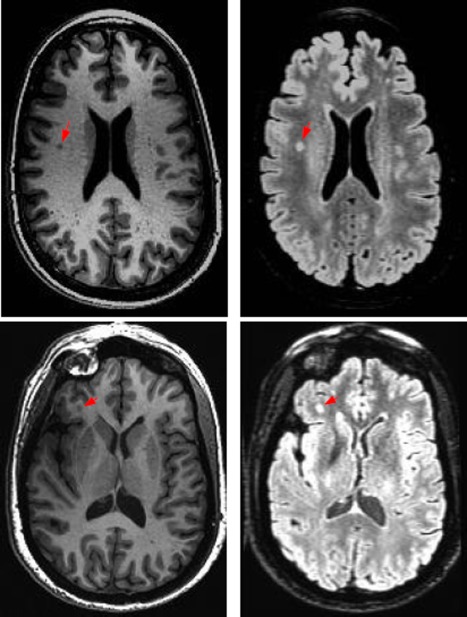
T1 and T2 images of two subjects showing varying visual characteristics of lesions in the different modalities. [Color figure can be viewed in the online issue, which is available at http://wileyonlinelibrary.com.]

Figure 2.

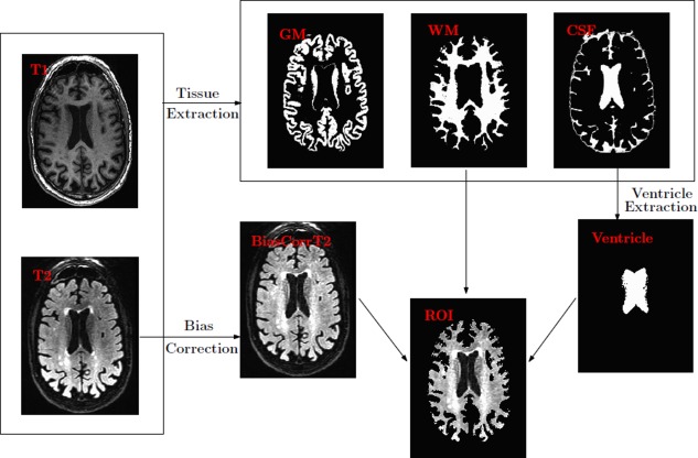
Preprocessing pipeline. WM and CSF PEVs from T1‐MR and coregistered (and bias corrected) T2‐MR are used to construct the ROI. [Color figure can be viewed in the online issue, which is available at http://wileyonlinelibrary.com.]

Feature Extraction

To characterize the low‐level localized context around each voxel, we extract texture and intensity‐variation based features using standard image processing filtering operations. In particular, we use texture filters referred to as textons [Leung and Malik, 2001; Malik et al., 1999] which are an ensemble of low, high and band pass spatial filters. A low pass filter extracts smoothness of intensities across voxels, band pass filters encode the partial volume effect, whereas high pass and edge filters pick up boundaries and edges. Overall, the set of filters we use are (a) baseline low‐pass filter; (b) baseline high‐pass filter; (c) ensemble of band‐pass filters; (d) edge filter. All these responses are concatenated into a feature vector (constructed for each voxel). Figure 3 gives an overview of this feature construction process. For each voxel v in the ROI, a neighborhood “patch” I(v) is extracted. This three‐dimensional matrix is then convolved with a kernel (corresponding to the texton filters above). Gaussian and Laplacian kernels are used for low and high pass filters respectively. Band‐pass filters constitute a “pyramid” of difference of Gaussians and Laplacians [De Bonet, 1997; Leung and Malik, 2001; Malik et al., 1999]. The edge filter used Sobel detection maps Lee et al. [1987]. The concatenated response to all these filters (referred to as textons) characterize the voxel intensities, localized intensity variations as well as the texture of the patch I(v). Depending on the number of texton filters n _f, and the size of patch Lv, we construct a n _f Lv length feature vector for each voxel of interest. Figure 4 illustrates texture‐based feature responses for WMH voxels and non‐WMH voxels (randomly selected across several image slices). Compare the strong inter‐cluster similarities between the filter responses of WMH voxels (in blue) versus those of non‐WMH voxels (in black) which appear to be diffuse and show high variance. Our next goal is to exploit the clustering behavior seen in Figure 4 within a classifier, so the determination of whether a voxel is WMH/non‐WMH can be performed automatically at segmentation time. Details on filter parameters like kernel type, bandwidth and variance are provided in the project documentation.

Figure 3.

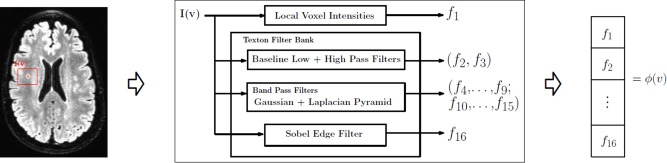
Feature extraction. For each vowel, v, a patch I(v) is used to construct the features. f ₁ gives the intensity variation inside I(v) and f ₂…, f ₁₆ represent the textural information. The final feature vector is ϕ(v). By its contribution ϕ(v) is 16 times the number of voxels in I(v). Note that I(v) is three‐dimensional. [Color figure can be viewed in the online issue, which is available at http://wileyonlinelibrary.com.]

Figure 4.

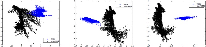
Filter bank responses. Low pass, high pass, and band pass texton responses for a set of 8,000 voxel centers (equally split between WMHs and non‐WMHs) depicting a definitive structure of WMHs (the blue cluster) versus the more diffuse and irregular fabric of non‐WMHs (in black). [Color figure can be viewed in the online issue, which is available at http://wileyonlinelibrary.com.]

Learning Algorithms

The machine learning methods we utilize in our framework are Support Vector Machines (SVM) and Random Forest (RF). We provide a brief self‐contained overview here and refer the reader to Cortes and Vapnik [1995], Schölkopf and Smola [2001], Breiman [2001] for more details.

Support vector machines (SVM)

The SVM model solves for a hyperplane that separates the data points (or their high dimensional representation). Other than merely finding any hyperplane that offers separability, SVM seeks to divide the classes maximally—that is, the hyperplane should have a large margin to each class (which gives good generalization capability). In WMH segmentation, we have a two class problem with labels denoted as y _i, i = 1, …, N where +1 gives the WMH class and −1 gives the non‐WMH class. Further, N denotes the training data size—in other words, the number of voxels whose class label is already known. Denote the vector of filter responses as x_i. Using widely available solvers, we optimize the model in Eq. (1), where C controls how heavily misclassification will be penalized. The kernel K is analogous to a similarity matrix, which denotes how similar example xi is to example x_j. Once the variables α _i are calculated, the prediction for a test feature sample x is simply given by Σ_i (α _iy_iK(x,x_i) − b). Sign of the prediction denotes the WMH/non‐WMH class (±1) and magnitude represents the confidence level (i.e., the prediction can be treated as a signed distance),

$$\underset{{\alpha }_i}{\max }{\displaystyle \sum _{i=1}^N{\alpha }_i-\frac{1}{2}}{\displaystyle \sum _{i,j}{\alpha }_i{\alpha }_j}{y}_i{y}_j\mathcal{K}\left(x_i,x_j\right)\mathrm{s.t.}{\displaystyle \sum _{i=1}^N{\alpha }_i{y}_i=0,0\le {\alpha }_i\le C}$$ (1)

Random forest (RF)

The second learning model used in our framework is the Randomized Decision Trees. RF construct a large number of independent decision trees based on random subspace selection of training features. Let R represent the number of trees to be constructed and F denote the training feature set. A 2‐class RF design is shown in Figure 5. We first select a random subset of features, and then grow a binary tree by picking a smaller fraction of features within the selected feature set, and choosing a split‐point at each tree level. The best threshold (split point) is the one which favors homogeneity within each child node (low impurity) and heterogeneity across them. The output from the training procedure is an ensemble of trees. Prediction of class membership for new examples is performed by evaluating inter and intra tree variability (instead of maximal class separation), that is, the mean of individual tree outputs. This design extends easily to the regression setting where the output is any real number between −1 and +1.

Figure 5.

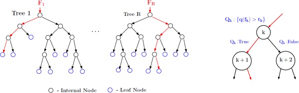
Random forest design. A total of R trees are designed. F ₁,…., F _R are the feature subsets (with replacement) used to construct the respective tree. For the rth tree, at node k, a query Q _k is asked about the data f _k ∊ F _r and depending on the result the data f _k is split into two parts. Each tree is grown to the maximum resulting in pure leaf nodes (data belong to a single class). [Color figure can be viewed in the online issue, which is available at http://wileyonlinelibrary.com.]

Training

We use the above methods to learn a WMH classifier from preprocessed T2‐MR images. To generate the training data, we need a precise characterization of local visual appearance of both WMH and non‐WMH voxels. To this end, we used hand‐indications from an expert who scanned through all images in our dataset and marked out all the WMH regions. Since this is a very tedious process especially if the image has many small sized WMH and introduces unintended error at the boundaries with low intensity contrast, we used a semisupervised Random Walker based segmentation method [Grady, 2006] to facilitate the indications. Here, the user marks many foreground/background seed points and incrementally interacts with the segmentation method until the results are considered satisfactory. The traced out WMH regions are checked for accuracy in a second session to ensure that no WMH are missed, and we obtain good training data with accurate boundary delineation. Our training data must consist of both positively and negatively labeled examples. A large number of patches centered on WMH voxels serve as positive training examples, whereas patches randomly derived from other regions serve as negative training examples for the training set.

Obtaining the Final WMH Segmentation

Once the training process has been completed and the SVM/RF classifier has been obtained, for a given to‐be‐segmented FLAIR image I, we apply the model(s) to obtain a voxel‐level class‐specific labeling of the image. The two methods investigated are following the description in 2.3 SVM based classification and RF based regression. Note that regression setting of RF, though theoretically similar to the classification, provides flexibility in terms of the outputs being continuous. The range of segmentation outputs depend on the method utilized. (i) SVM outputs are signed distance maps where positive values indicate WMH and negative indicate non‐WMH. (ii) RF (regression) outputs are empirical distributions ranging from −1 (WMH) to 1 (non‐WMH). Each of these outputs are then converted into class‐wise probabilities via logistic regression [Bewick et al., 2005] providing the desired WMH segmentation “maps” (refer to Fig. 6). These final WMH segmentations are probability maps in [0, 1], and denote the likelihood that a given voxel is hyperintense.

Figure 6.

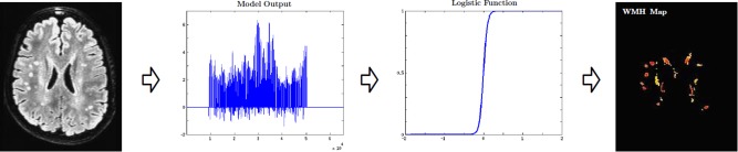
Final WMH segmentation maps. Depending on the method used the segmentation outputs are either distance maps (SVM) or empirical distributions (RF). The final WMH map is obtained by registering these outputs. Range of the final WMH maps is [0, 1] with 0 denoting a non‐WMH, and 1 a WMH. [Color figure can be viewed in the online issue, which is available at http://wileyonlinelibrary.com.]

The total WMH burden (along with deep and periventricular accumulations) in the form of raw voxel count is used for analysis in several neurological studies [Au et al., 2006; Kruit et al., 2010; Vermeer et al., 2003]. Our probability map outputs allow us to calculate a per subject WMH burden which we call a normalized Effective WMH Volume (EV), and can serve as a useful summary measure. The EV measure is calculated as,

$$\text{EV}=\frac{{\displaystyle {\sum }_{z}P{\left(z\right)}^{k}D\left(z\right)}}{\text{ICV}}\hspace{1em}\text{where}\hspace{1em}D\left(z\right)=\{\begin{array}{cc}\begin{array}{c}1\\ 0\end{array}& \begin{array}{c}P\left(z\right)>\gamma \\ \text{else}\end{array}\end{array}$$ (2)

where P(z) is the output probability map and ICV is the intracranial (or brain) volume [Keihaninejad et al., 2010]. D(z) is an indicator function that nullifies any voxels with WMH probability smaller than 0 < γ < 1. A low value of γ (generally <0.25) ensures the removal of low‐confidence (presumably noisy) voxels while summarizing the accumulation. k ≥ 1 is an integer. Hence EV calculates the hyperintense voxel count “weighted” by the corresponding likelihood (where k controls the degree of the weight). This scalar summary can now be used in additional analyses, as discussed shortly. Note that the normalization by ICV accounts for the differences in brain sizes, hence making EV an unbiased estimator of hyperintensity burden. Periventricular (pEV) and deep (dEV) hyperintensity accumulations can be calculated using the ventricular template (estimated in the process during preprocessing, refer to Fig. 2) as follows,

$$\text{pEV}={\displaystyle \sum _z\text{EV}\left(z\right)}R\left(z\right);\text{dEV}={\displaystyle \sum _z\text{EV}\left(z\right)}\left(1-R\left(z\right)\right)$$ (3)

where R(z) is 1 if voxel z belongs to periventricular region. Although there are several definitions that delineate deep white matter from periventricular, we follow the construction used in [DeCarli et al., 2005a].

Experimental Setup

Subjects and data

For experimental evaluations of our proposed methods, we utilized T1‐MR and T2‐MR scans from a total of 251 subjects (male: 114, female: 137). This data comes from one of the several studies conducted at Wisconsin Alzheimer's Disease Research Center (WADRC). All scans were acquired on a GE 3T scanner with eight‐channel coil. Table 1 lists the relevant imaging protocol parameters. Our cohort included 169 healthy controls (CN) (age in years: 46–91, median: 61.7), 40 mild cognitively impaired (MCI) (age in years: 53–89, median: 75.4), and the remainder were demented (AD) (age in years: 58–95, median: 75.5). The criteria for MCI (amnestic single or multidomain) and AD followed from standard published clinical criteria [Albert et al., 2011; McKhann et al., 2011]. A validation is done from an expert panel of dementia specialists (which included two of the co‐authors C.M.C. and S.C.J.). All of the subjects had at least 8 years of education. 62 carried at least one copy of Apolipoprotein E (APOE) e4 allele. Among the 169 CN, 131 had parental Family History (FH) (52 maternal, 39 paternal, and 40 both) of AD, ascertained from review of the parent medical records including autopsy results (if available).

Table 1.

Data acquisition protocol parameters

Parameter	Tl	T2‐FLAIR
Matrix (pixels)	256 × 256	256 × 256
Number of Slices	156	100
Thickness (mm)	1	2
FOV (Percent Phase)	100	90
Repetition Time	8.16	6000
Echo Time	3.18	122.95
Inversion Time	450	1869
Flip Angle	12	90
Pulse Sequence	IR‐SPGR	CUBE

Evaluations setup

We evaluated the performance of our methods by comparing the voxel‐wise WMH/non‐WMH class predictions with respect to training data. Apart from comparisons with respect to expert indications, we used the Lesion Segmentation Toolbox (LST) [Schmidt et al., 2011] (which is currently the state of the art for this task) as a baseline. LST constructs lesion belief maps using Markov Random Field (MRF) based lesion growing. These lesion belief maps are initialized by thresholding voxel intensities for GM, WM, and CSF. Voxel intensities are used to update the likelihoods. Please refer to [Schmidt et al., 2011] for complete details. For these experiments, training was performed on a random sample of 38 T2‐MR images and testing was done with leave‐one‐out cross‐validation (with multiple realizations). We ensured consistency across the comparisons by applying the same preprocessing pipeline (refer to Table 2) to both our methods as well as LST. A total of 16 textons were used in our experiments. For each voxel of interest a 2,000 long feature vector was constructed using 5 × 5 × 5 neighborhood. Misclassification tolerance of SVM model (C) was set to 1, and the number of trees R for RF was 50. We provide complete details of our parameter values (e.g., error tolerance, feature subset size and impurity indices of RF) in the project documentation. Empirically we found that LST was sensitive to κ (in [0, 1]), the threshold for initializing belief maps, which is set heuristically. However, the algorithm performs an internal selection process to provide an “optimal” κ (hereafter referred to as LST_opt). We used this automated threshold as well as a wide range of manual thresholds (10 of them) to setup a fair set of comparisons which were designed to assess overall segmentation performance enhancement of our models over the current solutions. It should be observed that, although comparing supervised segmentation methodology to an unsupervised technique is not “traditional,” the main purpose of these evaluations is to prove the necessity of supervised methods (and not to present a new supervised detection). k = 1 and γ = 0.25 in all the experiments.

Table 2.

SPM12 preprocessing parameters

Co‐registration
Objective function	NMI
Sampling distance	4 × 2
Smoothing distance	7 × 7
Interpolation	Trilinear
Tissue Segmentation
Bias regularization	10−4
Bias FWHM	120 mm
Coregistration	SPM default
Processing space	Native

The performance measures include precision‐recall (PR) and dice coefficient‐recall (DR) curves [Arbelaez et al., 2011; Manning et al., 2008]. F‐measure (not to be confused with F‐statistic) and average precision (AP), calculated from the PR curves, are used to summarize the overall segmentation performance of each method [Manning et al., 2008]. F‐measures inherently assume equal importance to both false positives (FP) and false negatives (FN). Hence, in addition, we evaluated F_0.5‐measures (and F₂‐measures respectively) which summarize the PR curves when FN are assumed to be half (and twice respectively) as important as FP. Also a hypothetical summary measure, break even point (BEP) is reported, which can be interpreted as the “best” possible operating point of the method is reported [Manning et al., 2008]. It is important to note that the number of WMH voxels (true‐positives, TP) is far smaller (on the order of 10⁻⁴) compared with the non‐WMH voxels (true negatives, TN) in an image. Therefore, it is meaningless to report raw accuracy measures (which yield >99% accuracy independent of method). The above described PR curve based measures turn out to be more meaningful in this case. For further details, see Manning et al. [2008].

Secondary statistical analysis

Recall that the accumulation of hyperintensities across white matter has significant correlation with age and dementia status [Barber et al., 1999; Debette and Markus, 2010; Smith et al., 2008] of middle‐aged and older adults. Further there have been studies that investigate the relationship of family history (FH) to the hyperintensity burden in cognitively healthy subjects. Having constructed a hyperintensity accumulation, EV, we investigate the efficacy of this summary measure in revealing similar statistical dependencies. To this end, the following statistical tests are conducted. (A) EV versus age − monotonicity of EV with increasing age, (B) EV versus dementia, controlled for age − differences of mean and rate of change of accumulation with respect to age, across CN, MCI and AD, (C) EV versus FH for cognitively healthy subjects − group differences of mean EV. Note that the empirical distribution of accumulations is not normal. To maintain consistency across all the three analyses, a power transformation is applied over EV. More details about the analysis setup for each of the three cases (characteristics of the data, etc.) will be presented in Discussion section while discussing the results. Observe that the segmentation performance was assessed using the 38 subjects who had training data, while the statistical analysis was conducted using accumulations from all the 251 subjects.

RESULTS

Figure 7 and Table 3 summarize the performance comparison of SVM and RF (along with the baseline LST) against ground truth. PR and DR curves of SVM, RF and LSTopt are shown in Figure 7(a,b). The corresponding performance summaries (i.e. F, AP, BEP, F_0.5, and F₂) are shown in Table 3. Observe that RF‐based regression performed the best with F = 0.672, AP ∼ 0.8 and BEP = 0.678. LSTopt, as expected (being unsupervised), performed the worst (F = 0.410 and AP = 0.350). Following the described in Evaluation setup section, 10 different t s are used for LST (including an optimal one), all chosen meaningfully by visual validation. The corresponding PR curves and maximum F values are shown in Figure 7c,d. LSTs F values ranges from 0.392 to 0.426 much smaller then that of RF, and the maximum (0.426) did not correspond to the optimal choice used by the toolbox (0.410). Figure 8 shows the detections of our best method, RF on six different image slices with varied hyperintensity structures (from large and contiguous to small and diffuse). The last two images are of particular interest where there were false positives (along the cortical regions fourth column) and false negatives (along periventricular WMH boundaries − last column). None of the images in Figure 8 had any expert indications. Figure 9 presents the effectiveness of supervised methods, as claimed in Introduction section, in segmenting small and diffuse (irregular) hyperintensities. It compares the postprocessed segmentation outputs (i.e. probability maps) to both the expert indications and LSTopt on three different images. Observe that LST performs very poorly, and SVMs outputs seem to be over segmented compared with RF. Note that all the image overlays in Figures 8 and 9 are produced in AFNI with a overlay threshold of 0.5. Following comparison against multiple t s of LST as in Figure 7c,d, Figure 10 presents LST outputs at three different t s (one of which is the optimal t chosen by the toolbox) to that of SVM and RF. Figure 11 and Table 4 show the results of our secondary statistical analysis. Firstly, the interaction of age and dementia had a significant (P < 0.01, F = 6.56) dependence on accumulation. Secondly, both the accumulation volume and its rate of change (with increasing age) were found to be different for CN, MCI, and AD groups (refer to Fig. 11a). Further, there was a significant dependence of hyperintensity burden on parental family history with P = 0.02, F = 3.34. The subjects with maternal and both FH had more hyperintensity accumulation (1.63 ± 1.15 and 0.88 ± 0.45 respectively) than those with paternal and no FH (0.78 ± 0.40 and 0.73 ± 0.30 respectively).

Figure 7.

Precision versus recall (PR) curves, dice coefficient versus recall (DR) curves and F measures. (a) PR curves of LST_opt, SVM, and RF. (b) DR curves of LST_opt, SVM, and RF. (c) PR curves with differential initial thresholds k (including the optimal one) of LST. (d) Comparison of change in F‐measures across the multiple LST implementations (of c) with respect to that of SVM and RF. Color map for LST, SVM, and RF is blue, black, and red, respectively. Observe that the results of LST_opt are sensitive to the hyperparameter k, and the performance does not improve by changing it. These results show the improved performance of our methods over existing best unsupervised segmentation method. [Color figure can be viewed in the online issue, which is available at http://wileyonlinelibrary.com.]

Table 3.

Performance of LST_opt, SVM, and RF methods against expert indications

Method	Model	F	AP	BEP	F0.5	F2
LSTopt	MRF	0.410	0.350	0.414	0.412	0.504
sc	Classification	0.540	0.565	0.534	0.558	0.626
RR	Regression	0.672	0.797	0.678	0.685	0.763

F‐measure (also referred to as Dice Coefficient) is the (maximum) of the ratio of 2TP to 2TP+FP+FN. AP (which is equivalent to the area Tinder Precision Recall curve) and BEP summarize the effectivity of each method in minimizing both FP and FN simultaneously. F_0.5 and F ₂ penalize FP over FN and FN over FP, respectively. RF‐based regression was the best with highest AP, F_0.5, and F ₂ values.

Figure 8.

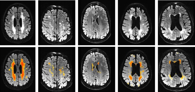
Example segmentation outputs of RF. These results show that RF method performs well both in picking up at large contiguous as well as small irregular hyperintensity regions. Fourth column shows an example of over segmentation (along cortical regions) and the last column shows a case of false negatives. The color map overlays range from blue (0) to red (1). [Color figure can be viewed in the online issue, which is available at http://wileyonlinelibrary.com.]

Figure 9.

Three example segmentation results compared with expert indications and LST_opt. Each row corresponds to one subject. First column shows the FLAIR image. Second column present the expert indications overlayed onto the FLAIR. Third and fourth columns correspond to the SVM and RF outputs (final probability maps). The last column presents the LST_opt. Observe that the number of false negatives are very few, if not none, both for SVM and RF outputs, and there are a few false positives. The color map of overlays ranged from blue (0) to red (1). [Color figure can be viewed in the online issue, which is available at http://wileyonlinelibrary.com.]

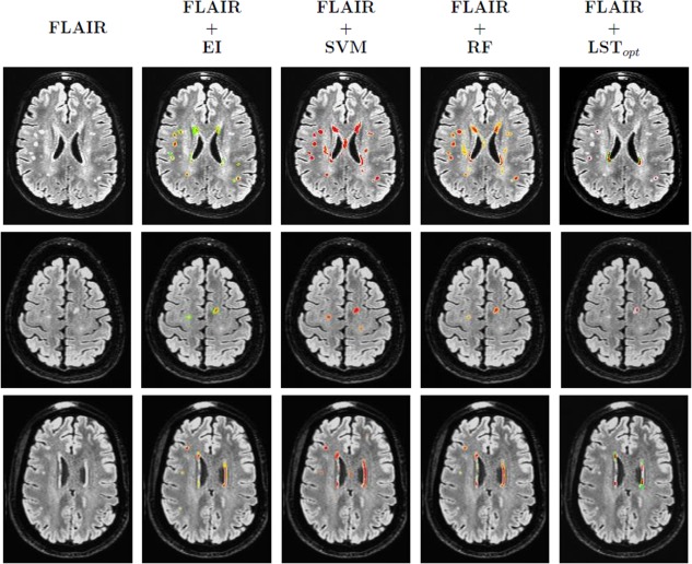
Figure 10.

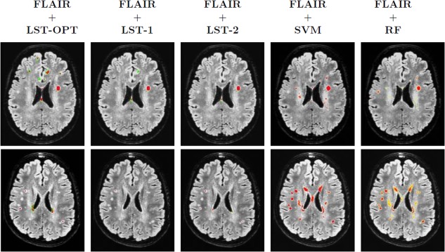
Sensitivity of LST outputs to k. Each row corresponds to one subject. First three columns are the LST outputs at different ks (optimal k chosen by toolbox followed by k = 0.1 and k = 0.2, respectively). Last two columns correspond to the outputs of SVM and RF, respectively. Underlays are coregistered and bias corrected FLAIR images and the color map of overlays range from blue (0) to red (1). [Color figure can be viewed in the online issue, which is available at http://wileyonlinelibrary.com.]

Figure 11.

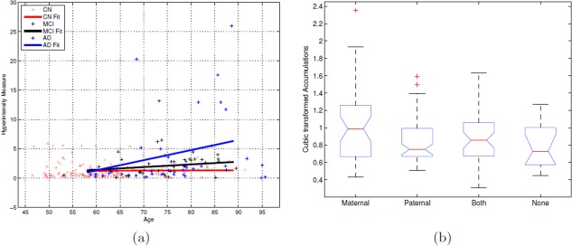
(a) Linear regression fits of EV versus age for each of the three groups CN, MCI, and AD. The slope (rates) for CN fit was almost constant and AD fit was the highest. And at a given age, as expected, AD subjects had more accumulation than MCI and CN. (b) ANOVA box plot for transformed accumulation versus FH. There was significant difference across the four groups (P = 0.02, F = 3.34), with maternal and both FH subjects having higher EVs compared with paternal and none. On each box, the central mark is the median, the edges of the box are the 25th and 75th percentiles and the whiskers extend to ±2.5 standard deviations. [Color figure can be viewed in the online issue, which is available at http://wileyonlinelibrary.com.]

Table 4.

Confidence levels (i.e., mean and standard deviations) of accumulations for CN, MCI, and AD groups at four difference ages along with the rates of change (slopes of linear fit)

Dementia status	Slope of linear fit	Age
		60	70	80	85
CN	0.004	1.24 ±0.51	1.27 ±0.63	1.30 ±1.04	1.31 ±1.28
MCI	0.03	1.30 ±1.21	1.88 ±1.22	2.33 ±1.24	2.56 ±1.68
AD	0.17	1.42 ±1.19	3.05 ±1.18	4.78 ± 1.09	5.64 ±1.37

The accumulation is smallest for CN (and remained almost the same with increasing age), followed by MCI and much higher for AD.

DISCUSSION

The foremost observations from our results is that RF based regression performs best with F = 0.672, AP = 0.797 and BEP = 0.678 (refer to Table 3). Good F and AP indicate that the number of FP are low, which is supported by F _0.5 = 0.685. Also F ₂ = 0.763 and BEP is almost the same as F which shows that RF method penalizes both the FN and FP equally strongly (indicating a balanced minimization of false classifications) while recovering the TP. Figure 9 shows the effectivity of RF is picking up small and diffuse regions, the main characteristic of a hyperintense region, as described in Introduction section. SVM, however was worse compared with RF, with F = 0.540 and AP = 0.565. This is not surprising as SVM tends to over segment (being liberal) the hyperintensities (for examples refer to Fig. 9), since the output of a SVM is margin (distance from the class‐separating hyperplane) and that of RF is an empirical distribution (bounded within [0, 1]). Hence the number of FP (including extra boundaries as shown in Fig. 9) in the case of SVM will be much higher than that of RF. Note that the F (and the F _0.5, F ₂ measures) in Table 3 are based on the PR curves of Figure 7a and represent the maximum of the harmonic mean of precision and recall [Manning et al., 2008]. Figure 7b shows the change in this F‐measure (i.e., Dice coefficient) as a function of recall (i.e., sensitivity). Observe that both RF has consistently best F values as recall is varied from 0 to 1.

To understand the variability in segmentation performance of RF refer to Figure 8 where five different images (not from the training/cross‐validated set) are shown. As shown in the first three columns of Figure 8, RF does good job in picking up long and contiguous regions (which are characteristics of periventricular WMH in demented subjects, and subjects who had stoke), as well as small and diffuse deep hyperintensities. Fourth and fifth columns show two cases involving false detections, where several cortical regions (fourth column) are detected and boundaries along periventricular hyperintensities (fifth column) are missed. The reason of these false segmentations is mainly due to high non‐uniformity of intensity bias along the scan, and it should be observed that these artifacts have to be corrected for during preprocessing (the segmentation module implicitly cannot correct for such errors). Although most of the noisy detections, especially along the cortical surfaces and boundaries of white and grey matter tissues are removed by a postprocessing step (refer to obtaining the final WMH segmentation section). Also, the number of trees learned by RF did not have any influence on the performance of detection (This observation is not random or specific to the problem at hand, but follows from their theory [Breiman, 2001], which shows that sufficiently large number of trees do exceedingly well in picking up the structural characteristics of a given data distribution).

LST outputs (as described in Evaluation setup section) were found to be highly sensitive to its initial threshold, t. While occasionally, manual adjustment of t on an image by image basis led to some improvements, overall the results showed no compelling improvement. Figure 10 illustrates this observation, where LST outputs of two subjects (once corresponding to diffuse and small hyperintensities and the other more contiguous) at three different t s. The results improved for the image in top column (where the hyperintensity is contiguous and large in size) as the threshold t varied from its optimum. However, the results deteriorated for the second case where the regions are very small and highly diffuse in terms of their intensity variation. This suggests that LST picked up conspicuous hyperintensities missing many of the smaller ones (independent of the chosen t). Figure 7c,d compares the PR curves and the resulting F‐measures for 10 different t s where no noticeable improvement was observed in overall detection performance (maximum F‐measure was 0.409, with median equal to 0.380). These observations (missing much of the WMH of interest and sensitivity to t) arise due to the nature of LSTs learning model, which is a lesion growing algorithm using Markov Random Fields (MRF) [Schmidt et al., 2011]. Its initialization (which depends on the initial threshold t) is heuristic and the growth rate parameters are iteratively solved. Such unsupervised segmentation algorithms [Boykov et al., 2001] work reasonably well when the region of interest is large/conspicuous, with significant image gradient or contrast variation from background pixels. However, WMHs in older populations, may not always have these characteristics, and may instead exhibit some differences (relative to non‐WMH regions) in the texture representation. Our results suggest that this textural (structural) information, when appropriately characterized by sufficient training data, yields improved segmentation performance with reliable detections (Table 3). The computational time required for our method was approximately 35 min per subject (this was the same as LST). Although the time taken for generating training data is subjective to the expert generating them and the image being segmented, the approximate time per subject is under 45 min. Note that the time for expert indications is only part of training, and not testing.

The supervised modeling considered here is further validated by performing a secondary statistical analysis of the clinical significance of our summary measure EV (as described in Secondary statistical analysis section). Before interpreting these results it should be noted that, our main aim here is to support existing relationships (already reported [Barber et al., 1999; Debette and Markus, 2010; Smith et al., 2008]) of hyperintensity accumulation to age, dementia status, and/or family history (for dementia). Although, in the process we indicate comparisons that need more detailed analysis (both in terms of choice of modeling and independent/dependent variables). A significant correlation of age was observed with EV, with P < 10⁻⁴ and Spearman Correlation value of 0.29. Note that EV is a “true” summary of accumulation since the differences in brain volume is already accounted for [refer to Eq. (2)] making the summaries. Hence comparing raw values of EVs across subjects is valid for the purpose of any downstream analysis. k = 1, γ = 0.5 and ICV measured in cubic milliliters is for all these validations.

The mean age of CN subjects was 61.14 which is much lower than that of MCI (75.4) and AD (75.5). Hence to evaluate the interaction of age and dementia status on the hyperintensity accumulation, a linear regression (i.e. a linear fit) of EV and age was performed independently for each of the three groups (CN, MCI and AD). Figure 11a shows these three linear fits. Note that no transformation of any type has been applied to the accumulations [derived using Eq. (2)].Though the minimum and maximum ages in our cohort are 46 and 95, the line fits are only considered from 58 to 89. This is because outside this range, at least one of the three groups (CN, MCI, AD) has no subjects. Firstly, Figure 11a shows that the slopes of the three linear fits were found to be different (CN < 0.005, MCI = 0.03, AD > 0.16). The hyperintensity accumulation rate of MCI (AD respectively) subject was ~4 (~32 respectively) times to that of CN with increase in age. Also the mean accumulations (line fit values) of AD were consistently higher than that of MCI and CN. The precise differences in the mean EVs between the three groups (along with the standard deviations) are shown in Table 4 for ages of 65, 75, and 85. Observe that the mean EV for an AD subject is much higher than that of MCI and CN at a given age. The mean and rate of increase of EV was found to be approximately constant in the age range under consideration. Although this might be a data artifact (the number of CN subjects who are older than 70 was smaller than those who are younger). These results suggest that not only does the hyperintensity accumulation increase as a subject grows older, but this rate of change is high for MCI, and much higher for AD groups, than that of healthy ones. For completion, an analysis of covariance was performed indicating the significance of the interaction term (status × age) with a P < 0.01 and F statistic of 6.56. Finally, ANOVA (analysis of variance) was conducted on EV against FH among cognitively normal subjects (169 in number). The four groups of FH include subjects with maternal, paternal, both and none dementia. A cubic power transformation was applied to EVs so that their empirical distribution will be approximately normal. The group difference was significant with P = 0.02 and F = 3.34 (refer to the ANOVA table in Fig. 11b). The four subjects with maternal FH (1.63 ± 1.15) were found to have highest accumulation (in the nontransformed domain) followed by those with both (0.88 ± 0.45), paternal (0.78 ± 0.40), and no (0.73 ± 0.30) FH in that order. Note that the y‐axis in Figure 11b is in power transformed domain. It should be observed that the efficacy of statistical analysis has a direct correlation to that of segmentation accuracy of a given model. Hence, a statistical analysis done using LST (which performs worse than our method, refer to Fig. 7 and Table 3) would be expected to be inaccurate in detecting the dependency of hyperintensity burden to both age and dementia status.

Limitations

The limitation of region growing based algorithms discussed above is a shared characteristic of many automated unsupervised learning methods. Specifically, segmentation methods based on Gaussian distribution/curve fitting (followed by thresholding) [Brickman et al., 2009, 2011; DeCarli et al., 2005b; de Boer et al., 2009], template matching and thresholding [Au et al., 2006; Carmichael et al., 2010] (which are most popular AD risk and aging studies) are susceptible to these limitations. On the other hand, our methods are supervised and therefore can suitably exploit expert indications. But since the textural (structural) information provided by such data is domain dependent, the performance of our methods may be unsatisfactory if the training and testing (prediction) data is inaccurate or come from completely unrelated imaging (MRI) protocols (to the point that the extracted texture features are meaningless). Also, in our procedure, the preprocessing is almost entirely done by SPM12, and any errors in white matter tissue segmentation will propagate into the classifier. Hence, the user intervention involved in training data generation (and evaluation of its quality) and the reliability of preprocessing can be seen as limitations of the proposed model.

Wisconsin WMH Segmentation Toolbox

We provide a MATLAB based implementation of our algorithms. The toolbox, which we refer to as W2MHS (Wisconsin WMH Segmentation Toolbox) is available for download from NITRC, Source Forge as well as from http://pages.cs.wisc.edu/~vamsi/w2mhs.html. This tool interfaces with SPM12, a widely used neuroimaging software and builds upon its preprocessing module. The implementation encompasses the best supervised method, RF based regression and provides as output the segmented probability maps as well as EV summaries (total, periventricular and deep) for use in a downstream analysis. The inputs to the tool are T1‐weighted and T2‐FLAIR images, though the individual modules can be adapted for other segmentation tasks as well. Additional options are provided for incorporating new ground truth data. Although SVM was not found to be the best model, the toolbox provides options for implementing SVM based classification too. Exhaustive details about preprocessing criteria, texton filter bank parameters (kernel types, bandwidths, variances, etc.), constants of SVM and RF models (misclassification rate, number of trees, impurity indices, etc.), are provided in the documentation (included in the download link apart from the scripts). The default parameters are set in a way where the segmentations are reasonable, however, we give the user the capability to modify them, if desired, by explicitly explaining the role of each of the parameter. Detailed instructions about downloading installing the library (including a few supporting libraries) and the naming notations (of files) can be found in the documentation as well.

CONCLUSION

We investigated the task of detecting and quantifying White Matter Hyperintensities (WMH) observed in T2 FLAIR images of subjects with the risk of neurological disorders, especially Alzheimer's disease. We posed the problem as supervised inference, and using texture based features we evaluated three different segmentation methods derived from Support Vector Machines and Random Forests. Through extensive simulations we showed that the Random Forest based regression works the best with significant improvement over the current state‐of‐the‐art unsupervised model. Our evaluations also highlighted the importance of user supervision in the form of expert indications for segmenting hyperintensities. Further, we described a summary measure of hyperintensity accumulation, referred to as normalized Effective WMH Volume and validated its efficacy using age, dementia and family history. Finally, this article is accompanied with an open source implementation (interfaced with widely used tools) for segmenting and quantifying hyperintensities, which can be adapted to segmentation tasks in aging and other neuroimaging studies.

ACKNOWLEDGMENTS

The authors thank Jia Xu for discussions and help with a preliminary version of the implementation.

REFERENCES

- Admiraal‐Behloul F, Van Den Heuvel DMJ, Olofsen H, Van Osch MJP, Van der Grond J, Van Buchem MA, Reiber JHC (2005): Fully automatic segmentation of white matter hyperintensities in MR images of the elderly. Neuroimage 28:607–617. [DOI] [PubMed] [Google Scholar]
- Albert MS, DeKosky ST, Dickson D, Dubois B, Feldman HH, Fox NC, Gamst A, Holtzman DM, Jagust WJ, Petersen RC, Snyder PJ, Carrillo MC, Thies B, Phelps CH (2011): The diagnosis of mild cognitive impairment due to Alzheimers disease: Recommendations from the National Institute on Aging‐Alzheimers Association workgroups on diagnostic guidelines for Alzheimer's disease. Alzheimers Dement 7:270–279. [DOI] [PMC free article] [PubMed] [Google Scholar]
- Anbeek P, Vincken KL, van Osch MJP, Bisschops RHC, van der Grond J (2004): Probabilistic segmentation of white matter lesions in MR imaging. Neuroimage 21:1037–1044. [DOI] [PubMed] [Google Scholar]
- Arbelaez P, Maire M, Fowlkes C, Malik J (2011): Contour detection and hierarchical image segmentation. IEEE Trans Pattern Anal Mach Intell 33:898–916. [DOI] [PubMed] [Google Scholar]
- Au R, Massaro JM, Wolf PA, Young ME, Beiser A, Seshadri S, D'Agostino RB, DeCarli C (2006): Association of white matter hyperintensity volume with decreased cognitive functioning: The Framingham heart study. Arch Neurol 63:246. [DOI] [PubMed] [Google Scholar]
- Barber R, Scheltens P, Gholkar A, Ballard C, McKeith I, Ince P, Perry R, OBrien J (1999): White matter lesions on magnetic resonance imaging in dementia with lewy bodies, alzheimers disease, vascular dementia, and normal aging. J Neurol 67:66–72. [DOI] [PMC free article] [PubMed] [Google Scholar]
- Bewick V, Cheek L, Ball J (2005): Statistics review 14: Logistic regression. Crit Care 9:112–118. [DOI] [PMC free article] [PubMed] [Google Scholar]
- Boykov Y, Veksler O, Zabih R (2001): Fast approximate energy minimization via graph cuts. IEEE Trans Pattern Anal Mach Intell 23:1222–1239. [Google Scholar]
- Breiman L. (2001): Random forests. Mach Learn 45:5–32 [Google Scholar]
- Brickman AM, Muraskin J, Zimmerman ME (2009): Structural neuroimaging in Alzheimer's disease: do white matter hyperintensities matter? Dialogues Clin Neurosci 11:181. [DOI] [PMC free article] [PubMed] [Google Scholar]
- Brickman AM, Siedlecki KL, Muraskin J, Manly JJ, Luchsinger JA, Yeung LK, Brown TR, DeCarli C, Stern Y (2011): White matter hyperintensities and cognition: Testing the reserve hypothesis. Neurobiol Aging 32:1588–1598. [DOI] [PMC free article] [PubMed] [Google Scholar]
- Brickman AM, Provenzano FA, Muraskin J, Manly JJ, Blum S, Apa Z, Stern Y, Brown TR, Luchsinger JA, Mayeux R (2012): Regional white matter hyperintensity volume, not hippocampal atrophy, predicts incident Alzheimer disease in the community. Arch Neurol 69:1621‐1627. [DOI] [PMC free article] [PubMed] [Google Scholar]
- Carmichael O, Schwarz C, Drucker D, Fletcher E, Harvey D, Beckett L, Jack CR Jr, Weiner M, DeCarli C; Alzheimer's Disease Neuroimaging Initiative (2010): Longitudinal changes in white matter disease and cognition in the first year of the Alzheimer disease neuroimaging initiative. Arch Neurol 67:1370. [DOI] [PMC free article] [PubMed] [Google Scholar]
- Comaniciu D, Meer P (2002): Mean shift: A robust approach toward feature space analysis. IEEE Trans Pattern Anal Mach Intell 24:603–619. [Google Scholar]
- Cortes C, Vapnik V (1995): Support vector networks. Machine Learn 20:273–297. [Google Scholar]
- de Boer R, Vrooman HA, van der Lijn F, Vernooij MW, Ikram MA, van der Lugt A, Breteler MMB, Niessen WJ (2009): White matter lesion extension to automatic brain tissue segmentation on MRI. Neuroimage 45:1151–1161. [DOI] [PubMed] [Google Scholar]
- De Bonet JS (1997): Multiresolution Sampling Procedure for Analysis and Synthesis of Texture Images SIGGRAPH '97. New York, NY, USA: ACM Press; pp 361–368. [Google Scholar]
- Debette S, Markus HS (2010): The clinical importance of white matter hyperintensities on brain magnetic resonance imaging: Systematic review and meta‐analysis. Br Med J 341:3666. [DOI] [PMC free article] [PubMed] [Google Scholar]
- Debette S, Beiser A, DeCarli C, Au R, Himali JJ, Kelly‐Hayes M, Romero JR, Kase CS, Wolf PA, Seshadri S (2010): Association of MRI markers of vascular brain injury with incident stroke, mild cognitive impairment, dementia, and mortality: The Framingham offspring study. Stroke 41:600–606. [DOI] [PMC free article] [PubMed] [Google Scholar]
- DeCarli C, Fletcher E, Ramey V, Harvey D, Jagust WJ (2005a): Anatomical mapping of white matter hyperintensities (wmh) exploring the relationships between periventricular WMH, deep WMH, and total WMH burden. Stroke 36:50–55. [DOI] [PMC free article] [PubMed] [Google Scholar]
- DeCarli C, Massaro J, Harvey D, Hald J, Tullberg M, Au R, Beiser A, DAgostino R, Wolf PA (2005b): Measures of brain morphology and infarction in the Framingham Heart Study: Establishing what is normal. Neurobiol Aging 26:491–510. [DOI] [PubMed] [Google Scholar]
- Filippi M, Rocca MA, De Stefano N, Enzinger C, Fisher E, Horsfield MA, Inglese M, Pelletier D, Comi G (2011): Magnetic resonance techniques in multiple sclerosis: The present and the future. Arch Neurol 68:1514. [DOI] [PubMed] [Google Scholar]
- Forsyth DA, Ponce J (2011): Computer Vision: A Modern Approach. NJ, USA: Prentice Hall. [Google Scholar]
- Gaonkar B, Erus G, Bryan N, Davatzikos C (2010): Automated segmentation of brain lesions by combining intensity and spatial information In: Biomedical Imaging: From Nano to Macro, 2010 IEEE International Symposium; IEEE Press, Piscataway, NJ, USA. pp 93–96. [Google Scholar]
- Geremia E, Clatz O, Menze BH, Konukoglu E, Criminisi A, Ayache N (2011): Spatial decision forests for MS lesion segmentation in multi‐channel magnetic resonance images. Neuroimage 57:378–390. [DOI] [PubMed] [Google Scholar]
- Goldberg MP, Ransom BR (2003): New light on white matter. Stroke 34:330–332. [DOI] [PubMed] [Google Scholar]
- Grady L (2006): Random walks for image segmentation. IEEE Trans Pattern Anal Mach Intell 28:1768–1783. [DOI] [PubMed] [Google Scholar]
- Jellinger KA (2002): Alzheimer disease and cerebrovascular pathology: An update. J Neural Transm 109:813–836. [DOI] [PubMed] [Google Scholar]
- Keihaninejad S, Heckemann RA, Fagiolo G, Symms MR, Hajnal JV, Hammers A (2010): A robust method to estimate the intracranial volume across MRI field strengths (1.5 T and 3T). Neuroimage 50:1427–1437. [DOI] [PMC free article] [PubMed] [Google Scholar]
- Kruggel F, Paul JS, Gertz HJ (2008): Texture‐based segmentation of diffuse lesions of the brain's white matter. Neuroimage 39:987–996. [DOI] [PubMed] [Google Scholar]
- Kruit MC, Van Buchem MA, Launer LJ, Terwindt GM, Ferrari MD (2010): Migraine is associated with an increased risk of deep white matter lesions, subclinical posterior circulation infarcts and brain iron accumulation: the population‐based MRI CAMERA study. Cephalalgia 30:129–136. [DOI] [PMC free article] [PubMed] [Google Scholar]
- Lao Z, Shen D, Liu D, Jawad AF, Melhem ER, Launer LJ, Bryan RN, Davatzikos C (2008): Computerassisted segmentation of white matter lesions in 3D MR images, using support vector machine. Acad Radiol 15:300. [DOI] [PMC free article] [PubMed] [Google Scholar]
- Lee J, Haralick R, Shapiro L (1987): Morphologic edge detection. IEEE Robot Automation 3:142–156,. [Google Scholar]
- Leung T, Malik J (2001): Representing and recognizing the visual appearance of materials using threedimensional textons. Int J Comput Vis 43:29–44. [Google Scholar]
- Luchsinger JA, Brickman AM, Reitz C, Cho SJ, Schupf N, Manly JJ, Tang MX, Small SA, Mayeux R, DeCarli C, Brown TR (2009): Subclinical cerebrovascular disease in mild cognitive impairment. Neurology 73:450–456. [DOI] [PMC free article] [PubMed] [Google Scholar]
- Maillard P, Carmichael O, Harvey D, Fletcher E, Reed B, Mungas D, DeCarli C (2012): FLAIR and diffusion MRI signals are independent predictors of white matter hyperintensities. AJNR Am J Neuroradiol 34:54‐61. [DOI] [PMC free article] [PubMed] [Google Scholar]
- Malik J, Belongie S, Shi J, Leung T (1999): Textons, contours and regions: Cue integration in image segmentation. In: Proceedings of the Seventh International Conference on Computer Vision, Vol. 2 IEEE Computer Society, Washington, DC, USA. pp 918–925. [Google Scholar]
- Manning CD, Raghavan P, Schütze H (2008): Introduction to Information Retrieval. New York, NY, USA: Cambridge University Press. [Google Scholar]
- McKhann GM, Knopman DS, Chertkow H, Hyman BT, Jack CR Jr, Kawas CH, Klunk WE, Koroshetz WJ, Manly JJ, Mayeux R, Mohs RC, Morris JC, Rossor MN, Scheltens P, Carrillo MC, Theis B, Weintraub S, Phelps CH (2011): The diagnosis of dementia due to Alzheimers disease: Recommendations from the National Institute on Aging‐Alzheimers Association workgroups on diagnostic guidelines for Alzheimer's disease. Alzheimers Dement 7:263–269. [DOI] [PMC free article] [PubMed] [Google Scholar]
- Meier IB, Manly JJ, Provenzano FA, Louie KS, Wasserman BT, Griffth EY, Hector JT, Allocco E, Brickman AM (2012): White matter predictors of cognitive functioning in older adults. J Int Neuropsychol Soc 18:414. [DOI] [PMC free article] [PubMed] [Google Scholar]
- Ong KH, Ramachandram D, Mandava R, Shuaib IL (2012): Automatic white matter lesion segmentation using an adaptive outlier detection method. Magn Reson Imaging 30:807–823. [DOI] [PubMed] [Google Scholar]
- Ramirez J, Gibson E, Quddus A, Lobaugh NJ, Feinstein A, Levine B, Scott CJM, Levy‐Cooperman N, Gao FQ, Black SE (2011): Lesion explorer: A comprehensive segmentation and parcellation package to obtain regional volumetrics for subcortical hyperintensities and intracranial tissue. Neuroimage 54:963–973. [DOI] [PubMed] [Google Scholar]
- Schmidt P, Gaser C, Arsic M, Buck D, Forschler A, Berthele A, Hoshi M, Ilg R, Schmid VJ, Zimmer C, Hemmer B, Muhlau M (2011): An automated tool for detection of FLAIR‐hyperintense white‐matter lesions in multiple sclerosis. Neuroimage 59:3774–3783. [DOI] [PubMed] [Google Scholar]
- Schölkopf B, Smola AJ (2001): Learning With Kernels: Support Vector Machines, Regularization, Optimization, and Beyond. Cambridge, MA, USA: MIT Press. [Google Scholar]
- Shi J, Malik J (2000): Normalized cuts and image segmentation. IEEE Trans Pattern Anal Mach Intell 22:888–905. [Google Scholar]
- Smith EE, Egorova S, Blacker D, Killiany RJ, Muzikansky A, Dickerson BC, Tanzi RE, Albert MS, Greenberg SM, Guttmann CRG (2008): Magnetic resonance imaging white matter hyperintensities and brain volume in the prediction of mild cognitive impairment and dementia. Arch Neurol 65:94–100. [DOI] [PubMed] [Google Scholar]
- Smith EE, Salat DH, Jeng J, McCreary CR, Fischl B, Schmahmann JD, Dickerson BC, Viswanathan A, Albert MS, Blacker D, Greenberg SM (2011): Correlations between MRI white matter lesion location and executive function and episodic memory. Neurology 76:1492–1499. [DOI] [PMC free article] [PubMed] [Google Scholar]
- Vermeer SE, Hollander M, van Dijk EJ, Hofman A, Koudstaal PJ, Breteler M (2003): Silent brain infarcts and white matter lesions increase stroke risk in the general population. Stroke 34:1126–1129. [DOI] [PubMed] [Google Scholar]
- Yoshita M, Fletcher E, Harvey D, Ortega M, Martinez O, Mungas DM, Reed BR, DeCarli CS (2006): Extent and distribution of white matter hyperintensities in normal aging, MCI, and AD. Neurology 67:2192–2198. [DOI] [PMC free article] [PubMed] [Google Scholar]