Exciton dynamics in chromophore aggregates with correlated environment fluctuations

Abstract

We study the effects of correlated molecular transition energy fluctuations in molecular aggregates on the density matrix dynamics, and their signatures in the optical response. Correlated fluctuations do not affect single-exciton dynamics and can be described as a nonlocal contribution to the spectral broadening, which appears as a multiplicative factor in the time-domain response function. Intraband coherences are damped only by uncorrelated transition energy fluctuations. The signal can then be expressed as a spectral convolution of a local contribution of the uncorrelated fluctuations and the nonlocal contribution of the correlated fluctuations.

I. INTRODUCTION

Molecular aggregates constitute the core building blocks of the photosynthetic solar-to-electric energy conversion apparatus, which is made of photon harvesting antennae and chemical energy generators—the reaction centers.^1–4 The ultrafast primary photon energy capture and its transport into the energy conversion unit in the form of delocalized molecular excitations must compete with nonradiative energy dissipation processes. Photosynthetic exciton transport is very efficient and spans tens or several hundreds of molecules.^2,5,6 Understanding the underlying mechanisms of collective quantum dynamics could help improve the efficiency of man-made devices such as organic light-emitting diodes and solar cells.

Energy transport depends on the interplay of quantum dynamics of delocalized molecular excited states and the surrounding protein units.^7,8 The environment-induced fluctuations of molecular transition energies cause the irreversibility and, thus, directionality of exciton thermalization, appearing as energy transport. Adopting the density matrix representation, the fluctuations induce dephasing of the off-diagonal matrix elements (coherences) and redistributions of the diagonal density matrix elements (populations).⁹ Multivariate environment fluctuations at room temperature may be characterized by a set of correlation functions of chromophore transition energies.¹⁰ The fastest fluctuations, which may be attributed to water molecules, induce decay of the correlation functions on the tens of femtoseconds time scale. Slow protein and their side chain motions may induce slow fluctuations. In the static limit, such fluctuations appear as a static disorder. Some charged protein groups may induce long-range correlated site energy fluctuations.

The effects of fluctuation dynamics have drawn considerable interest since they can be probed by two-dimensional (2D) photon-echo (PE) spectroscopy experiments.^11–14 Measurements of Engel,¹⁵ Fleming,¹⁶ Scholes,¹⁷ and Kauff-mann¹⁸ groups imply some long-living modes (up to 1 ps) of density matrix coherences, which indicate weak exciton intraband dephasing. Since spectral line width of exciton absorption peaks is of the order of 12–15 meV (90–120 cm⁻¹), the dephasing times, τ = γ⁻¹, may be expected to be of the order of 50–100 fs. This 1 order of magnitude discrepancy points to some other mechanism, which maintains coherent dynamics but does not show up in absorption.

Long-range correlated chromophore transition energy fluctuations are one such possible mechanism as suggested by Lee et al.¹⁹ Assuming that energy levels of all chromophores fluctuate in-phase, the exciton wavefunctions are not affected by this motion—the entire exciton band energy is modulated together.

In this paper we include uncorrelated and correlated fluctuations into our theory of exciton dynamics and we study their signatures in two-dimensional optical spectroscopy of photosynthetic complexes.¹⁴ Numerical simulations with intermediate-type correlations are performed for Fenna–Matthews–Olson (FMO) complex.²⁰

II. FRENKEL EXCITON HAMILTONIAN FOR ELECTRONIC EXCITATIONS

Collective excitation dynamics in chromophore aggregates is commonly described by the Frenkel exciton model.^4,9,14,21 Each chromophore is modeled as a two-level system, whose transition frequency is large compared to the exciton couplings so that only the optical field can change the number of excitons. The chromophores are electrically neutral and interact via the dipole–dipole Coulomb interactions. The electronic charge densities of different chromophores do not overlap so that electron exchange is negligible. In the molecular basis set the Frenkel exciton Hamiltonian reads

$${\widehat{H}}_S=\sum _m{\varepsilon }_m{\widehat{B}}_m^{†}{\widehat{B}}_m+\sum _{m,n}^{m\ne n}{J}_{mn}{\widehat{B}}_m^{†}{\widehat{B}}_n,$$ (1)

where ${\widehat{B}}_m^{†}\left({\widehat{B}}_m\right)$ are excitation creation (annihilation) operators for chromophore m. These excitations are hard-core bosons with the Pauli commutation rules:

$$[{\widehat{B}}_m,{\widehat{B}}_n^{†}]={\delta }_{mn}(1-2{\widehat{B}}_n^{†}{\widehat{B}}_n).$$

The transition energies ε_m are affected by other molecules in their ground states, whereas the intermolecular dipole–dipole couplings are given by

$$J_{mn}=\frac{1}{4\pi \epsilon {\epsilon }_0}\left(\frac{{\mathit{\mu }}_m·{\mathit{\mu }}_n}{|{\mathit{R}}_{mn}{|}^3}-3\frac{({\mathit{\mu }}_m·{\mathit{R}}_{mn})({\mathit{\mu }}_n·{\mathit{R}}_{mn})}{|{\mathit{R}}_{mn}{|}^5}\right),$$ (2)

where ${\mathit{\mu }}_m$ is the molecular transition dipole between the excited state and the ground state of molecule m and ${\mathit{R}}_{mn}$ is the vector connecting molecular charge centers.

Three bands of states are relevant for the linear and third-order nonlinear optical signals:²² |0〉 is the ground state of the aggregate, ${\widehat{B}}_n^{†}|0⟩$ denotes the state where the nth molecule is excited, and ${\widehat{B}}_m^{†}{\widehat{B}}_n^{†}|0⟩$ is a state where a pair of molecules is excited. A complete set of double-exciton states is obtained by restricting pairs of excited chromophores to the triangle $m>n$. An aggregate made of $\mathcal{N}$ chromophores has a single ground state, $\mathcal{N}$ singly-excited states, and $\mathcal{N}(\mathcal{N}-1)/2$ doubly-excited states. The exciton eigenstates are obtained by diagonalizing the Schrödinger equation, which is block-diagonal in this basis. The ground state is not affected by J. The $\mathcal{N}$ single-excitons |e〉 are related to the molecular excitations ${\widehat{B}}_m^{†}|0⟩$ by the unitary transformation matrix ψ_me, made of eigenfunctions:

$$|e⟩=\sum _m^{\mathcal{N}}{\psi }_{me}{\widehat{B}}_m^{†}|0⟩.$$ (3)

The single-exciton energies (eigenvalues) ε_e form a diagonal matrix obtained by transforming h⁽¹⁾ = J_nm + δ_mnε_m:

$${\varepsilon }^{\left(e\right)}={\psi }^{†}{h}^{\left(1\right)}\psi .$$

The double-exciton Hamiltonian block is $h_{mn,kl}^{\left(2\right)}={\delta }_{mk}{h}_{nl}^{\left(1\right)}+{\delta }_{nl}{h}_{mk}^{\left(1\right)}$ and $m>n$ , $k>l$. The two-exciton eigenstates |f〉 are then

$$|f⟩=\sum _{m,n}^{m>n}{\Phi }_{\left(mn\right),f}{\widehat{B}}_m^{†}{\widehat{B}}_n^{†}|0⟩,$$ (4)

where Φ is a two-exciton matrix of eigenvectors. The matrix of two-exciton energies is then given by

$${\varepsilon }^{\left(f\right)}={\Phi }^{†}{h}^{\left(2\right)}\Phi .$$ (5)

The molecular aggregate is coupled to a harmonic environment characterized by a Hamiltonian

$${\widehat{H}}_B=\sum _{\alpha }{w}_{\alpha }\left({\widehat{b}}_{\alpha }^{†}{\widehat{b}}_{\alpha }+\frac{1}{2}\right),$$ (6)

where w_α is the frequency of phonon mode α, and ${\widehat{b}}_{\alpha }^{†}$ (${\widehat{b}}_{\alpha }$) are boson operators, $[{\widehat{b}}_{\alpha },{\widehat{b}}_{{\alpha }^{\prime }}^{†}]={\delta }_{\alpha {\alpha }^{\prime }}.$ We assume that the molecular transition energies are linearly coupled to the bath

$$\begin{array}{ccc}& & {\widehat{H}}_{SB}=\sum _{\alpha }\sum _m{d}_{\alpha ,m}{\widehat{B}}_m^{†}{\widehat{B}}_m({\widehat{b}}_{\alpha }^{†}+{\widehat{b}}_{\alpha }).\hfill \end{array}$$ (7)

All bath-induced properties are then determined by the following matrix of correlation functions at finite temperature (k_BT ≡ ℏβ⁻¹):

$$C_{mn}\left(t\right)=\sum _{\alpha }{d}_{\alpha ,m}{d}_{\alpha ,n}\mathcal{Z}(\beta ,w_{\alpha },t),$$ (8)

$$\mathcal{Z}(\beta ,\omega ,t)\equiv \cos \left(\omega t\right)\coth \left(\frac{\beta \omega }{2}\right)-i\sin \left(\omega t\right),$$ (9)

or temperature-independent spectral densities:¹⁰

$$C^{\prime \prime }{}_{mn}\left(\omega \right)=\pi \sum _{\alpha }{d}_{\alpha ,m}{d}_{\alpha ,n}[\delta (\omega -w_{\alpha })-\delta (\omega +w_{\alpha })].$$ (10)

These are connected by

$$C^{\prime \prime }{}_{mn}\left(\omega \right)=i\int e^{i\omega t}Im\left[C_{mn}\left(t\right)\right].$$ (11)

$$C^{\prime \prime }{}_{mn}\left(\omega \right)=-\text{Im}\int dt\sin \left(\omega t\right)C_{mn}\left(t\right).$$ (12)

It follows from Eq. (10) that

$$C^{\prime \prime }{}_{mn}\left(\omega \right)=C^{\prime \prime }{}_{nm}\left(\omega \right)=-C^{\prime \prime }{}_{mn}(-\omega ).$$ (13)

The statistical properties of single-exciton fluctuations are sufficient to describe the fluctuations of all manifolds of states as will be shown below. The spectral density can represent several independent groups of bath modes:

$$C_{mn}^{\prime \prime }\left(\omega \right)=\sum _{\lambda }{C}_{mn}^{\left(\lambda \right)}\left(\omega \right).$$ (14)

Relaxation and dephasing rates are then given by sums over these modes.

III. CORRELATED AND UNCORRELATED SINGLE-EXCITON FLUCTUATIONS

In general the spectral density of site energy fluctuations is the matrix $C_{mn}^{\prime \prime }\left(\omega \right)$, which describes how fluctuation of energy of molecule m is connected to fluctuations of molecule n. The transformation of spectral densities between the molecular and the exciton basis is then given by

$$C_{e_4{e}_3,e_2{e}_1}^{\prime \prime }\left(\omega \right)=\sum _{mn}{\mathcal{C}}_{mn}^{\prime \prime }\left(\omega \right){\psi }_{m{e}_4}{\psi }_{m{e}_3}^{*}{\psi }_{n{e}_2}^{*}{\psi }_{n{e}_1}.$$ (15)

We first assume that the transition energy fluctuations of all chromophores are uncorrelated:

$$C^{\prime \prime }{}_{mn}\left(\omega \right)={\delta }_{mn}{\mathcal{C}}_u^{\prime \prime }\left(\omega \right).$$

The dynamical properties of excitons depend on fluctuations in the exciton basis set, e. We thus transform the spectral density to that basis:

$$C_{e_4{e}_3,e_2{e}_1}^{\prime \prime }\left(\omega \right)={\mathcal{C}}_u^{\prime \prime }\left(\omega \right)\sum _m{\psi }_{m{e}_4}{\psi }_{m{e}_3}^{*}{\psi }_{m{e}_2}^{*}{\psi }_{m{e}_1}\equiv {\xi }_{e_4{e}_3,e_2{e}_1}{\mathcal{C}}_u^{\prime \prime }\left(\omega \right),$$ (16)

where ${\xi }_{e_4{e}_3,e_2{e}_1}$ is the exciton overlap matrix. Since in general ${\xi }_{e_4{e}_3,e_2{e}_1}$ is finite for all combinations of exciton indices, we find that uncorrelated fluctuations contribute to both exciton transport (via off-diagonal fluctuations, $C_{e{e}^{\prime },e^{\prime }e}^{\prime \prime }$,) and pure dephasing (via diagonal fluctuations, $C_{ee,ee}^{\prime \prime }$).

We describe the exciton dephasing and transport in the system eigenstate basis using the secular Redfield theory.^9,23 The single-exciton density matrix is described by two differential equations. The coherences satisfy

$${\dot{\rho }}_{e_2{e}_1}=-i{\omega }_{e_2{e}_1}{\rho }_{e_2{e}_1}-{\gamma }_{e_2{e}_1}{\rho }_{e_2{e}_1}.$$ (17)

Here

$$\begin{array}{ccc}\hfill {\gamma }_{e_2{e}_1}& =& \sum _{e^{\prime }}\left[{\overline{M}}_u\left({\omega }_{e_2{e}^{\prime }}\right){\xi }_{e_2{e}^{\prime },e^{\prime }{e}_2}+{\overline{M}}_u^{*}\left({\omega }_{e_1{e}^{\prime }}\right){\xi }_{e_1{e}^{\prime },e^{\prime }{e}_1}\right]\hfill \\ & & -{\overline{M}}_u\left(0\right){\xi }_{e_2{e}_2,e_1{e}_1}-{\overline{M}}_u^{*}\left(0\right){\xi }_{e_1{e}_1,e_2{e}_2},\hfill \end{array}$$ (18)

is the intraband dephasing rate, and we have defined¹⁴

$${\overline{M}}_u\left(\omega \right)={\int }_0^{\infty }d\tau e^{i\omega \tau }\int \frac{d{\omega }^{\prime }}{2\pi }{\mathcal{C}}_u^{\prime \prime }\left({\omega }^{\prime }\right)\mathcal{Z}(\beta ,{\omega }^{\prime },\tau ).$$ (19)

Exciton populations satisfy the equation

$${\dot{\rho }}_{e_1{e}_1}=\sum _{e_2}^{e_2\ne e_1}{K}_{e_1{e}_2}{\rho }_{e_2{e}_2}-\sum _{e_2}^{e_2\ne e_1}{K}_{e_2{e}_1}{\rho }_{e_1{e}_1},$$ (20)

where ${\omega }_{e_2{e}_1}={\varepsilon }_{e_2}-{\varepsilon }_{e_1}$, and $K_{e_2{e}_1}$ is the population transport rate:

$$\begin{array}{ccc}\hfill K_{e_1{e}_2}& =& 2{\xi }_{e_1{e}_2,e_2{e}_1}\Re {\overline{M}}_u\left({\omega }_{e_1{e}_2}\right)\hfill \\ & =& {\xi }_{e_1{e}_2,e_2{e}_1}{\mathcal{C}}_u^{\prime \prime }\left({\omega }_{e_2{e}_1}\right)\left[\coth \left(\frac{\beta {\omega }_{e_2{e}_1}}{2}\right)+1\right].\hfill \end{array}$$ (21)

In Sec. V we examine the signatures of the fluctuations on spectral line shapes. To that end we introduce the dimensionless line shape function characterizing energy-gap fluctuations. From the spectral density [Eq. (16)] we have²²

$$g_{e_2{e}_1}\left(t\right)={\xi }_{e_2{e}_2,e_1{e}_1}{h}_u\left(t\right),$$ (22)

where

$$h_u\left(t\right)={\int }_0^{t}d\tau {\int }_0^{\tau }d{\tau }^{\prime }\int \frac{d\omega }{2\pi }{\mathcal{C}}_u^{\prime \prime }\left(\omega \right)\mathcal{Z}(\beta ,\omega ,{\tau }^{\prime }).$$ (23)

The opposite extreme case is when the transition energy fluctuations of all chromophores are fully positively correlated. We then have $C^{\prime \prime }{}_{mn}\left(\omega \right)={\mathcal{C}}_c^{\prime \prime }\left(\omega \right)$. In the eigenstate basis the spectral density assumes the form

$$C_{e_4{e}_3,e_2{e}_1}^{\prime \prime }\left(\omega \right)={\delta }_{e_4{e}_3}{\delta }_{e_2{e}_1}{\mathcal{C}}_c^{\prime \prime }\left(\omega \right).$$ (24)

Correlated fluctuations of molecular transition energies thus lead to correlated diagonal fluctuations of exciton transition energies, which cause pure dephasing in the secular Redfield theory. Off-diagonal fluctuations of excitons, which could lead to exciton transport, are absent and the population transport rate vanishes. Note that the finite dephasing of exciton coherences, which can be calculated from the Redfield theory, is the result of second-order perturbation theory for system–bath coupling. If the diagonal fluctuations are included via the cumulant expansion technique (see Sec. V), the single-exciton intraband coherences become independent of the diagonal fluctuations. Thus, the fully correlated fluctuations do not affect intraband exciton properties.

Using Eq. (24) we define the line shape function for correlated fluctuations which now does not involve exciton overlaps:

$$g_{e_2{e}_1}\left(t\right)=h_c\left(t\right),$$ (25)

where h_c(t) and ${\mathcal{C}}_c^{\prime \prime }\left(\omega \right)$ are related by the same type of integral as in Eq. (23).

IV. FLUCTUATIONS OF TWO-EXCITON STATES

To describe two-exciton fluctuations we need the following spectral densities: $C_{f_1{f}_2,f_3{f}_4}^{\prime \prime }$ and $C_{f_1{f}_2,e_1{e}_2}^{\prime \prime }$. Note that $C_{e_1{e}_2,f_1{f}_2}^{\prime \prime }=C_{f_1{f}_2,e_1{e}_2}^{\prime \prime }$. Note also that energy of double excitation (mn) is ε_m + ε_n. Since we consider only molecular transition energy fluctuations, the double-exciton fluctuation spectral densities are in general given by

$$\begin{array}{ccc}\hfill C_{f_1{f}_2,f_3{f}_4}^{\prime \prime }& =& \sum _{mn}^{m>n}\sum _{kl}^{k>l}{\Phi }_{\left(mn\right)f_1}{\Phi }_{\left(mn\right)f_2}^{*}[C_{mk}^{\prime \prime }\left(\omega \right)+C_{ml}^{\prime \prime }\left(\omega \right)\hfill \\ & & +C_{nk}^{\prime \prime }\left(\omega \right)+C_{nl}^{\prime \prime }\left(\omega \right)]{\Phi }_{\left(kl\right)f_3}^{*}{\Phi }_{\left(kl\right)f_4}\hfill \end{array}$$ (26)

and

$$C_{f_1{f}_2,e_1{e}_2}^{\prime \prime }=\sum _{mn}^{m>n}\sum _k{\Phi }_{\left(mn\right)f_1}{\Phi }_{\left(mn\right)f_2}^{*}[C_{mk}^{\prime \prime }\left(\omega \right)+C_{nk}^{\prime \prime }\left(\omega \right)]{\psi }_{k{e}_1}^{*}{\psi }_{k{e}_2}.$$ (27)

For uncorrelated molecular fluctuations we have

$$\begin{array}{ccc}\hfill C_{f_1{f}_2,f_3{f}_4}^{\prime \prime }& =& {\mathcal{C}}_u^{\prime \prime }\left(\omega \right)\sum _{mnk}^{m\ne n,k}{\Phi }_{\left(mn\right)f_1}{\Phi }_{\left(mn\right)f_2}^{*}{\Phi }_{\left(mk\right)f_3}^{*}{\Phi }_{\left(mk\right)f_4}\hfill \\ & \equiv & {\mathcal{C}}_u^{\prime \prime }\left(\omega \right){\Xi }_{f_1{f}_2,f_3{f}_4},\hfill \end{array}$$ (28)

$$\begin{array}{ccc}\hfill C_{f_1{f}_2,e_1{e}_2}^{\prime \prime }& =& {\mathcal{C}}_u^{\prime \prime }\left(\omega \right)\sum _{mn}^{m\ne n}{\Phi }_{\left(mn\right)f_1}{\Phi }_{\left(mn\right)f_2}^{*}{\psi }_{m{e}_1}^{*}{\psi }_{m{e}_2}\hfill \\ & \equiv & {\mathcal{C}}_u^{\prime \prime }\left(\omega \right){\Xi }_{f_1{f}_2,e_1{e}_2}^{\prime }.\hfill \end{array}$$ (29)

Here Ξ and Ξ′ denote overlaps of single and two-exciton states.

In the case of correlated molecular fluctuations we have

$$C_{f_1{f}_2,f_3{f}_4}^{\prime \prime }=4{\mathcal{C}}_c^{\prime \prime }\left(\omega \right){\delta }_{f_1{f}_2}{\delta }_{f_3{f}_4},$$ (30)

$$C_{f_1{f}_2,e_1{e}_2}^{\prime \prime }=2{\mathcal{C}}_c^{\prime \prime }\left(\omega \right){\delta }_{f_1{f}_2}{\delta }_{e_1{e}_2}.$$ (31)

Here, only energy fluctuations of two-excitons are possible, and these fluctuations are fully correlated.

We ignore double-exciton coherences and population relaxations, which do not affect the third-order signals. However, two-exciton lifetime broadening does affect the excited state absorption (ESA). The inverse lifetime of state f is given by

$${\tau }_f^{-1}=\sum _{f_1}^{f_1\ne f}{\Xi }_{f_{1}f,f{f}_1}{\mathcal{C}}_c^{\prime \prime }\left({\omega }_{f{f}_1}\right)\left[\coth \left(\frac{\beta {\omega }_{f{f}_1}}{2}\right)+1\right].$$ (32)

This quantity is finite only for uncorrelated fluctuations since correlated fluctuations do not cause off-diagonal fluctuations and yield ${\tau }_f^{-1}=0$.

V. OPTICAL SIGNALS

In the molecular representation the system-field dipole interaction is

$$H_{SF}=\sum _m{\mathit{\mu }}_m^{*}{\widehat{B}}_m+h.c.,$$ (33)

where ${\mathit{\mu }}_m$ is the transition dipole of molecule m, and h.c. denotes the Hermitian conjugate. The optical field can only induce transitions between adjacent manifolds, g↔e, e↔f. The transition dipole matrix elements in this basis are²⁴

$${\mathit{\mu }}_{eg}=\sum _m{\mathit{\mu }}_m{\psi }_{me},$$ (34)

$${\mathit{\mu }}_{fe}=\sum _{mn}^{m\ne n}{\mathit{\mu }}_m{\psi }_{ne}{\Phi }_{\left(mn\right),f}.$$ (35)

The optical signals depend on density matrix evolution in the accessible exciton manifolds.²² The evolution is damped by the bath, causing broadening of the optical transitions.

For diagonal fluctuations the response function can be calculated exactly using the second-order cumulant expansion.²⁵ We divide the spectral density of molecular transition energy fluctuations into uncorrelated and correlated parts:

$$C_{mn}^{\prime \prime }\left(\omega \right)={\delta }_{mn}{\mathcal{C}}_u^{\prime \prime }\left(\omega \right)+{\mathcal{C}}_c^{\prime \prime }\left(\omega \right).$$ (36)

The absorption spectrum is obtained from the linear response function and is conveniently expanded in the exciton basis:

$${\kappa }_A\left(\omega \right)=\frac{1}{3}\sum _e{\left|{\mathit{\mu }}_{eg}\right|}^2\Re {\int }_0^{\infty }dt{e}^{i\omega t}·\exp \left(-i{\varepsilon }_{e}t-g_{ee}\left(t\right)\right).$$ (37)

The factor 1/3 comes from orientational averaging.²⁶ The line shape function g_ee(t) contains contributions of uncorrelated and correlated fluctuations:

$$g_{ee}\left(t\right)={\xi }_{ee,ee}{h}_u\left(t\right)+h_c\left(t\right).$$ (38)

The latter does not depend on exciton state e and can be represented by the function:

$$\Delta \left(\omega \right)\equiv \int dt\exp \left(i\omega t-h_c\left(t\right)\right);$$ (39)

note that h( − t) = h*(t), so Δ(ω) is a real function. For the uncorrelated fluctuations we define the bare (local) absorption spectrum

$${\kappa }_A^{\left(0\right)}\left(\omega \right)=\sum _e{\left|{\mathit{\mu }}_e\right|}^2\Re {\int }_0^{\infty }dt{e}^{i\omega t}·\exp \left(-i{\varepsilon }_{e}t-{\xi }_{ee,ee}{h}_u\left(t\right)\right).$$ (40)

The line shape is finally given by the convolution

$${\kappa }_A\left(\omega \right)=\int \frac{d{\omega }^{\prime }}{2\pi }\Delta \left({\omega }^{\prime }\right){\kappa }_A^{\left(0\right)}(\omega -{\omega }^{\prime }).$$ (41)

The 2D PE spectrum has been described in several review articles.^13,14,27,28 The 2D PE signal is obtained by the two-dimensional Fourier transformation of the time-domain third-order response function for the phase-matched wavevector ${\mathit{k}}_S=-{\mathit{k}}_1+{\mathit{k}}_2+{\mathit{k}}_3$. This is a time-domain experiment, where three delay times are controlled. t₁ stands for the separation of two initial pulses and reflects the propagation of system density matrix coherence ρ_ge. t₂ is the waiting time after the second of the two initial pulses and the third pulse; t₂ depends on density matrix coherence in the single-exciton manifold and tracks population transport and coherence beats. The third time delay t₃ shows the induced third-order polarization. 2D Fourier transform t₁ → Ω₁ and t₃ → Ω₃ gives 2D spectrum (in practice t₃ → Ω₃ is performed by a spectrometer and t₃ need not be scanned). Excited state dynamics is monitored during t₂, which serves as a parameter.

The 2D signal has three types of terms:¹⁴ excited state absorption (ESA), excited state emission (ESE), and ground state bleach (GSB), as shown in Fig. 1. The ESA (and ESE) can be additionally partitioned into two terms: one is for density matrix coherences during t₂ (off-diagonal elements) and the other is for populations (diagonal part), which has energy transport. Signal expressions for such partitioning are given in the Appendix.

FIG. 1.

Left: Chlorophyll chromophore geometry in the FMO complex. 1–7 label different chromophores. Right: Feynman diagrams for the two-dimensional photon echo signal.

Similar to the absorption we find that the line shape of correlated fluctuations is independent of the exciton state and can be factorized out. We then obtain the bare signal which solely depends on the uncorrelated part of the fluctuations [see expressions in the Appendix; when we factorize correlated fluctuations out, the phase functions in Eqs. (A1)–(A5) include only the uncorrelated part of the line shape function, $g_{e{e}^{\prime }}\left(t\right)=h_u\left(t\right){\xi }_{ee,e^{\prime }{e}^{\prime }}$, g_ff(t) = h_u(t)Ξ_{ff, ff}, and $g_{fe}\left(t\right)=h_u\left(t\right){\Xi }_{ff,ee}^{\prime }$]. We denote various contributions as follows. $S_{EP}^{\left(u\right)}$ is the ESE contribution induced by density matrix populations during t₂ and includes only uncorrelated fluctuations, $S_{EC}^{\left(u\right)}$, induced by coherences; $S_B^{\left(u\right)}$ denotes the corresponding bleach contribution, and $S_{AP}^{\left(u\right)}$ and $S_{AC}^{\left(u\right)}$ the ESA population and coherence parts with uncorrelated fluctuations, respectively.

The corresponding total signals, which include both correlated and uncorrelated fluctuations, are denoted by S_EP, S_EC, S_B, S_AP, and S_AC. From the Appendix we write the total signal as

$$S_{EP}(t_3,t_2,t_1)=S_{EP}^{\left(u\right)}(t_3,t_2,t_1)\exp \left({\phi }_E^{\left(c\right)}(t_3,t_2,t_1)\right),$$ (42)

$$S_{EC}(t_3,t_2,t_1)=S_{EC}^{\left(u\right)}(t_3,t_2,t_1)\exp \left({\phi }_E^{\left(c\right)}(t_3,t_2,t_1)\right),$$ (43)

$$S_B(t_3,t_2,t_1)=S_B^{\left(u\right)}(t_3,t_2,t_1)\exp \left({\phi }_B^{\left(c\right)}(t_3,t_2,t_1)\right),$$ (44)

$$S_{AP}(t_3,t_2,t_1)=S_{AP}^{\left(u\right)}(t_3,t_2,t_1)\exp \left({\phi }_A^{\left(c\right)}(t_3,t_2,t_1)\right),$$ (45)

$$S_{AC}(t_3,t_2,t_1)=S_{AC}^{\left(u\right)}(t_3,t_2,t_1)\exp \left({\phi }_A^{\left(c\right)}(t_3,t_2,t_1)\right),$$ (46)

where we have obtained the three auxiliary functions characterizing the net effect of the correlated fluctuations:

$$\begin{array}{ccc}\hfill {\phi }_B^{\left(c\right)}(t_3,t_2,t_1)& =& -h_c^{*}\left(t_1\right)+h_c^{*}\left(t_2\right)-h_c\left(t_3\right)\hfill \\ & & -h_c^{*}(t_1+t_2)+h_c^{*}(t_1+t_2+t_3)-h_c^{*}(t_2+t_3),\hfill \end{array}$$ (47)

$$\begin{array}{ccc}\hfill {\phi }_E^{\left(c\right)}(t_3,t_2,t_1)& =& -h_c^{*}\left(t_1\right)+h_c\left(t_2\right)-h_c^{*}\left(t_3\right)\hfill \\ & & -h_c^{*}(t_1+t_2)+h_c^{*}(t_1+t_2+t_3)-h_c(t_2+t_3),\hfill \end{array}$$ (48)

$$\begin{array}{ccc}\hfill {\phi }_A^{\left(c\right)}(t_3,t_2,t_1)& =& -h_c^{*}\left(t_1\right)+h_c\left(t_2\right)-h_c\left(t_3\right)\hfill \\ & & -h_c^{*}(t_1+t_2)+h_c^{*}(t_1+t_2+t_3)-h_c(t_2+t_3).\hfill \end{array}$$ (49)

If h_c(t) is real, ${\phi }_A^{\left(c\right)}={\phi }_B^{\left(c\right)}={\phi }_E^{\left(c\right)}$; thus, the correlated fluctuations induce a different Stokes shift in GSB, ESE, and ESA contributions.

For fast correlated fluctuations we can set h_c(t) = γt and find

$${\phi }_B^{\left(c\right)}(t_3,t_2,t_1)={\phi }_E^{\left(c\right)}(t_3,t_2,t_1)={\phi }_A^{\left(c\right)}(t_3,t_2,t_1)=-\gamma (t_1+t_3).$$ (50)

The total response function (and correspondingly the density matrix coherences) is not damped during the delay time t₂. For static correlated fluctuations (correlated diagonal disorder) h_c(t) = σ²t²/2. We then obtain

$${\phi }_B^{\left(c\right)}(t_3,t_2,t_1)={\phi }_E^{\left(c\right)}(t_3,t_2,t_1)={\phi }_A^{\left(c\right)}(t_3,t_2,t_1)=-\frac{{\sigma }^2{(t_1-t_3)}^2}{2}.$$ (51)

The response function (and correspondingly the coherences) is not damped during the delay time t₂ by the correlated fluctuations in this case as well. Additionally, here the times enter only through the combination t₁ − t₃, so that for t₁ = t₃ the damping due to the slow correlated fluctuations cancels out. This is known as the photon echo.²⁹

When the partitioning of fluctuations into fully correlated and uncorrelated parts is not obvious, the spectral density should be transformed according to Eqs. (15), (26), and (27), and line shape functions of the Appendix must include all fluctuations.

VI. APPLICATION TO THE FMO AGGREGATE

We have simulated the effects of the correlated fluctuations in the FMO aggregate (Fig. 1). This is one of the mostly studied biological pigment-protein complex, where seven chlorophyll-a molecules are packed inside protein matrix (for recent review we refer to Ref. 20). Due to protein environment, each molecule has a different electronic transition energy in the 850 nm wavelength region, which provides good fit with absorption spectrum.

Current two-dimensional spectroscopy experiments show long-lived spectral oscillations, implying that coherent quantum motion survives the coupling with protein environment.^15–17 It has been suggested that this may be due to correlated chromophore transition energy fluctuations caused by protein thermal motion.³⁰ We apply our expressions, derived above, to calculate the FMO spectroscopic signals and check their sensitivity to the spatial correlation of energy fluctuations.

We describe the FMO aggregate by the fluctuating Frenkel exciton Hamiltonian in the molecular basis. Since the same protein modes affect all chromophores, we expect correlated fluctuations of chromophore transition energies. The autocorrelation function of transition energy fluctuations of nth chromophore is C_nn(t). Statistical properties of these fluctuations are assumed to be site independent, i.e., C_nn = C. The interchromophore correlation function is C_mn(t). We study three models for interchromophore correlations. Model (i) neglects all correlations so that C_mn(t) = 0 (m ≠ n). Model (ii) assumes exponentially decaying interchromophore correlations

$$C_{mn}^{\left(ii\right)}\left(t\right)=e^{-|{\mathit{r}}_m-{\mathit{r}}_n|/l}C\left(t\right),$$ (52)

where l is the spatial correlation distance. We denote this the exponential model. Model (iii) assumes a sharp cutoff with the distance, i.e.,

$$C_{mn}^{\left(iii\right)}\left(t\right)=\theta \left(\frac{|{\mathit{r}}_m-{\mathit{r}}_n|}{l}-1\right)C\left(t\right),$$ (53)

where θ(x) is the step function: the correlation vanishes when the distance between chromophores is larger than the correlation distance l. Note that l = 0 gives $C_{mn}^{\left(ii\right)}\left(t\right)=C_{mn}^{\left(iii\right)}\left(t\right)={\delta }_{mn}C\left(t\right)$, the model (i) of independent chromophores. l = ∞ gives fully correlated case $C_{mn}^{\left(ii\right)}\left(t\right)=C_{mn}^{\left(iii\right)}\left(t\right)=C\left(t\right)$. That case is not considered since it has no population transfer as shown in Sec. III. The strength of the intermediate correlations was chosen as follows. The FMO active region size (largest distance between central Mg atoms of chromophores in FMO) is ∼27 Å; thus, we take l = 30 Å, which gives a ∼e⁻¹ drop of correlation strength across the aggregate for the exponential model. For model (iii) l = 12 Å leads to C₃₄ and C₅₆ correlations.

The calculated population transport rates are given in Table I. Rates that lie within 10% of the strongest depopulation rate in each matrix are highlighted by bold font. The first and most important point is that any type of correlation slows down the population transport as evident from the diagonal values in the matrices (the depopulation rates). Second, exponential correlations reduce the transport rates for all excitons by a factor of 2.5–3. Third, the model (iii) affects different excitons in a different way: some depopulation rates are not affected (exciton 7), while others are dramatically reduced (exciton 1).

Table I.

Calculated exciton transport rates (ps⁻¹): (a) model (i), (b) model (ii), (c) model (iii).

(a) Model i (uncorrelated)
	1	2	3	4	5	6	7
1	−0.120	2.460	0.137	0.347	0.158	0.109	0.049
2	0.117	−2.895	0.121	4.301	1.736	1.352	0.027
3	0.001	0.025	−0.349	0.029	0.188	0.186	4.404
4	0.001	0.332	0.011	−5.806	1.799	2.369	0.043
5	0.000	0.069	0.037	0.928	−5.242	8.220	0.290
6	0.000	0.009	0.006	0.201	1.349	−12.370	0.512
7	0.000	0.000	0.037	0.001	0.012	0.133	−5.326
(b) Model ii (exponential correlations)
	1	2	3	4	5	6	7
1	−0.040	0.809	0.077	0.120	0.041	0.038	0.017
2	0.038	−0.981	0.088	1.579	0.743	0.440	0.009
3	0.001	0.018	−0.209	0.013	0.124	0.072	1.563
4	0.000	0.122	0.005	−2.042	0.468	1.036	0.017
5	0.000	0.030	0.024	0.241	−1.860	2.917	0.122
6	0.000	0.003	0.002	0.088	0.479	−4.576	0.279
7	0.000	0.000	0.013	0.000	0.005	0.073	−2.007
(c) Model iii (cut-off correlations)
	1	2	3	4	5	6	7
1	−0.002	0.011	0.128	0.013	0.011	0.069	0.048
2	0.001	−0.494	0.135	4.662	2.209	1.201	0.027
3	0.001	0.028	−0.365	0.019	0.269	0.134	4.404
4	0.000	0.360	0.007	−5.204	0.417	3.475	0.053
5	0.000	0.088	0.053	0.215	−2.953	0.226	0.218
6	0.000	0.008	0.004	0.294	0.037	−5.262	0.599
7	0.000	0.000	0.037	0.001	0.009	0.156	−5.348

Previously, using the uncorrelated fluctuation model for population transport rates, the exciton dynamics has been divided into two pathways (this partitioning depends on the assumed bath spectral density).³¹ We note that, for our model, rates from exciton state 5 to 4 and 2 only differ by 4% (excitons are numbered in increasing energy order). We thus draw three pathways A, B, and C for this model as shown in Fig. 2. Model (iii) leads to 2.7 times smaller rates and reduction of the C pathway. The A and B pathways are conserved, while the relative amplitudes of pathway C become slightly smaller. Thus, the picture of pathways of the uncorrelated model and the exponential correlation model is the same. We thus do not show the pathways for model (ii) separately in Fig. 2. Model (iii) affects two pairs of chromophores. Excitons, which have contributions from those correlations (chromophores 3 and 4 mostly contribute to excitons 1 and 2, and chromophores 5 and 6 to excitons 5 and 6) become longer-lived. The pathways change accordingly (see Fig. 2). We can still draw three pathways A′, B′ and C′; however, A′ does not visit exciton 5 and exciton 2 is long-lived in all pathways. Thus, the lowest-energy exciton 1 is not reached as fast as in model (i).

FIG. 2.

Population relaxation pathways in FMO for two models of chromophore energy fluctuations. Left: model (i) — uncorrelated fluctuations. Right: model (iii) — chromophore 3 is correlated with 4 and chromophore 5 with 6. The pathways are deduced from the population rate matrix given in Table I. Numbers on the left label exciton eigenstates, while numbers on the right show molecules, which contribute mostly to a specific exciton (in parentheses we show weaker contributing molecules.

Figure 3 depicts the exciton population evolution for the initial condition where all excitons are equally populated (this is usually the case in broadband 2D spectroscopy). In model (i) [Fig. 3(a)] excitons 4–7 decay on approximately the same time scale. Exciton 3 is then excited and eventually decays to exciton 1. Thermal equilibrium is reached within ∼10 ps. The same type of relaxation is observed for model (ii), but the dynamics is slightly slower. Different type of relaxation appears for model (iii) [Fig. 3(b)]: excitons 6, 7 and 4, 5 first equilibrate with excitons 3 and 2 within 1 ps, which later decay into the exciton 1. Thus, specific site-dependent correlations affect the exciton relaxation pattern.

FIG. 3.

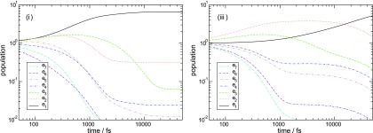
Exciton eigenstate populations calculated with the initial condition ρ_ee = 1 for models (i) and (iii) as indicated.

We next discuss how the exciton dynamics described above shows up in spectroscopic signals. The absorption spectrum, shown in Fig. 4, reflects exciton interband coherences between the ground state and the single excitons. The different types of correlations affect the line broadening (the oscillator strength is controlled by the transition dipoles which do not depend on bath). Different correlation models affect mostly the 12 200 and 12 400 cm⁻¹ regions. Interband coherences involving excitons 2–6 are thus most strongly affected by correlations. However, the exciton transitions extensively overlap and the absorption is not sensitive enough to correlations of fluctuations.

FIG. 4.

Absorption spectrum of FMO for the three models of fluctuations.

The single-exciton dynamics of Fig. 3 is directly mapped by 2D spectroscopy. Since we plot the rephasing signals, on the diagonal we solely have contributions from exciton populations during the t₂ interval.³² On the off-diagonal region the peaks belong to populations and coherences at t₂. The 2D photon echo spectra shown in Fig. 5 for the three fluctuation models at t₂ =0 are very similar on the diagonal region, but show large differences in the off-diagonal area below the diagonal. At t₂ = 0 populations of all models are identical, only spectral broadening along Ω₁ and Ω₃ axes are affected by correlations. The interference pattern of these cross-peaks reshapes the spectrum. The positive (green–yellow) peaks indicate the ESA pathways and those become very strong for correlated exponential fluctuations. This shows that correlated fluctuations are responsible for larger shifts between ESA and ESE pathways, which do not cancel.

FIG. 5.

2D spectrum of FMO calculated using the three models of fluctuations for t₂ = 0 as indicated. Regions A–F (each 50 × 50 cm⁻¹) were selected for further examination of the time t₂ dependence. This is shown in Fig. 6.

We have selected six areas of the 2D spectrum, which correspond to the most prominent peaks in the 2D spectrum, and their cross-peaks to monitor their variation with the population delay time t₂. The results are shown in Fig. 6. Diagonal peaks are A, C, and E (small oscillatory components should be ignored—they come from partial overlap with nearby cross-peaks). There is a clear difference between blue line [model (iii)] and black (and red) lines in peaks A and especially C. Population redistribution in the interval 200–1000 fs is much weaker in cut-off model for these excitons (1 and 2) in accord with Fig. 3. However, exciton dynamics in peak E, which shows higher-lying excitons, is similar. The most notable difference is the highly oscillatory cross-peak dynamics for correlated fluctuation models. Exponential correlations mostly increase the oscillation decay time of all B, D, and F peak oscillations compared to the uncorrelated fluctuation model. The cut-off correlations affect the various peaks differently: in peaks C–F the oscillations decay is similar to the uncorrelated model, but peak B shows very long-lived oscillations, which do not decay with the longest time studied (1 ps).

FIG. 6.

Time-dependent amplitudes of the A–F regions of Fig. 5 for the three fluctuation models.

VII. DISCUSSION

In this paper we presented theoretical analysis and numerical modeling of exciton dynamics for a model with correlated molecular transition energy fluctuations for the FMO complex. Fully correlated fluctuations do not affect the single-exciton density matrix evolution and, thus, the intraband coherences and populations transport. An uncorrelated model (i) allows for population transport; however, the intraband coherences are strongly damped. Partially correlated transition energy fluctuations are considered numerically. Long-lived (1 ps) coherences have been observed in several photosynthetic complexes by Engel,³³ Calhoun,¹⁶ and Collini.¹⁷ Our simulations suggest that significant component of line broadening in experiments may be attributed to correlated fluctuations in protein environment.

We considered two types of correlated fluctuations. Exponentially decaying correlations with intermolecular distance do not introduce qualitatively new features compared to the fully uncorrelated model since the FMO complex is compact (close to spherical) and the distances between neighboring chromophores do not differ significantly. The ∼30 Å correlations thus result in approximately three times reduction for the rates of exciton transport. The other model of correlated fluctuations assumes that the following chromophores 3, 4 and 5, 6 are fully correlated. This strongly affects the population transport pathways.

Correlations affect the absorption spectrum only weakly. The spectrum when all chromophores are fully correlated is similar as well (not shown). Small variations in the absorption spectrum are masked by other broadening mechanisms. However, the different patterns of correlations strongly affect the 2D spectrum, especially the cross-peak amplitudes. Most simulations of FMO 2D spectra can get quite good agreement with experiment of the diagonal peaks; however, it is very hard to match the off-diagonal cross-peaks.^13,34–38 Our simulations show that correlations shape the cross-peak region. This may be exploited to reveal the correlation pattern.

Correlated fluctuations control single-exciton population and coherence dynamics, which may be observed through the decay and oscillations of various diagonal and cross-peaks in photon echo 2D spectrum. Fully correlated fluctuations only cause interband spectral broadening, whereas uncorrelated fluctuations induce intraband coherence broadening. This is easily understood by examining how molecular energy fluctuations transform into the exciton eigenstate basis. Consider the single-exciton block of the Hamiltonian. On the diagonal we have molecular transition energies and on the off-diagonal part we have intermolecular couplings. Fully correlated fluctuations are equivalent to adding a diagonal matrix $\delta \varepsilon \mathit{I}$ (δε is the fluctuation magnitude and $\mathit{I}$ is the unit matrix). This does not affect the eigenstates, only the eigenenergies are shifted by the value δε. Thus, the single-exciton energies shift up or down: spacings of single-exciton states, which affect coherences, do not change. This modulation of exciton energies, when energy gaps are conserved, cause no intraband coherence damping. The same argument may be used to show that correlated fluctuations do not cause population transport. The transport is induced by eigenstate dynamic couplings caused by loss of correlations.

Our simulations demonstrate that a specific pattern of correlations is important for small molecular aggregates. How to measure this pattern is an open question. FMO is a pigment-protein aggregate where the chromophore surrounding is made of proteins. Proteins usually have long-range structural order (design) and have charged side-chains. These may affect chromophore transition energies through electrostatic Stark effect. The resulting fluctuations will have both long-range and short-range correlations. The fluctuation spectral density may be described by the molecular-dynamics simulations, which is the most promising tool to reveal the correlation pattern. Phenomenological models of correlations [e.g., model (ii) or (iii)] may successfully work for large molecular aggregates such as photosystem I or whole photosystem II, but may not be realistic for small molecular aggregates such as FMO.

Other mechanisms, which preserve exciton coherences, should not be ruled out. We have recently shown that a quantum transport also affects intraband single-exciton dynamics in a way that population transport is coupled with coherences and gets oscillatory components.³² Oscillatory populations translate into oscillatory diagonal peaks in the rephasing part of the 2D photon echo spectrum, which are signatures of quantum transport. Correlated energy fluctuations, on the contrary, do not lead to oscillations of exciton populations. More rigorous theory of hierarchical equations of motion developed by the groups of Tanimura and Yan include quantum transport;^39,40 however, they have not included correlated fluctuations of the bath. Quantum transport with correlated fluctuations can be described using the theory developed in Ref. 10, which explicitly includes collective bath modes.

APPENDIX: EXPRESSIONS FOR THE PHOTON ECHO SIGNAL

In this section we present closed expressions for the photon echo response function.¹⁴ There are three main contributions corresponding to a three Feynman diagrams of Fig. 1. ESA diagram denotes the excited state absorption, where during the t₂ interval the system is in the single-exciton manifold and during t₃ absorption of additional quantum induces transition into the double-exciton manifold. ESE diagram reflects the stimulated emission where the single-exciton (during t₂) emits photon. The third GSB diagram shows the system back in the ground state at t₂ interval and then the next transition (absorption) appears as bleaching. The population transport happens in ESA and ESE parts. We thus get five contributions to the response function: ESA with coherences during t₂, ESA with populations during t₂, ESE with coherences, ESE with populations, and finally GSB part. This distinction becomes possible due secular approximation for the density matrix propagation. The response function are obtained using the second-order cumulant expansion of diagonal eigenenergy fluctuations. Using the contribution labeling as in the main text, we have

$$\begin{array}{ccc}\hfill S_{AP}(t_3,t_2,t_1)& =& -i^3\sum _{e{e}^{\prime }f}{\mathit{\mu }}_{f{e}^{\prime }}{\mathit{\mu }}_{e^{\prime }f}{\mathit{\mu }}_{eg}{\mathit{\mu }}_{ge}\hfill \\ & & \times {\mathcal{G}}_{e^{\prime }{e}^{\prime },ee}\left(t_2\right)\exp \left[-i{\xi }_{f{e}^{\prime }}{t}_3-i{\xi }_{ge}{t}_1+{\varphi }_{f{e}^{\prime }e}^{\left(AP\right)}\right],\hfill \end{array}$$ (A1)

$$\begin{array}{ccc}\hfill S_{AC}(t_3,t_2,t_1)& =& -i^3\sum _{e{e}^{\prime }}^{e\ne e^{\prime }}{\mathit{\mu }}_{fe}{\mathit{\mu }}_{e^{\prime }f}{\mathit{\mu }}_{e^{\prime }g}{\mathit{\mu }}_{ge}\hfill \\ & & \times \exp \left[-i{\xi }_{fe}{t}_3-i{\xi }_{e^{\prime }e}{t}_2-i{\xi }_{ge}{t}_1+{\varphi }_{f{e}^{\prime }e}^{\left(AC\right)}\right],\hfill \end{array}$$ (A2)

$$\begin{array}{ccc}\hfill S_{EP}(t_3,t_2,t_1)& =& i^3\sum _{e{e}^{\prime }}⟨{\mathit{\mu }}_{g{e}^{\prime }}{\mathit{\mu }}_{e^{\prime }g}{\mathit{\mu }}_{eg}{\mathit{\mu }}_{ge}⟩{\mathcal{G}}_{e^{\prime }{e}^{\prime },ee}\left(t_2\right)\hfill \\ & & \times \exp \left[-i{\xi }_{e^{\prime }g}{t}_3-i{\xi }_{ge}{t}_1+{\varphi }_{e^{\prime }e}^{\left(EP\right)}\right],\hfill \end{array}$$ (A3)

$$\begin{array}{ccc}\hfill S_{EC}(t_3,t_2,t_1)& =& i^3\sum _{e{e}^{\prime }}^{e\ne e^{\prime }}{\mathit{\mu }}_{g{e}^{\prime }}{\mathit{\mu }}_{eg}{\mathit{\mu }}_{e^{\prime }g}{\mathit{\mu }}_{ge}\hfill \\ & & \times \exp \left[-i{\xi }_{e^{\prime }g}{t}_3-i{\xi }_{e^{\prime }e}{t}_2-i{\xi }_{ge}{t}_1+{\varphi }_{e^{\prime }e}^{\left(EC\right)}\right],\hfill \end{array}$$ (A4)

$$\begin{array}{ccc}\hfill S_B(t_3,t_2,t_1)& =& i^3\sum _{e{e}^{\prime }}{\mathit{\mu }}_{g{e}^{\prime }}{\mathit{\mu }}_{e^{\prime }g}{\mathit{\mu }}_{eg}{\mathit{\mu }}_{ge}\hfill \\ & & \times \exp \left[-i{\xi }_{e^{\prime }g}{t}_3-i{\xi }_{ge}{t}_1+{\varphi }_{e^{\prime }e}^{\left(B\right)}\right].\hfill \end{array}$$ (A5)

where ${\xi }_{ab}={\omega }_{ab}-i({\tau }_a^{-1}+{\tau }_b^{-1})/2$ and τ_a is a lifetime of state a. Only uncorrelated or partially correlated fluctuations should be included in dephasing functions ${\varphi }_{abc}^{\left(j\right)}$ [fully correlated part should be included via convolutions of Eqs. (42)–(49)]:

$$\begin{array}{ccc}\hfill {\varphi }_{e^{\prime }e}^{EP}(t_3,t_2,t_1)& =& {\delta }_{e^{\prime }e}{\phi }_{egeg}^{*}(t_1,t_1+t_2+t_3,t_1+t_2,0)\hfill \\ & & +(1-{\delta }_{e^{\prime }e}){\overline{\phi }}_{e^{\prime }g{e}^{\prime }e}^{*}(t_3,t_2,t_1),\hfill \end{array}$$ (A6)

$${\varphi }_{e^{\prime }e}^{EC}(t_3,t_2,t_1)={\phi }_{e^{\prime }geg}^{*}(t_1,t_1+t_2+t_3,t_1+t_2,0),$$ (A7)

$${\varphi }_{e^{\prime }e}^B(t_3,t_2,t_1)={\phi }_{e^{\prime }geg}^{*}(t_1+t_2,t_1+t_2+t_3,t_1,0),$$ (A8)

$${\varphi }_{f{e}^{\prime }e}^{AC}(t_3,t_2,t_1)={\phi }_{e^{\prime }feg}^{*}(t_1,t_1+t_2,t_1+t_2+t_3,0),$$ (A9)

$$\begin{array}{ccc}\hfill {\varphi }_{f{e}^{\prime }e}^{AP}(t_3,t_2,t_1)& =& {\delta }_{e^{\prime }e}{\phi }_{efeg}^{*}(t_1,t_1+t_2,t_1+t_2+t_3,0)\hfill \\ & & +(1-{\delta }_{e^{\prime }e}){\overline{\phi }}_{f{e}^{\prime }{e}^{\prime }e}^{*}(t_3,t_2,t_1).\hfill \end{array}$$ (A10)

These phase functions are given by

$$\begin{array}{ccc}\hfill {\phi }_{cbag}({\tau }_4,{\tau }_3,{\tau }_2,{\tau }_1)& =& -g_{cc}\left({\tau }_{43}\right)-g_{bb}\left({\tau }_{32}\right)-g_{aa}\left({\tau }_{21}\right)-g_{cb}\left({\tau }_{42}\right)\hfill \\ & & +g_{cb}\left({\tau }_{43}\right)+g_{cb}\left({\tau }_{32}\right)-g_{ca}\left({\tau }_{41}\right)\hfill \\ & & +g_{ca}\left({\tau }_{42}\right)+g_{ca}\left({\tau }_{31}\right)-g_{ca}\left({\tau }_{32}\right)\hfill \\ & & -g_{ba}\left({\tau }_{31}\right)+g_{ba}\left({\tau }_{32}\right)+g_{ba}\left({\tau }_{21}\right),\hfill \end{array}$$ (A11)

$$\begin{array}{ccc}\hfill {\overline{\phi }}_{cb{e}^{\prime }e}(t_3,t_2,t_1)& =& -g_{ee}\left(t_1\right)-g_{bb}\left(t_3\right)-g_{cc}\left(t_3\right)-g_{be}(t_1+t_2+t_3)\hfill \\ & & +g_{be}(t_1+t_2)+g_{be}(t_2+t_3)-g_{be}\left(t_2\right)\hfill \\ & & +g_{ce}(t_1+t_2+t_3)-g_{ce}(t_1+t_2)\hfill \\ & & -g_{ce}(t_2+t_3)+g_{ce}\left(t_2\right)\hfill \\ & & +g_{cb}\left(t_3\right)+g_{bc}\left(t_3\right)+2i\Im [g_{c{e}^{\prime }}(t_2+t_3)\hfill \\ & & -g_{c{e}^{\prime }}\left(t_2\right)-g_{c{e}^{\prime }}\left(t_3\right)+g_{b{e}^{\prime }}\left(t_2\right)\hfill \\ & & -g_{b{e}^{\prime }}(t_2+t_3)+g_{b{e}^{\prime }}\left(t_3\right)].\hfill \end{array}$$ (A12)

REFERENCES

- 1.Cogdell R. J., Gall A., and Köhler J., Q. Rev. Biophys. 39, 227 (2006). 10.1017/S0033583506004434 [DOI] [PubMed] [Google Scholar]
- 2.Light-Harvesting Antennas in Photosynthesis, edited by Green B. R. and Parson W. W. (Springer, New York, 2003). [Google Scholar]
- 3.Blankenship R. E., Molecular Mechanisms of Photosynthesis (Wiley-Blackwell, Oxford, 2002). [Google Scholar]
- 4.van Amerogen H., Valkunas L., and van Grondelle R., Photosynthetic Excitons (World Scientific, Singapore, 2000). [Google Scholar]
- 5.Amunts A., Drory O., and Nelson N., Nature (London) 447, 58 (2007). 10.1038/nature05687 [DOI] [PubMed] [Google Scholar]
- 6.Guskov A., Kern J., Gabdulkhakov A., Broser M., Zouni A., and Saenger W., Nat. Struct. Mol. Biol. 16, 334 (2009). 10.1038/nsmb.1559 [DOI] [PubMed] [Google Scholar]
- 7.Adolphs J. and Renger T., Biophys. J. 91, 2778 (2006). 10.1529/biophysj.105.079483 [DOI] [PMC free article] [PubMed] [Google Scholar]
- 8.Rebentrost P., Mohseni M., and Guzik A. A., J. Phys. Chem. B 113, 9942 (2009). 10.1021/jp901724d [DOI] [PubMed] [Google Scholar]
- 9.May V. and Kühn O., Charge and Energy Transfer Dynamics in Molecular Systems (Wiley-VCH, Weinheim, 2011). [Google Scholar]
- 10.Chernyak V. and Mukamel S., J. Chem. Phys. 105, 4565 (1996). 10.1063/1.472302 [DOI] [Google Scholar]
- 11.Mukamel S., Annu. Rev. Phys. Chem. 51, 691 (2000). 10.1146/annurev.physchem.51.1.691 [DOI] [PubMed] [Google Scholar]
- 12.Jonas D. M., Annu. Rev. Phys. Chem. 54, 425 (2003). 10.1146/annurev.physchem.54.011002.103907 [DOI] [PubMed] [Google Scholar]
- 13.Cho M., Chem. Rev. 108, 1331 (2008). 10.1021/cr078377b [DOI] [PubMed] [Google Scholar]
- 14.Abramavicius D., Palmieri B., Voronine D. V., Šanda F., and Mukamel S., Chem. Rev. 109, 2350 (2009). 10.1021/cr800268n [DOI] [PMC free article] [PubMed] [Google Scholar]
- 15.Panitchayangkoon G., Hayes D., Fransted K. A., Caram J., Harel E., Wen J., Blankenship R., and Engel G., Proc. Natl. Acad. Sci. U.S.A. 107, 12766 (2010). 10.1073/pnas.1005484107 [DOI] [PMC free article] [PubMed] [Google Scholar]
- 16.Calhoun T. R., Ginsberg N. S., Schlau-Cohen G. S., Cheng Y.-C., Ballottari M., Bassi R., and Fleming G. R., J. Phys. Chem. B 113, 16291 (2009). 10.1021/jp908300c [DOI] [PubMed] [Google Scholar]
- 17.Collini E., Wong C. Y., Wilk K. E., Curmi P. M.G., Brumer P., and Scholes G. D., Nature (London) 463, 644 (2010). 10.1038/nature08811 [DOI] [PubMed] [Google Scholar]
- 18.Nemeth A., Milota F., Mancal T., Lukes V., Hauer J., Kauffmann H. F., and Sperling J., J. Chem. Phys. 132, 184514 (2010). 10.1063/1.3404404 [DOI] [Google Scholar]
- 19.Lee H., Cheng Y.-C., and Fleming G., Science 316, 1462 (2007). 10.1126/science.1142188 [DOI] [PubMed] [Google Scholar]
- 20.Milder M. T.W., Brüggemann B., van Grondelle R., and Herek J. L., Photosynth. Res. 104, 257 (2010). 10.1007/s11120-010-9540-1 [DOI] [PMC free article] [PubMed] [Google Scholar]
- 21.Renger T., May V., and Kühn O., Phys. Rep. 343, 137 (2001). 10.1016/S0370-1573(00)00078-8 [DOI] [Google Scholar]
- 22.Mukamel S., Principles of Nonlinear Optical Spectroscopy (Oxford University Press, New York, 1995). [Google Scholar]
- 23.Chernyak V., Minami T., and Mukamel S., J. Phys. Chem. 112, 7953 (2000). 10.1063/1.481396 [DOI] [Google Scholar]
- 24.Zhang W. M., Meier T., Chernyak V., and Mukamel S., J. Chem. Phys. 108, 7763 (1998). 10.1063/1.476212 [DOI] [Google Scholar]
- 25.Mukamel S. and Loring R. F., J. Opt. Soc. Am. B 3, 595 (1986). 10.1364/JOSAB.3.000595 [DOI] [Google Scholar]
- 26.Abramavicius D. and Mukamel S., J. Chem. Phys. 124, 034113 (2006). 10.1063/1.2104527 [DOI] [PubMed] [Google Scholar]
- 27.Mukamel S., Annu. Rev. Phys. Chem. 51, 691 (2000). 10.1146/annurev.physchem.51.1.691 [DOI] [PubMed] [Google Scholar]
- 28.Mukamel S., Abramavicius D., Yang L., Zhuang W., Schweigert I. V., and Voronine D., Acc. Chem. Res. 42, 553 (2009). 10.1021/ar800258z [DOI] [PMC free article] [PubMed] [Google Scholar]
- 29.Hahn E. L., Phys. Rev. 80, 580 (1950). 10.1103/PhysRev.80.580 [DOI] [Google Scholar]
- 30.Read E. L., Engel G. S., Calhoun T. R., Mančal T., Ahn T. K., Blankenship R. E., and Fleming G. R., Proc. Nat. Acad. Sci. U.S.A. 104, 14203 (2007). 10.1073/pnas.0701201104 [DOI] [PMC free article] [PubMed] [Google Scholar]
- 31.Brixner T., Stenger J., Vaswani H. M., Cho M., Blankenship R. E., and Fleming G. R., Nature (London) 434, 625 (2005). 10.1038/nature03429 [DOI] [PubMed] [Google Scholar]
- 32.Abramavicius D. and Mukamel S., J. Chem. Phys. 133, 064510 (2010). 10.1063/1.3458824 [DOI] [PubMed] [Google Scholar]
- 33.Engel G. S., Calhoun T. R., Read E. L., Ahn T. K., Mančal T., Cheng Y. C., Blankenship R. E., and Fleming G. R., Nature (London) 446, 782 (2007). 10.1038/nature05678 [DOI] [PubMed] [Google Scholar]
- 34.Sharp L. Z., Egorova D., and Domcke W., J. Chem. Phys. 132, 014501 (2010). 10.1063/1.3268705 [DOI] [PubMed] [Google Scholar]
- 35.Brüggemann B., Kjellberg P., and Pullerits T., Chem. Phys. Lett. 444, 192 (2007). 10.1016/j.cplett.2007.07.002 [DOI] [Google Scholar]
- 36.Voronine D. V., Abramavicius D., and Mukamel S., Biophys. J. 95, 4896 (2008). 10.1529/biophysj.108.134387 [DOI] [PMC free article] [PubMed] [Google Scholar]
- 37.Abramavicius D., Palmieri B., and Mukamel S., Chem. Phys. 357, 79 (2009). 10.1016/j.chemphys.2008.10.010 [DOI] [PMC free article] [PubMed] [Google Scholar]
- 38.Cho M., Vaswani H. M., Brixner T., Stenger J., and Fleming G. R., J. Phys. Chem. B 109, 10542 (2005). 10.1021/jp050788d [DOI] [PubMed] [Google Scholar]
- 39.Tanimura Y., J. Phys. Soc. Jpn. 75, 082001 (2006). 10.1143/JPSJ.75.082001 [DOI] [Google Scholar]
- 40.Xu R.-X., Cui P., Li X.-Q., Mo Y., and Yan Y.-J., J. Chem. Phys. 122, 041103 (2005). 10.1063/1.1850899 [DOI] [Google Scholar]