Abstract
Purpose:
To investigate a novel locally adaptive projection space denoising algorithm for low-dose CT data.
Methods:
The denoising algorithm is based on bilateral filtering, which smooths values using a weighted average in a local neighborhood, with weights determined according to both spatial proximity and intensity similarity between the center pixel and the neighboring pixels. This filtering is locally adaptive and can preserve important edge information in the sinogram, thus maintaining high spatial resolution. A CT noise model that takes into account the bowtie filter and patient-specific automatic exposure control effects is also incorporated into the denoising process. The authors evaluated the noise-resolution properties of bilateral filtering incorporating such a CT noise model in phantom studies and preliminary patient studies with contrast-enhanced abdominal CT exams.
Results:
On a thin wire phantom, the noise-resolution properties were significantly improved with the denoising algorithm compared to commercial reconstruction kernels. The noise-resolution properties on low-dose (40 mA s) data after denoising approximated those of conventional reconstructions at twice the dose level. A separate contrast plate phantom showed improved depiction of low-contrast plates with the denoising algorithm over conventional reconstructions when noise levels were matched. Similar improvement in noise-resolution properties was found on CT colonography data and on five abdominal low-energy (80 kV) CT exams. In each abdominal case, a board-certified subspecialized radiologist rated the denoised 80 kV images markedly superior in image quality compared to the commercially available reconstructions, and denoising improved the image quality to the point where the 80 kV images alone were considered to be of diagnostic quality.
Conclusions:
The results demonstrate that bilateral filtering incorporating a CT noise model can achieve a significantly better noise-resolution trade-off than a series of commercial reconstruction kernels. This improvement in noise-resolution properties can be used for improving image quality in CT and can be translated into substantial dose reduction.
Keywords: CT, radiation dose, noise reduction, bilateral filtering, denoising
I. INTRODUCTION
Radiation exposure and the associated risk of cancer for patients receiving CT examinations have been an increasing concern in recent years.1,2 It is critically important to reduce the radiation dose level in CT examinations. However, dose reduction generally leads to an increased level of noise in the measured projection data and the subsequent reconstructed images, thus degrading the diagnostic value of the CT examination.
Many techniques have been developed for controlling noise in CT, operating on either the raw projection measurement, the log-transformed sinogram, during image reconstruction, or on images after reconstruction.3–10 In conventional shift-invariant filtration applied during image reconstruction, the suppression of the high-frequency component in the sinogram is performed with a simple assumption that all the measurements are equally reliable, which may result in severe degradation of spatial resolution.3–8 More sophisticated methods have been developed to adaptively smooth the data by taking into account the local statistics in the measurements. Hsieh used an adaptive trimmed mean filter to smooth the data with the filter strength changing with the detected signal.4 The method of Kachelriess et al. was similar except that it was generalized to include both the 2D detector array and the angular dimension and used a direct threshold on projection data as opposed to a more accurate noise model.5 Some of these methods are currently implemented on clinical scanners mainly to suppress the streaking artifacts caused by x-ray photon starvation. Many other approaches have also been proposed to incorporate more explicit statistical models and to iteratively restore the log-transformed data by optimizing a penalized weighted least-squares or likelihood objective function, in some cases by relating the sinogram value to its variance, thus empirically characterizing the noise of the sinogram value after processing (beam-hardening correction, calibration, etc.).6,7 Other approaches model CT noise in a more complete way, including compound Poisson, off-focal, cross-talk, and other effects.8,9 Iterative reconstruction methods can achieve significant denoising but at the expense of very long computation times.10 Techniques based entirely on image space have also been described, taking advantage of the image structure to smooth noise while preserving edges but suffering from the complicated properties of noise in image space in CT.11–13
In this work, we investigated a locally adaptive method for noise control in CT. This method is based on bilateral filtering,14 which smooths the sinogram by using a weighted average in a local neighborhood, with the weights determined according to both the spatial proximity and intensity similarity between the center pixel and the neighboring pixels. This filtering is locally adaptive and can preserve important edge information in the sinogram, thus maintaining high spatial resolution. It is closely related to anisotropic diffusion15 but is much faster. Furthermore, since it originated from the statistical framework of maximum a posteriori (MAP) estimation,16 a CT noise model can be incorporated, which is critical for effective noise reduction in low-dose CT. Note that Demirkaya17 proposed anisotropic diffusion filtering in projection space, but with a crude noise model and only showing results on a synthetically corrupted Shepp–Logan phantom.
While some denoising or sinogram restoration methods have been developed to smooth the projection data by taking explicit statistical models into account,6–9 the proposed approach is noniterative and is easier to implement in practice. Compared to adaptive filters developed to suppress the streaking artifacts caused by the photon starvation along some directions,4,5 the proposed approach aims to perform noise reduction in the full projection dataset while preserving structural detail.
This paper is organized as follows. In Sec. II, we introduce bilateral filtering and its application to CT data denoising, describe the effects of the bowtie filter and automatic exposure control and their inclusion in the CT noise model, and present the evaluation methodology. In Sec. III, the evaluation results are presented and discussed. Finally, we present conclusions in Sec. IV.
II. METHODS
II.A. Bilateral filtering
Bilateral filtering was originally proposed by Tomasi and Manduchi as a noniterative and locally adaptive method for removing additive noise from images while preserving edge information.14 In addition to its intuitive appeal, the bilateral filter also has strong origins in MAP estimation.16
Suppose is a stationary Gaussian process with a mean of
| (1) |
where is a white Gaussian noise added to the original image . We use a bold letter and the corresponding normal letter to denote a stochastic process and its mean, respectively. To restore the original image from the noise contaminated image , we consider minimizing the energy functional
| (2) |
where calculates a weight according to the spatial distance between the center pixel and a neighboring pixel and the second penalty factor calculates a weight according to the pixel value difference between the center pixel and a neighboring pixel. Additionally, is the index of a neighborhood pixel inside a region of centered on pixel , and the outer sum is taken over all pixels in image . Minimizing this functional encourages local groups of pixels to be of similar intensity, resulting in an image with overall piecewise homogeneity. Moreover, in the restricted case where only immediate neighbors are investigated and the spatial penalty function is taken as the identity operator, Eq. (1) is the same functional that is minimized by the classical anisotropic diffusion process for image denoising.15
While there are many possibilities for choosing the penalty functions and , the most common assignments are the Gaussian penalties given by
| (3) |
| (4) |
where parameters and σ can be used for controlling the spatial and intensity range of the weighting. Following Elad,16 the bilateral filter arises as the first iteration of a Jacobi process minimizing Eq. (2) and is formally defined by the weighted averaging of a given image pixel , namely,
| (5) |
where and are the differentials of and and, after certain factors cancel,
| (6) |
which are again Gaussian. Under the specification in Eqs. (3) and (4) with Gaussian weighting functions, the bilateral filter is identical to the Nadaraya–Watson estimator commonly employed in nonparametric kernel regression. While repeated iterations are possible to further minimize the energy functional (2), in practice, only a single pass of the bilateral filter is generally needed to obtain substantial denoising results. Furthermore, a separable approximation of the bilateral filter, as proposed by Pham and van Vliet,18 is available and allows for a dramatic increase in computational performance with little to no degradation in efficacy. This approximation consists simply of running a one-dimensional filter in one direction first, then applying the filter to the results of this step in the other direction, analogous to the way FFTs are usually calculated. For all applications in this work, the separable approximation is employed.
II.B. CT noise model
Denoising with bilateral filtering can be directly applied in image space after reconstruction, and indeed the sharper edges there are well suited to techniques like bilateral filtering, but the noise model in image space is very complex due to the data preprocessing and image reconstruction. In contrast, noise in projection space is relatively easier to model under certain simplified assumptions. In this study, we will focus only on the application of bilateral filtering to projection space denoising.
Noise in CT images originates from data noise in the projection measurement, which has two principal sources: Quantum noise and electronic noise. The electronic noise is the result of electronic fluctuation in the detector photodiode and other electronic components. The quantum noise is due to the limited number of photons collected by the detector. Although a current CT detector is not a photon-counting element but an energy integrator that generates a signal proportional to the total energy deposited in the detector, a photon-counting model is still a good approximation and is widely used for characterizing noise properties of the CT data.10,19,20 More accurate noise models have been investigated, such as the compound Poisson model that takes into account the polychromatic x-ray beam and energy integration.21 As explained therein, the actual residual error introduced by a photon-counting model is only a few percent for typical photon flux level in clinical CT protocols. As also indicated in that work, the impact from the bowtie filter and tube current modulation on noise characteristics of CT data is even more significant. Therefore, for simplicity, we use a photon-counting model and will consider the effect of the bowtie filter and tube current modulation in this work.
For a given attenuating path in the imaged subject, denote the incident and the penetrated photon numbers as and , respectively, where α and denote the index of detector bins along the radial and longitudinal directions, and λ the index of projection angle. In the presence of noise, the measured data should be considered as a stochastic process. Ideally, the line integral along the attenuating path is given by . Herein, we neglect the detector index (α, ν, λ) in all the variables unless explicitly indicated.
We assume that is a deterministic constant and is Poisson distributed with mean . We also neglect the electronic noise and assume that the data collected on each detector bin are uncorrelated. The number of input photons must now be estimated as a function of α, ν, and λ.
II.C. Incorporation of the effect of x-ray beam bowtie filter
The incident number of photons varies for each projection angle due to the use of the automatic exposure control (AEC) technique22 and is also nonuniform across the radiation field of the x-ray beam mainly due to the use of the beam-shaping bowtie filter.23 To accurately quantify the noise properties in the projection data and preserve the noise pattern in the denoised image, these effects must be taken into consideration. This task can simply be accomplished by expressing the incident number of photons as a function of detector bin index α and based on the estimation of the nonuniformity across the x-ray radiation field and a function of projection angle λ based on the estimation of the tube current modulation.
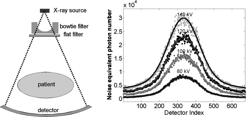
As shown in Fig. 1 (left), a bowtie filter is usually used in the x-ray beam. Because the cross section of most patients is ovally or circularly shaped, the attenuation in the peripheral region is much less than that in central region. The purpose of the bowtie filter is to reduce the incident x-ray intensity in the peripheral region so that the radiation dose to the patient, especially the skin dose, can be minimized. As a consequence, the x-ray intensity incident to the patient is highly nonuniform across the fan beam, which affects the noise properties in the measured CT data. We empirically determine the effect of the bowtie filter by measuring the variance of the transmission from an air scan. The inverse of the variance is a number that can be used to estimate the incident x-ray intensity across the x-ray beam.21 Figure 1 (right) displays an example of the noise-equivalent incident quanta number on a single detector row across the x-ray beam obtained for different tube potentials (kV). By fitting the variance with a third- or fourth-order Gaussian equation, four calibration curves of the incident x-ray intensity for the kVs at 80, 100, 120, and 140 are obtained. Such calibration curves may be different, depending on the configuration of the detector collimation.
FIG. 1.
Effect of x-ray beam bowtie filter. Left: Illustration of the bowtie filter in the x-ray beam to reduce the incident x-ray intensity in the peripheral region of the x-ray fan-beam. Right: An example of noise-equivalent number of x-ray quanta curves for 140, 120, 100, and 80 kV that can be used for characterizing the effect of the nonuniform photon intensity caused by the bowtie filter.
II.D. Incorporation of AEC
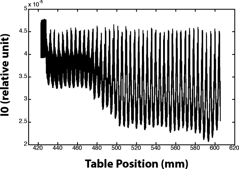
AEC is widely used for dose reduction in abdominal CT. Figure 2 shows one example of tube current modulation from a CT scanner. The curve represents the reference signals of the tube as a function of the table position, which corresponds to a certain tube angle. The reference signal is proportional to the tube current used for that table position and projection angle. As can be seen, the tube current oscillates during the gantry rotation in order to adapt to the attenuation level of the patient along different orientations. This automatic tube current modulation leads to a continuous change in the incident x-ray intensity, which will also affect the noise characteristics of the CT data. We incorporate this effect by extracting the reference signal from each projection frame and then estimating the corresponding reference x-ray intensity. The calibration curves determined from the bowtie filter are used for this estimation.
FIG. 2.
Effect of AEC. Displayed is an example of tube current modulation from an abdominal CT exam. The curve represents the reference signals on the detector as a function of table position. The reference signal is proportional to the tube current used for that table position and projection angle. The tube current oscillates as the table translates to adapt to the different attenuation levels of the patient along different projection angles.
II.E. Sinogram smoothing with bilateral filtering
To incorporate the noise model in bilateral filtering, we first convert the measured sinogram to a dataset representing a map of detected number of photons, which is simply expressed as
| (7) |
Practically, the x-ray photons emitting from the tube are polychromatic. The total number of incident photons before the attenuation can be estimated as the noise-equivalent photon number, as detailed above. The Anscombe transform24 is a standard statistical tool to convert Poisson distributed data to data with an approximately normal distribution with a constant variance,
| (8) |
This transformation is considered valid when the mean value of the Poisson data is greater than 20. The minimum flux levels in CT data are at least several hundreds in all the datasets we have tested thus far. Here we also ignore the small constant additive factor of (negligible at these count numbers, but easily included if desired) and the multiplicative factor of 2, and simply take the square root of the photon number to generate the dataset which is subsequently used for denoising, with a constant standard deviation of . The square-root-transformed data are given by
| (9) |
Equation (5) can be applied on to obtain the denoised dataset . The steps are then reversed to convert back to the log-transformed sinogram, which can be used for regular image reconstruction.
II.F. Evaluation of noise and resolution properties
We performed phantom studies to evaluate the noise-resolution properties of bilateral filtering with CT noise modeling. These studies were performed on a dual-source CT scanner (Somatom Definition, Siemens Medical Solutions, Forchheim, Germany). A phantom with a small acrylic cylinder and a thin wire that is typically used for quality control on Siemens scanners was scanned with the following parameters: 120 kVp, 0.5 s rotation time, detector collimation, 672 × 32 detector matrix size, helical pitch of 1.0, and mA s values of 40 and 80. The images were reconstructed using a series of kernels available on the scanner with a slice thickness of 1 mm and an FOV size of 50 mm. The raw data were downloaded from the scanner and denoised with bilateral filtering. The Gaussian filter with a given spatial standard deviation in Eq. (3) was approximated to a given filter length , and we found it useful empirically to lock the ratio of to as . The denoising parameters were filter length (corresponding to and evaluated from −2 to 2) and σ = 0.7, 1, 1.4, 1.8, 2.2, and 2.8. We also explored different values of and found, as expected, that larger filters gave lower noise but lower resolution. For space reasons, we only discuss results with fixed at 5, again determined empirically. The denoised data were uploaded to the scanner and reconstructed with both the B70f and B40f kernels (the B70f kernel is an extremely sharp but noisy kernel, while the B40f is slightly sharper and noisier than is used at some institutions, but it is employed in our clinical practice for routine body CT). The modulation transfer function (MTF) on each image, either directly reconstructed on the scanner or after bilateral filter denoising, was calculated using a method similar to that in Ref. 25. The noise level at a small region of interest (ROI) 15 mm away from the wire was also measured.
A second phantom consisted of a stadium-shaped water tank (lateral width of 30 cm, height of 22.5 cm). Eight thin plates with different contrast levels (120 HU: 2; 70 HU: 3; 40 HU: 3) were placed in the central region of the water tank to allow visualization of these lower contrast materials. The scanning parameters were detector collimation 64 × 0.6 with a -flying focal spot, 120 quality reference mA s, rotation time of 0.5 s (the term “quality reference mA s” is used in the automatic exposure control software in Siemens scanners to prescribe mA s. Its value equals the effective mA s used for a standard patient size). The images were reconstructed with commercial kernels at B45, B40, B30, B20, and B10 with a slice thickness of 0.6 mm. The raw data were denoised with and σ = 1 and reconstructed with various kernels.
II.G. Evaluation in CT colonography
We performed a preliminary study to evaluate the noise-resolution properties of bilateral filtering. The tested CT raw data were obtained from a patient study undergoing a noncathartic CT colonography. The patient was scanned on the dual-source CT system with the following scanning parameters: 120 kVp, 100 quality reference mA s, 0.5 s rotation time, detector collimation, and a helical pitch of 1.4. The volume CT dose index is 7 mGy. The images were reconstructed on the scanner with a slice thickness of 1 mm and several reconstruction kernels (B10f, B20f, B30f, and B40f) that represent a trade-off between noise and resolution. The raw data were downloaded from the CT scanner and processed with bilateral filtering with different parameter settings. The smoothed data were subsequently reloaded on the scanner and reconstructed with a B40f kernel, and the noise and resolution properties were analyzed.
II.H. Evaluation in CT enterography
We applied bilateral filtering to five abdominal CT exams performed on the dual-source scanner. Each exam was scanned in a dual-energy mode with one tube operated at 140 kV and the other at 80 kV, with one-half or less of the power distributed to the 80 kV tube. The 80 kV data is acquired at 425 quality reference mA s. Two sets of images (low and high energy) were generated from each dual-energy scan. Besides the dual-energy processing that is used to provide material-specific information,26–28 the dual-energy images are mixed together in a linear fashion to form a single set of images, which serves a similar purpose as the images from a conventional single-energy scan at 120 kV.
The 80 kV images obtained from a dual-energy scan have enhanced iodine signal compared to 140 kV (the iodine signal is approximately doubled). However, they are often subject to increased noise contamination due to the higher attenuation of the low-energy x rays. Low-energy images alone are often insufficient for diagnostic purposes despite the improved contrast enhancement. We applied bilateral filtering (, σ = 1), followed by B40f reconstruction to the 80 kV images and compared these images to B40f and B20f reconstruction alone.
III. RESULTS
III.A. Noise-resolution properties
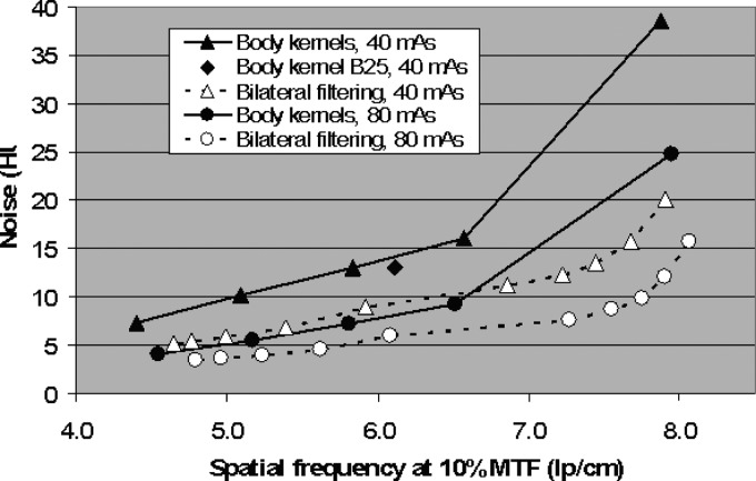
Figure 3 compares the noise-resolution properties of bilateral filtering with the body kernels available on the scanner on the thin wire phantom. The noise was represented by the standard deviation (HU) in a small ROI 15 mm away from the thin wire in the phantom. The spatial resolution was represented by the spatial frequency at 10% of the maximum value on the MTF curve. The solid curve linking the solid triangles (▲) was obtained from the image scanned with 40 mA s and reconstructed with kernels of B10f, B20f, B30f, B40f, and B50f (from left to right). As can be seen, these body kernels represent a trade-off between noise level and spatial resolution. With a smoother kernel, the noise level on the image is lower, while the spatial resolution is also lower. The solid diamond symbol (◆) was from the same scan and represents a special body kernel B25f, which involves a two-dimensional adaptive filter implemented in the image domain. It has a slightly better noise-resolution trade-off than B30 kernel. The dashed curve linking the open triangles (△) represents the noise-resolution results obtained from images after applying bilateral filtering to the 40 mA s scan data with ten different smoothing parameters. From left to right, the first five points were reconstructed with the B40f kernel, with fixed at 5, and σ = 2.2, 1.8, 1.4, 1.0, 0.7, respectively; the second five points were reconstructed with a sharper B70f kernel, with fixed at 5, σ = 2.8, 2.2, 1.8, 1.4, and 1.0, respectively. The solid curve linking the solid circles (●) was obtained from the image scanned with 80 mA s and reconstructed with kernels of B10f, B20f, B30f, B40f, and B50f (from left to right). The dashed curve linking the open circles (○) represents the noise-resolution results obtained from images after applying bilateral filtering to the 80 mA s scan data with the same ten smoothing parameters as above.
FIG. 3.
Noise-resolution properties of bilateral filtering and body kernels. Noise is expressed as the standard deviation (HU) in a small ROI close to the thin wire. The spatial resolution was quantified as the spatial frequency at 10% of the maximum value on the MTF curve. The solid curve linking the solid triangles (▲) was obtained from the image scanned with 40 mA s and reconstructed with kernels of B10f, B20f, B30f, B40f, and B50f (from left to right). The solid diamond symbol (◆) was from the same scan and represents a special body kernel B25f. The dashed curve linking the open triangles (△) represents the noise-resolution results obtained from images after applying bilateral filtering to the 40 mA s scan data with ten different smoothing parameters. From left to right, the first five points were reconstructed with the B40f kernel, with fixed at 5, and σ = 2.2, 1.8, 1.4, 1.0, 0.7, respectively; the second five points were reconstructed with a sharper B70f kernel, with fixed at 5, and σ = 2.8, 2.2, 1.8, 1.4, and 1.0, respectively. The solid curve linking the solid circles (●) was obtained from the image scanned with 80 mA s and reconstructed with kernels of B10f, B20f, B30f, B40f, and B50f (from left to right). The dashed curve linking the open circles (○) represents the noise-resolution results obtained from images after applying bilateral filtering to the 80 mA s scan data with the same ten smoothing parameters as above. The noise-resolution results on the 40 mA s data after bilateral filtering approach or exceed the noise-resolution properties of the 80 mA s data, and filtering is effective on the 80 mA s data as well as on the 40 mA s data.
One can see that a much better noise-resolution trade-off is achieved by bilateral filtering than by the body kernels alone on the 40 mA s, with noise-resolution properties approaching or exceeding the conventionally reconstructed 80 mA s data (with twice the radiation dose). For example, for a given noise level of 16 HU on the 40 mA s data, bilateral filtering (, σ = 1.4, B70f recon) yields a spatial resolution of 7.7 lp/cm at 10% MTF, much higher than does the B40f kernel without filtering (6.6 lp/cm). This is also higher resolution than the 80 mA s data reconstructed at this noise level. Conversely, at a given resolution, bilateral filtering offers much lower noise levels—e.g., the B30f kernel alone yields a noise level of 13 HU at a resolution of 5.9 lp/cm, while bilateral filtering (, σ ∼ 0.7, B40f recon) would give a noise level of 8 HU at this resolution, very close to what is achieved with twice the radiation dose. The noise-resolution results on the 40 mA s data after bilateral filtering approach or exceed the noise-resolution properties of the unfiltered 80 mA s data. A similar improvement in the noise-resolution trade-off is obtained by filtering the 80 mA s data.
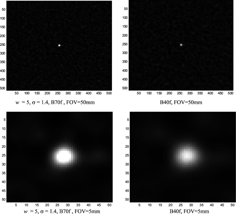
To visually demonstrate the improvement of spatial resolution, the point spread functions (PSFs) for the wire images obtained with bilateral filtering (, σ = 1.4, B70f recon) and the unfiltered B40f reconstruction are shown in Fig. 4. Both images have a similar noise level of 16 HU, but the bilateral filtered image has a sharper appearance indicated by a sharper wire shape as well as a sharper noise texture.
FIG. 4.
PSF of the wire images obtained with bilateral filtering (, σ = 1.4) with the B70f kernel (left) and the B40f kernel without filtering (right) displayed in an large FOV of 50 mm (top row) and a small FOV of 5 mm (bottom row). The images have the same noise level at 16 HU, while the image with bilateral filtering has a much sharper appearance indicated by a sharper wire shape as well as a sharper noise texture.
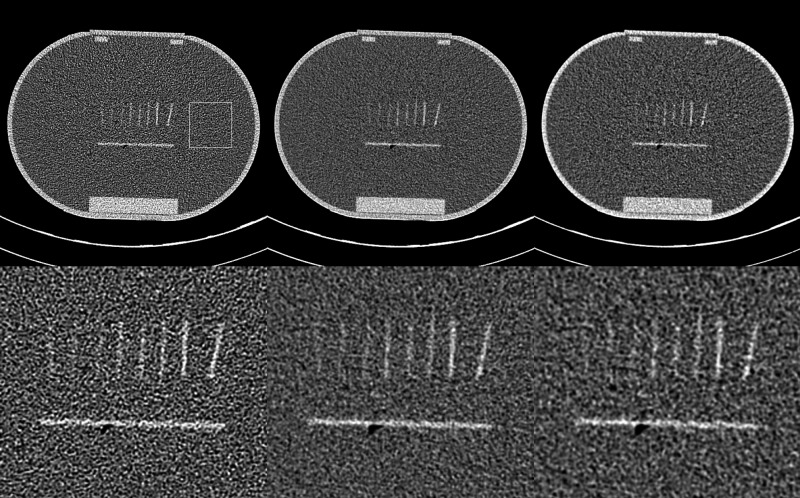
Figure 5 shows the images for the stadium-shaped phantom and blowups of the central region containing the contrast plates after B45 reconstruction (left column), bilateral filtering followed by B45 reconstruction (center), and B20 reconstruction (right). The standard deviations inside the ROI are 49.1, 31.9, and 32.9 HU, respectively. Despite the approximately matched noise levels, the lower contrast plates are, in our opinion, better visualized in the denoised image than in the B20f image.
FIG. 5.
The images for the stadium-shaped phantom after B45 reconstruction (top left), bilateral filtering followed by B45 reconstruction (top center), and B20 reconstruction (top right). The bottom row shows zoomed versions of the central region of the images. The standard deviations inside the ROI are 49.1, 31.9, and 32.9 HU, respectively. The lower contrast plates are, in our opinion, better visualized with the denoised image than with the B20f image.
III.B. Evaluation of noise-resolution properties in CT colonography
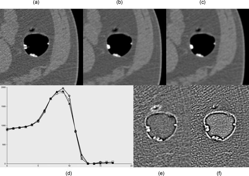
Figure 6(a) shows a slice of the noncathartic CT colonography data containing barium-tagged stool reconstructed with a standard B40f reconstruction kernel (a), with the same kernel after bilateral filtering (b) with , σ = 1.1, (c) and with the unfiltered B10f kernel. Images (b) and (c) have similar noise levels in an ROI in the lumen (14.5 and 14.7, respectively). Profiles along the stool-air boundary (d) show that the denoised B40f image has a sharper stool-air transition than the B10f, while difference images (e) and (f) show that the denoised B40f is sharper and has smaller differences from the original.
FIG. 6.
Images of the colon containing labeled stool (a) with standard B40f reconstruction kernel and a line profile across stool-air interface, (b) with B40f reconstruction after projection space bilateral filtering with , σ = 1.1, and (c) reconstructed with the unfiltered B10f kernel. (d) A profile along the line indicated in (a), showing the values (units of HU + 1024) for the B40f (○), B40f with denoising (◻), and B10f (▲). (e) Difference image between B40f and B40f with denoising reconstructions. (f) Difference image between B40f and B10f reconstructions. The difference images are at the same window and level settings.
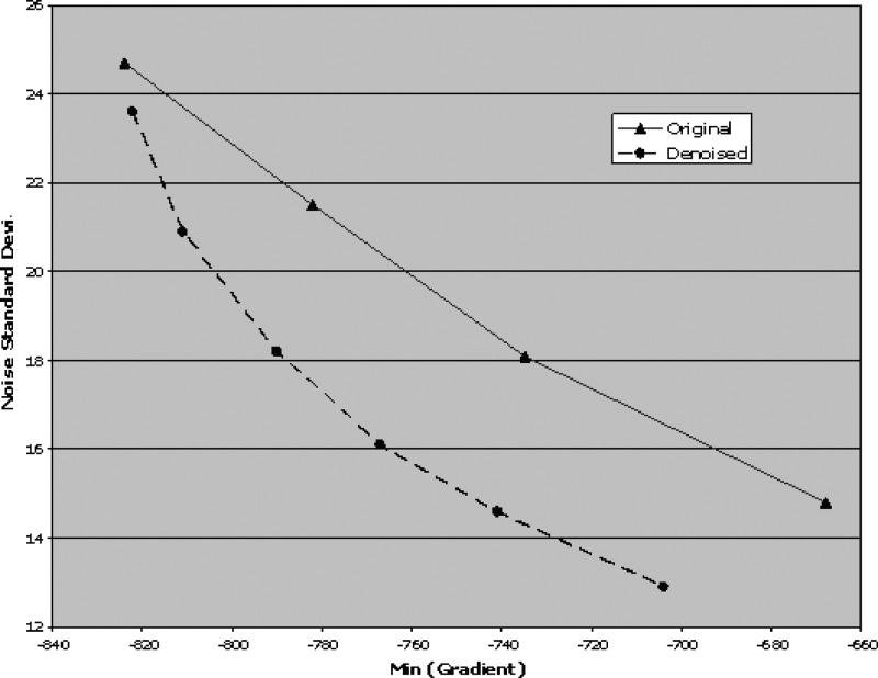
To quantitatively evaluate the resolution property of each reconstruction, we used the profile across the boundary between the labeled stool and air shown in Fig. 6(a). The gradient of the profile was calculated and the maximum negative gradient value was used for comparing the spatial resolution since it represents the sharpness of the boundary. The noise in a nearby air region (inside the lumen) was also measured for each reconstruction. Figure 7 displays the plot of noise level versus spatial resolution (represented by the maximum negative gradient value) for various reconstruction kernels and for bilateral filtering with and different σ settings, followed by a B40f reconstruction. It can be seen that bilateral filtering can reduce noise with much less effect on spatial resolution than the commercial kernels. When followed with a B40f reconstruction, for example, bilateral filtering with σ of 0.5 can achieve a lower noise level than an unfiltered B30f reconstruction, but with better resolution, while filtering with σ of 0.7 reduces noise to the level of the unfiltered B20f reconstruction with resolution still slightly better than an unfiltered B30f reconstruction. Bilateral filtering with σ of 1.1 gives slightly lower noise than the unfiltered B10f reconstruction but with significantly better resolution (these are the images shown in Fig. 6).
FIG. 7.
Standard deviation of noise in air ROI vs largest negative gradient in profile in Fig. 6(a) calculated for different reconstruction kernels and for different levels of bilateral filtering followed by standard B40f reconstruction. The solid curve linking the solid triangles (▲) was calculated from images reconstructed with kernels of B40f, B30f, B20f, and B10f (from left to right; note that sharper edges are to the left). The dashed curve linking the circles (●) was calculated from images reconstructed with the B40f kernel after denoising with and σ = 0.3, 0.5, 0.7, 0.9, 1.1, and 1.5, respectively.
III.C. Evaluation of noise-resolution properties in CT enterography
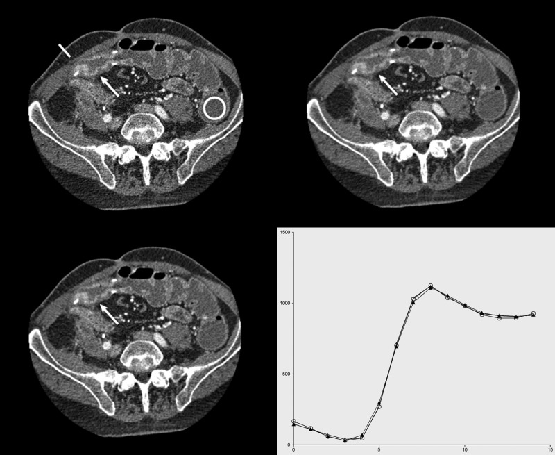
Figure 8 displays contrast-enhanced images obtained from an 80 kV CT enterography exam. The top left image was reconstructed with kernel B40f. The top right image was reconstructed with the same kernel after bilateral filtering (, σ = 1). The bottom left image represents the B20f reconstruction. The noise levels in the ROI denoted by the circle are 39.1, 25.6, and 25.9, respectively. The profile at the bottom right shows that the denoised B40f is slightly sharper than the B20f despite the similar and slightly lower noise level. The visualization of the mural stratification and delination of the inner and outer boundaries of the neoterminal ileum (arrow) has been improved by bilateral filtering, and the denoised B40f was preferred by a radiologist for diagnosis. Similar results were obtained in CT datasets visualizing the bowel , pancreas , and liver . In each case, a board-certified subspecialized radiologist rated the denoised 80 kV images markedly superior in image quality compared to the 80 kV images reconstructed with a commercially available kernel. In cases, denoising improved image quality to the point where the 80 kV images alone were considered to be of diagnostic quality (currently the mixed images, with twice the radiation dose, are used for this purpose).
FIG. 8.
Contrast-enhanced low-energy images obtained from a dual-energy CT enterography exam. Top left: The image reconstructed from the 80 kV scan with kernel B40f. The line represents the profile location and the circle represents the ROI for noise measurements. Top right: Image after bilateral filtering and reconstruction (, σ = 1, B40f). Radiologists preferred the visualization of the mural stratification in the neoterminal ileum (arrow) in the denoised image. Bottom left: Image with B20f reconstruction. The noise levels in the ROI denoted by the circle were 39.1, 25.6, and 25.9, respectively. Bottom right: Profiles across the line in the upper left showing the values for the B40f (○), B40f with denoising (+), and B20f (▲) reconstructions.
IV. CONCLUSIONS
We investigated a noniterative approach to reducing noise in CT using locally adaptive bilateral sinogram filtering with a CT noise model that included the effects of the bowtie filter and automatic exposure control. This filtering can be implemented very simply and more efficiently than many existing sinogram denoising methods. We evaluated the resolution-noise properties of bilateral filtering with CT noise modeling with phantom studies and preliminary patient studies. The results demonstrate that it can achieve a better noise-resolution trade-off than the commonly used commercial reconstruction kernels. Such noise reduction should be translatable to improvements in image quality and/or substantial dose reduction in CT.
We expect this method to have difficulty with small, low-contrast objects and with subtle texture with intensity near the noise level, but this is true for most other denoising algorithms. The method might also be expected to cause a slight loss of resolution in the slice direction, although it could be argued that the edge-preserving nature of the filtering might yield a better noise-resolution trade-off in than the filters currently used to achieve a given resolution. This is currently under investigation. Thorough evaluations against other existing sinogram denoising methods are required, but the simplicity and effectiveness of this method make it an attractive technique for further investigation. Evaluations are also required on specific diagnostic tasks to establish the possible benefits of this denoising approach and to ensure that changes in the textural appearance of the images (which will occur with any denoising algorithm) do not impede diagnostic performance.
REFERENCES
- 1.Brenner D. J. and Hall E. J., “Computed tomography—an increasing source of radiation exposure,” N. Engl. J. Med. 357, 2277–2284 (2007). 10.1056/NEJMra072149 [DOI] [PubMed] [Google Scholar]
- 2.Huda W. and Vance A., “Patient radiation doses from adult and pediatric CT,” AJR, Am. J. Roentgenol. 188, 540–546 (2007). 10.2214/AJR.06.0101 [DOI] [PubMed] [Google Scholar]
- 3.Kak A. C. and Slaney M., Principles of Computed Tomographic Imaging (SIAM, Philadelphia, PA, 2001). [Google Scholar]
- 4.Hsieh J., “Adaptive streak artifact reduction in computed tomography resulting from excessive x-ray photon noise,” Med. Phys. 25, 2139–2147 (1998). 10.1118/1.598410 [DOI] [PubMed] [Google Scholar]
- 5.Kachelriess M., Watzke O., and Kalendar W. A., “Generalized multi-dimensional adaptive filtering for conventional and spiral single-slice, multi-slice, and cone-beam CT,” Med. Phys. 28, 475–490 (2001). 10.1118/1.1358303 [DOI] [PubMed] [Google Scholar]
- 6.Li T., Li X., Wang J., Wen J., Lu H., Hsieh J., and Liang Z., “Nonlinear sinogram smoothing for low-dose x-ray CT,” IEEE Trans. Nucl. Sci. 51, 2505–2513 (2004). 10.1109/TNS.2004.834824 [DOI] [Google Scholar]
- 7.Wang J., Li T., Lu H., and Liang Z., “Penalized weighted least-squares approach to sinogram noise reduction and image reconstruction for low-dose x-ray computed tomography,” IEEE Trans. Med. Imaging 25, 1272–1283 (2006). 10.1109/TMI.2006.882141 [DOI] [PMC free article] [PubMed] [Google Scholar]
- 8.La Rivière P. J., “Penalized-likelihood sinogram smoothing for low-dose CT,” Med. Phys. 32, 1676–1683 (2005). 10.1118/1.1915015 [DOI] [PubMed] [Google Scholar]
- 9.La Rivière P. J., Bian J., and Vargas P. A., “Penalized-likelihood sinogram restoration for computed tomography,” IEEE Trans. Med. Imaging 25, 1022–1036 (2006). 10.1109/TMI.2006.875429 [DOI] [PubMed] [Google Scholar]
- 10.Thibault J. B., Sauer K. D., Bouman C. A., and Hsieh J., “A three-dimensional statistical approach to improved image quality for multislice helical CT,” Med. Phys. 34, 4526–4544 (2007). 10.1118/1.2789499 [DOI] [PubMed] [Google Scholar]
- 11.Westin C.-F., Warfield S., Bhalerao A., Mui L., Richolt J., and Kikinis R., “Tensor controlled local structure enhancement of CT images for bone segmentation,” Proceedings of MICCAI 1998 [Lect. Notes Comput. Sci. 1496, 1205–1212 (1998)]. [Google Scholar]
- 12.Schaller J. S., Wildberger J. E., Raupach R., Niethammer M., Klingenbeck-Regn K., and Flohr T., “Spatial domain filtering for fast modification of the tradeoff between image sharpness and pixel noise in computed tomography,” IEEE Trans. Med. Imaging 22, 846–853 (2003). 10.1109/TMI.2003.815073 [DOI] [PubMed] [Google Scholar]
- 13.Bai M., Chen J. H., Raupach R., Suess C., Tao Y., and Peng M. C., “Effect of nonlinear three-dimensional optimized reconstruction algorithm filter on image quality and radiation dose: Validation on phantoms,” Med. Phys. 36, 95–97 (2009). 10.1118/1.3030953 [DOI] [PubMed] [Google Scholar]
- 14.Tomasi C. and Manduchi R., “Bilateral filtering for gray and color images,” presented at IEEE International Conference on Computer Vision, Bombay, India, 1998. (unpublished). [Google Scholar]
- 15.Perona P. and Malik J., “Scale-space and edge detection using anisotropic diffusion,” IEEE Trans. Pattern Anal. Mach. Intell. 12, 629–639 (1990). 10.1109/34.56205 [DOI] [Google Scholar]
- 16.Elad M., “On the origin of the bilateral filter and ways to improve it,” IEEE Trans. Image Process. 11, 1141–1151 (2002). 10.1109/TIP.2002.801126 [DOI] [PubMed] [Google Scholar]
- 17.Demirkaya O., “Reduction of noise and image artifacts in computed tomography by nonlinear filtration of projection images,” Proc. SPIE 4322, 917–923 (2001). 10.1117/12.430964 [DOI] [Google Scholar]
- 18.Pham T. and van Vliet L., “Separable bilateral filtering for fast video preprocessing.” Proceedings of IEEE International Conference on Multimedia and Expo, Amsterdam, 6–8 July 2005. (unpublished), CD1-4. [Google Scholar]
- 19.Barrett H. H. and Myers K. J., Foundations of Image Science (Wiley, New York, 2004). [Google Scholar]
- 20.Wunderlich A. and Noo F., “Image covariance and lesion detectability in direct fan-beam x-ray computed tomography,” Phys. Med. Biol. 53, 2471–2493 (2008). 10.1088/0031-9155/53/10/002 [DOI] [PMC free article] [PubMed] [Google Scholar]
- 21.Whiting B. R., Massoumzadeh P., Earl O. A., O’Sullivan J. A., and Snyder D. L., “Properties of preprocessed sinogram data in x-ray computed tomography,” Med. Phys. 33, 3290–3303 (2006). 10.1118/1.2230762 [DOI] [PubMed] [Google Scholar]
- 22.Kalender W. A., Wolf H., and Suess C., “Dose reduction in CT by anatomically adapted tube current modulation. II. Phantom measurements,” Med. Phys. 26, 2248–2253 (1999). 10.1118/1.598738 [DOI] [PubMed] [Google Scholar]
- 23.Hsieh J., Computed Tomography: Principles, Design, Artifacts, and Recent Advances (SPIE, Bellingham, WA, 2006). [Google Scholar]
- 24.Anscombe F. J., “The transformation of Poisson, binomial and negative-binomial data,” Biometrika 15, 246–254 (1948). [Google Scholar]
- 25.Boone J. M., “Determination of the presampled MTF in computed tomography,” Med. Phys. 28, 356–360 (2001). 10.1118/1.1350438 [DOI] [PubMed] [Google Scholar]
- 26.Johnson T. R., Krauss B., Sedlmair M., Grasruck M., Bruder H., Morhard D., Fink C., Weckbach S., Lenhard M., Schmidt B., Flohr T., Reiser M. F., and Becker C. R., “Material differentiation by dual energy CT: Initial experience,” Eur. Radiol. 17, 1510–1517 (2007). 10.1007/s00330-006-0517-6 [DOI] [PubMed] [Google Scholar]
- 27.Scheffel H., Stolzmann P., Frauenfelder T., Schertler T., Desbiolles L., Leschka S., Marincek B., and Alkadhi H., “Dual-energy contrast-enhanced computed tomography for the detection of urinary stone disease,” Invest. Radiol. 42, 823–829 (2007). 10.1097/RLI.0b013e3181379bac [DOI] [PubMed] [Google Scholar]
- 28.Primak A. N., Fletcher J. G., Vrtiska T. J., Dzyubak O. P., Lieske J. C., Jackson M. E., J. C. Williams, Jr., and McCollough C. H., “Noninvasive differentiation of uric acid versus non-uric acid kidney stones using dual-energy CT,” Acad. Radiol. 14, 1441–1447 (2007). 10.1016/j.acra.2007.09.016 [DOI] [PMC free article] [PubMed] [Google Scholar]


