An active contour model for medical image segmentation with application to brain CT image

Abstract

Purpose:

Cerebrospinal fluid (CSF) segmentation in computed tomography (CT) is a key step in computer-aided detection (CAD) of acute ischemic stroke. Because of image noise, low contrast and intensity inhomogeneity, CSF segmentation has been a challenging task. A region-based active contour model, which is insensitive to contour initialization and robust to intensity inhomogeneity, was developed for segmenting CSF in brain CT images.

Methods:

The energy function of the region-based active contour model is composed of a range domain kernel function, a space domain kernel function, and an edge indicator function. By minimizing the energy function, the region of edge elements of the target could be automatically identified in images with less dependence on initial contours. The energy function was optimized by means of the deepest descent method with a level set framework. An overlap rate between segmentation results and the reference standard was used to assess the segmentation accuracy. The authors evaluated the performance of the proposed method on both synthetic data and real brain CT images. They also compared the performance level of our method to those of region-scalable fitting (RSF) and global convex segment (GCS) models.

Results:

For the experiment of CSF segmentation in 67 brain CT images, their method achieved an average overlap rate of 66% compared to the average overlap rates of 16% and 46% from the RSF model and the GCS model, respectively.

Conclusions:

Their region-based active contour model has the ability to achieve accurate segmentation results in images with high noise level and intensity inhomogeneity. Therefore, their method has great potential in the segmentation of medical images and would be useful for developing CAD schemes for acute ischemic stroke in brain CT images.

I. INTRODUCTION

Computed tomography (CT) is the most commonly used imaging modality for assessing patients with suspected acute ischemic stroke, since it is widely available, fast, and less expensive than MRI. Recently, different research groups^1–3 have developed CAD schemes for enhancing and detecting pathological areas in brain CT to improve radiologists’ detection accuracy, in which brain CT image segmentation plays a critical role. However, because of image noise, low contrast, and intensity inhomogeneity, brain CT image segmentation is also a challenging task.

Several state-of-the-art algorithms have been developed for segmentation of brain MR images.^4–11 However, these methods are not suitable for the segmentation of brain CT images, because brain CT images generally have lower tissue contrast and higher noise level than MRI. In fact, only limited literature about the segmentation of brain CT images has been published.^12–17 Wei et al.¹² developed an Otsu thresholding based method to segment brain. Although this method has been tested on hundreds of images, a quantitative evaluation is needed. Lee et al.¹³ proposed an automatic segmentation method based on k-means and expectation maximization clustering. However, this method is very sensitive to the setting of the initial parameters. Chen et al.¹⁴ presented a segmentation scheme based on the Gaussian mixture model. Because the intensity histogram of the brain region inside the skull is assumed to be unimodal, this method may incorrectly converge to spurious values. Gupta et al.¹⁵ developed a method for the segmentation of cerebrospinal fluid (CSF), white matter and gray matter on CT images using adaptive thresholding as well as connectivity and domain knowledge. This algorithm, however, can only perform well when contrast between the CSF and brain parenchyma is high. Most recently, two methods based on the use of the template/model of the ventricular system from MRI have been reported.^16,17 Chen et al.¹⁶ proposed a method to identify the ventricular system by combining low-level segmentation and high-level template matching. Similarly, Liu et al.¹⁷ developed an automated model-guided method for ventricular segmentation. The results of these two approaches, however, are highly dependent on the quality of the registration step. To our knowledge, active contour model has not been employed for segmentation of brain in CT images.

Active contour models based approaches have been widely used for medical image segmentation.^5,18–27 Existing active contours models can be classified into two categories: edge-based models^18–21 and region-based models.^22–27 The geodesic active contour model²¹ (GAC) is a typical edge-based model. It utilizes image gradient information to guide evolving curve, and can detect a specific target from a complex background. However, the GAC requires that the initial contour is close to the desired boundary,²⁸ since the effect of edge detector is limited only to the vicinity of the boundary. On the other hand, active contour model without edge (CV) model²⁵ is a representative region-based active contour model. It obtains object boundary by means of detecting regions with homogeneous intensity distribution. The CV model generally has better performance than the GAC model in the segmentation of images with noise and weak object boundary. However, because the CV model is based on the assumption of intensity homogeneity, it cannot be used for the segmentation of images with strong intensity inhomogeneity.

In order to address the common issue of intensity inhomogeneity in the medical image segmentation, Li et al.²⁷ proposed a region-based level set method, called region-scalable fitting (RSF) model. Due to its capability of using intensity information in local regions at a controllable scale, the RSF model obtained good performance for images with intensity inhomogeneity. This model, however, also requires a good initial guess for the segmentation. This problem is attributed to the non-convexity of the energy of the RSF model. Bresson et al.²⁶ proposed a globally convex segmentation (GCS) model to achieve the global minimum of energy with less dependence on initialization. This model, however, does not incorporate spatial correlation information. Thus, its segmentation performance for image with intensity inhomogeneity is limited.

In this study, we proposed a novel region-based active contour model, which is insensitive to the initial contour and can obtain good segmentation results in images with intensity inhomogeneity and noise. Our main contribution in this study was to embed for the first time a range domain kernel function²⁹ into the framework of the region-based active contour model. The range weighted function composed by the range domain kernel function can automatically detect object boundary regions, and then assigns large weights to pixels in the detected boundary regions; therefore, it can attract the active contour toward the boundary and make the active contour model insensitive to the initial contour. A space domain Gaussian kernel function was introduced to overcome the difficulty caused by the intensity inhomogeneity. In addition, we added an edge indicator function into the total variation to improve segmentation results. This method is used for the segmentation of CSF, a critical step in computerized detection of ischemic stroke in brain CT.

II. METHOD

II.A. The proposed segmentation model

We assumed that I is a two-dimensional (2D) image defined on domain Ω, which is a bounded open subset of ℜ² and u is a closed contour, which partitions Ω into two regions: foreground Ω₁ and background Ω₂. We then defined a circular neighborhood O_x centered at each pixel x with radius ρ in Ω. Thus, O_x was divided into two partitions, {O_x ∩ Ω_i}_i=1,2. We used f_i(x) to approximate the mean intensity of pixels in O_x ∩ Ω_i. When the weighed mean square error between f_i(x) and the intensities of pixels within corresponding partition were minimized, the contour u was considered optimal.

To obtain the entire object boundary, we introduced the following energy function in the image domain Ω:

$$\begin{array}{ccc}& & E(u,f_1\left(x\right),f_2\left(x\right)):\hfill \\ & & ={\int }_{\Omega }\left[{\lambda }_1{\alpha }_1^{-1}\left(x\right){\int }_{{\Omega }_1}{K}_s(x-y)\left(2-K_r(I\left(x\right)-I\left(y\right))\right)|I\left(y\right)\right.\hfill \\ & & -f_1{\left(x\right)|}^{2}dy+{\lambda }_2{\alpha }_2^{-1}\left(x\right){\int }_{{\Omega }_2}{K}_s(x-y)(2-K_r(I\left(x\right)\hfill \\ & & \left.-I\left(y\right)\left)\right)|I\left(y\right)-f_2{\left(x\right)|}^{2}dy\right]dx,\hfill \end{array}$$ (1)

$${\alpha }_i\left(x\right)={\int }_{{\Omega }_i}{K}_s(x-y)\left(2-K_r(I\left(x\right)-I\left(y\right))\right)dy,$$ (2)

where λ₁ and λ₂ are positive constants; K_s is the space domain function; and K_r is the range domain function, which is first introduced into the active contour model; α_i(x) is a normalization factor for each pixel. The first term in Eq. (1) is the weighted mean square error between f₁(x) and I(y), the intensity of pixels in partition O_x ∩ Ω₁; the second term in Eq. (1) is the weighted mean square error between f₂(x) and I(y), the intensity of pixels in partition O_x ∩ Ω₂.

Space domain function K_s(x − y) measures the compactness between the center x and all the pixels in a specific partition of a neighborhood. It is defined by

$$K_s\left(x-y\right)=\left\{\begin{array}{cc}\exp \left(-d_s/2{\sigma }_s^2\right),\hfill & \mathrm{for}\left|x-y\right|\le \rho \hfill \\ 0,\hfill & \mathrm{otherwise}\hfill \end{array}\right.,$$ (3)

where d_s = ‖x − y‖ denotes the Euclidean distance between pixel x, the center of O_x, and y, a neighboring pixel. σ_s is the standard deviation of the space Gaussian function and ρ is the truncated radius of the space Gaussian function. The space domain function K_s(x − y) was employed as a weighing factor for a pixel y.

Range domain function K_r(x − y), which is originally defined in bilateral filter,²⁹ measures the intensity similarity between the center pixel x and its neighboring pixel y. It is defined by

$$K_r\left(x-y\right)=\left\{\begin{array}{cc}\exp \left(-d_r/2{\sigma }_r^2\right),\hfill & \mathrm{for}\left|x-y\right|\le \rho \hfill \\ 0,\hfill & \mathrm{otherwise}\hfill \end{array}\right.,$$ (4)

where d_r = |I(x) − I(y)| is the intensity difference between the pixels x and y. σ_r is the standard deviation of the range Gaussian function, and ρ is the truncated radius of the range Gaussian function and has the same value as ρ in Eq. (3). In bilateral filter, the range domain kernel function tends to preserve the edges in the bilateral filter smoothing method. In our study, the range domain kernel function was embedded into the region-based active contour model. It assigns large weights to pixels near edges of large contrast and makes these edge pixels more important than the pixels far away from the edges. Therefore, the proposed model will be attracted by the edge pixels and tends to be insensitive to the initial contour.

Range weighted function 2 − K_r has a range of [1, 2] and is inversely correlated to the intensity similarity between x, the center of O_x, and y, its neighboring pixel. If x and y are near the boundary u but on the different sides of u, the value of 2 − K_r is close to 2, which substantially magnifies the energy of this model. Thus, this range function plays a very important role in overcoming the local minimum energy. If the two pixels are on the same side of u, the value of 2 − K_r is close to 1, and has little influence on the energy model.

As described above, f₁(x) and f₂(x) are the estimated average intensities of the neighborhood of a pixel x in Ω₁ and Ω₂, respectively. Because of the inherent characteristics of kernel function K_s(x − y)(2 − K_r(I(x) − I(y))), the estimate of f₁(x) and f₂(x) are mainly dependent on the pixels that are spatially close to x or the pixels whose intensities are very different from that of x.

II.B. Level set formulation

In level set methods,³⁰ we used the zero level set of a Lipschitz function ϕ: Ω → ℜ to denote the contour u ⊂ Ω, i.e., u = {(x ∈ Ω: ϕ(x) = 0)}. The foreground and background were denoted by Ω₁ = {x ∈ Ω: ϕ(x) < 0} and Ω₂ = {x ∈ Ω: ϕ(x) > 0}, respectively.

With the Heaviside function H, we defined the foreground Ω₁ and the background Ω₂ by H(ϕ) and 1 − H(ϕ), respectively. The entire energy function was defined by

$$\begin{array}{ccc}\hfill \Gamma \left(\varphi ,f_1,f_2\right)& =& {\int }_{\Omega }\left[{\lambda }_1{\alpha }_1^{-1}\left(x\right)\int K_s(x-y)(2-K_r(I\left(x\right)\right.\hfill \\ & & -I\left(y\right)\left)\right)|I\left(y\right)-f_1\left(x\right){|}^2{M}_1\left(\varphi \left(x\right)\right)dy\hfill \\ & & +{\lambda }_2{\alpha }_2^{-1}\left(x\right)\int K_s(x-y)(2-K_r(I\left(x\right)\hfill \\ & & \left.-I\left(y\right)\left)\right)|I\left(y\right)-f_2\left(x\right){|}^2{M}_2\left(\varphi \left(x\right)\right)dy\right]dx\hfill \\ & & +\mu {\int }_{\Omega }\frac{1}{2}{\left(\left|\nabla \varphi \left(x\right)-1\right|\right)}^{2}dx\hfill \\ & & +\upsilon {\int }_{\Omega }g\left(x\right)\left|\nabla \varphi \left(x\right)\right|dx,\hfill \end{array}$$ (5)

where M₁(ϕ(x)) = H(ϕ(x)), M₂(ϕ(x)) = 1 − H(ϕ(x)), and υ > 0. The first term is derived from Eq. (1). The second term $\mu {\int }_{\Omega }\frac{1}{2}{\left(\left|\nabla \varphi \left(x\right)-1\right|\right)}^{2}dx$ is a distance regularizing term,³¹ which is used to ensure accurate computation and stable level set evolution. The third term $\upsilon {\int }_{\Omega }g\left(x\right)\left|\nabla \varphi \left(x\right)\right|dx$ is a weighted total variational formula. The normalization term was defined by

$$\begin{array}{c}\hfill {\alpha }_i\left(x\right)={\int }_{\Omega }{K}_s(x-y)\left(2-K_r(I\left(x\right)-I\left(y\right))\right)M_i\left(\varphi \left(x\right)\right)dy.\end{array}$$ (6)

In order to obtain better segmentation results, we add an edge indicator function g(x) proposed by Caselles et al.²¹ to the arc length term ${\int }_{\Omega }\left|\nabla \varphi \left(x\right)\right|dx$ which is commonly used in variational level set methods for the regularization of the zero level contour. The edge indicator function g(x) is defined as follows:

$$g\left(x\right)=\frac{1}{1+|\nabla \left({\mathrm{G}}_{\sigma }\left(x\right)*I\left(x\right)\right){|}^2},$$

where ${\mathrm{G}}_{\sigma }*I$ denotes the convolutions of image I and a Gaussian kernel G with a standard deviation σ. The function g(x) is used to retain the geometric properties of the original features such as corners.

II.C. Gradient descent flow

The energy function [Eq. (5)] was minimized by a standard gradient descent algorithm. With a fixed level set function ϕ, when the value of energy function is known, we can obtain f₁(x) and f₂(x) by

$$\begin{array}{ccc}& & f_i\left(x\right)=\frac{\int K_s\left(x-y\right)\left(2-K_r\left(I\left(x\right)-I\left(y\right)\right)\right)I\left(y\right)M_i\left(\varphi \left(x\right)\right)dy}{\int K_s\left(x-y\right)\left(2-K_r\left(I\left(x\right)-I\left(y\right)\right)\right)M_i\left(\varphi \left(x\right)\right)dy},\hfill \\ & & i=1,2.\hfill \end{array}$$ (7)

For fixed f₁(x) and f₂(x), we minimized the functional Γ(ϕ, f₁, f₂) by

$$\begin{array}{ccc}& & \frac{\partial \varphi \left(x\right)}{\partial t}=-\delta \left(\varphi \left(x\right)\right)\left({\lambda }_1{\alpha }_1^{-1}F{\left(x\right)}_1-{\lambda }_2{\alpha }_2^{-1}{F}_2\left(x\right)\right)\hfill \\ & & +\upsilon \delta \left(\varphi \left(x\right)\right)div\left(\frac{g\left(x\right)\nabla \varphi \left(x\right)}{\left|\nabla \varphi \left(x\right)\right|}\right)+\mu \left({\nabla }^2\varphi -div\left(\frac{\nabla \varphi }{\left|\nabla \varphi \right|}\right)\right),\hfill \end{array}$$ (8)

where δ is the Dirac delta function that is the derivative of Heaviside function H, and F_i(x) is defined below

$$\begin{array}{ccc}& & F_i\left(x\right)=\int K_s\left(y-x\right)\left(2-K_r\left(I\left(y\right)-I\left(x\right)\right)\right){\left|I\left(x\right)-f_i\left(y\right)\right|}^{2}dy,\hfill \\ & & i=1,2.\hfill \end{array}$$ (9)

Equation (8) is the level set evolution equation, and $-\delta \left(\varphi \left(x\right)\right)({\lambda }_1{\alpha }_1^{-1}F{\left(x\right)}_1-{\lambda }_2{\alpha }_2^{-1}{F}_2\left(x\right))$ is the image force, which drives the contour toward optimal boundaries.

II.D. Implementation of model

We use central finite difference method to discretize all the partial derivatives in Eq. (8). The temporal derivative is discretized with a forward difference method. An iteration scheme is obtained by discretizing Eq. (8). Below is the summary of the procedure:

• (1)Initialize the level set function ϕ using the method introduced in Ref. 27.
• (2)Compute local fitting value f₁(x) and f₂(x) using Eq. (7).
• (3)Evolve the level set function according to Eq. (8).
• (4)Check whether the evolution of the level set function has converged. If not, return to step 2.

II.E. Evaluation of the segmentation method

We used overlap as a performance metric to assess the segmentation accuracy. The overlap rate is defined as the ratio of the intersection and the union between computerized segmentation results and reference standard

$$\mathrm{Overlap}=\frac{\left|S_{\mathrm{seg}}\cap S_{\mathrm{truth}}\right|}{\left|S_{\mathrm{seg}}\cup S_{\mathrm{truth}}\right|},$$ (10)

where S_seg represents the region segmented by the algorithm, S_truth represents the reference standard, and |·| means the area of a region. The value of the overlap rate ranges from 0, no overlap between the two regions, to 1, a perfect overlap.

III. EXPERIMENTS AND RESULTS

To demonstrate the advantages of the proposed method, we evaluated it on biomedical image datasets, synthetic image dataset, and real brain CT images. The results from two closely related segmentation methods, the RSF model and the GCS model, were provided for comparison. We obtained the source code of RSF model and GCS model from http://www.engr.uconn.edu/~cmli/ and http://www.cs.cityu.edu.hk/~xbresson/ucla/code.html, respectively.

Unless otherwise specified, we used the following empirical parameters for our active contour model in the experiments: υ = 0.001 × 255 × 255, time step Δt = 0.1, μ = 1, λ₁ = 1, λ₂ = 1.2, standard deviation of the range domain Gaussian function σ_r = 0.1, standard deviation of the space domain Gaussian function σ_s = 3, and the truncated radius ρ = 7.

III.A. Qualitative evaluation on biomedical datasets

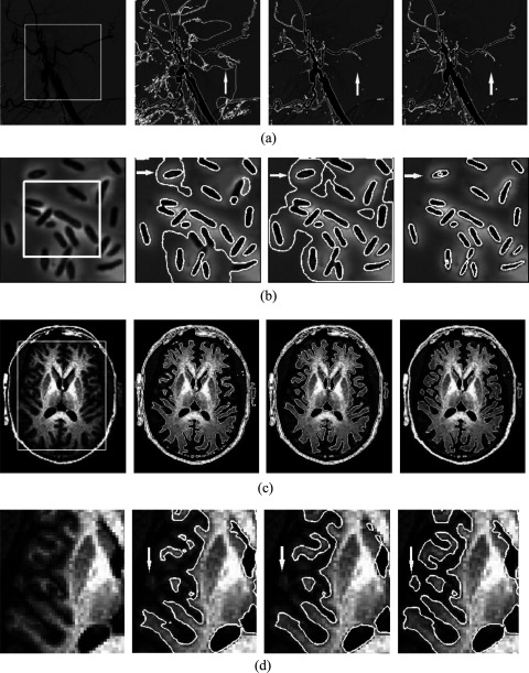
Figure 1 shows the segmentation results in a digital subtraction vessel image, electronic microscope chromosomal image, and brain MR image. The first column shows the original images with initial contours and the next three columns show the results of the RSF model, the GCS model, and our method. In this study, we used the scale parameter σ = 10 for the RSF model as it was recommended in the source code, and empirically used μ = 1000 and λ = 7000 for the GCS model.

FIG. 1.

Segmentation results on (a) digital subtraction vessel image using RSF model (second column), GCS model (third column), and our method (fourth column), (b) electronic microscope chromosomal image, and (c) brain MR image. (d) shows the enlarged view of the middle left portion of (c). The white curves indicate the outlines of the segmented regions, and the white arrows represent the locations where the three segmentation methods provided markedly different results.

Figure 1(a) shows segmentation results of the digital substation vessel image. It is apparent that the RSF model did not segment the vessel correctly because of the local minimum. In contrast, the GCS model and our method obtained good segmentation results with comparable accuracy.

Figure 1(b) shows segmentation results of the electron microscope chromosomal image with intensity inhomogeneity around the chromosomes. Although the RSF model has the ability to overcome intensity inhomogeneity, it could not segment chromosomes accurately, because it needs appropriate initial contours for a large number of objects in one image. We tested different initial contours for RSF. However, none of them could lead to acceptable results. Despite the fact that the GCS model is not dependent on the initial contours, it could not segment the chromosomes correctly, because of severe intensity inhomogeneity. On the other hand, our method correctly segmented the image with relatively high accuracy.

Figure 1(c) shows a comparison of the segmentation for a brain MR image. Both the RSF model and GCS model obtained acceptable segmentation results. The two methods, however, missed some gray matter regions near the skull, while our method segmented the gray matter accurately as shown in Fig. 1(d), which is the enlarged view of the middle left portion of (c).

III.B. Quantitative evaluation on synthetic image dataset

To quantitatively evaluate the proposed method, we applied the proposed method to a synthetic image dataset with different intensity inhomogeneity and noise levels. We also investigated the impact of the initial contour on the segmentation results on this dataset. Results from the RSF model and the GCS model were also provided for comparison.

We randomly generated 20 images with 7 circular objects for these experiments. The boundaries of these objects were known and used as the reference standards. These images were 8 bit grayscale images. The intensity contrast between the object and the background was 140. We added intensity inhomogeneity to the images by performing a linear intensity transformation along horizontal direction. The degree of the intensity inhomogeneity was defined as the intensity difference between the leftmost pixel and the rightmost pixel along horizontal direction in the image. Meanwhile, Gaussian noise with a mean of zero and different variances was added to the images. Please note that the pixel values of images were normalized to a range between 0 and 1 before adding the noise. We calculated the average overlap rates of the 20 simulated images.

We used the exhaustive searching method to determine the optimal parameter settings for the RSF and GCS models in all three experiments. For the RSF model, we searched the optimal value of σ in a relatively large range from 3 to 15 with an increment of 1. The range of values for λ₁ and λ₂ was 1, 1.2, 2, 3, and the range of values for υ was 0.001 × 255 × 255, 0.002 × 255 × 255, and 0.003 × 255 × 255. The optimal parameters searched from the above values for the RSF were: σ = 15, λ₁ = 1, λ₂ = 2, υ = 0.001 × 255 × 255. For the RSF model, μ and Δt were considered to be less important than the above four parameters and were assigned the RSF's default values of 1 and 0.1, respectively. Similarly, we determined the parameters μ and λ for the GCS model, which were 10 and 120, respectively.

III.B.1. Effect of initial contours

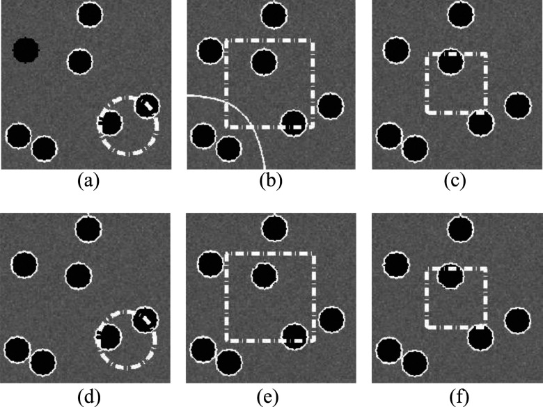
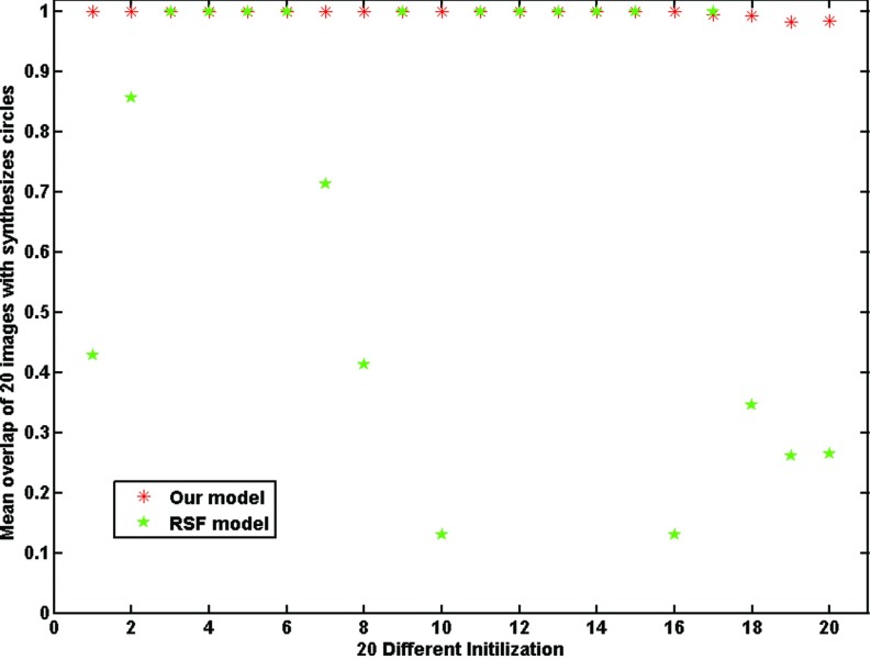
Because GCS model has the global convergence ability and is not dependent on initial contours, it was not included in this experiment. We applied our model and the RSF model to the testing images with 20 different initial contours. The testing images contained Gaussian noise with a variance of σ² = 0.005. Intensity inhomogeneity was not applied to these images. Figure 2 shows the segmentation results of an image with three different initial contours (green dashed contours) and their corresponding results (red solid contours) using RSF model and our model. It is apparent that the RSF model did not segment the objects accurately with the first two initial contours [Figs. 2(a) and 2(b)] due to the local minimum, while it successfully segmented the image with the third initial contour [Fig. 2(c)] Our model obtained good segmentation results with all the three different initial contours. The overlap rates of these two models with 20 different initial contours are shown in Fig. 3. The overlap rates of RSF model were distributed in a wide range between 10% and 100%. Thus, the RSF model is very sensitive to the initial contours. On the other hand, our model achieved consistently higher overlap rates (close to 99%) for all the initial contours. This result demonstrated that the proposed model is a reliable segmentation method with less dependence on the initial contours.

FIG. 2.

The segmentation results of RSF model [(a)–(c)] and our method [(d)–(f)] for a synthetic image with three different initial contours. The white dashed lines and solid lines represent the initial contours and the final contours, respectively.

FIG. 3.

Comparison of the RSF model and our model in terms of overlap rates for 20 different initializations.

III.B.2. Effect of intensity inhomogeneity

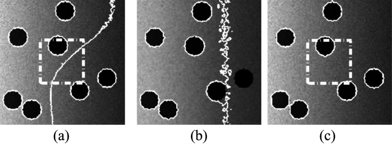
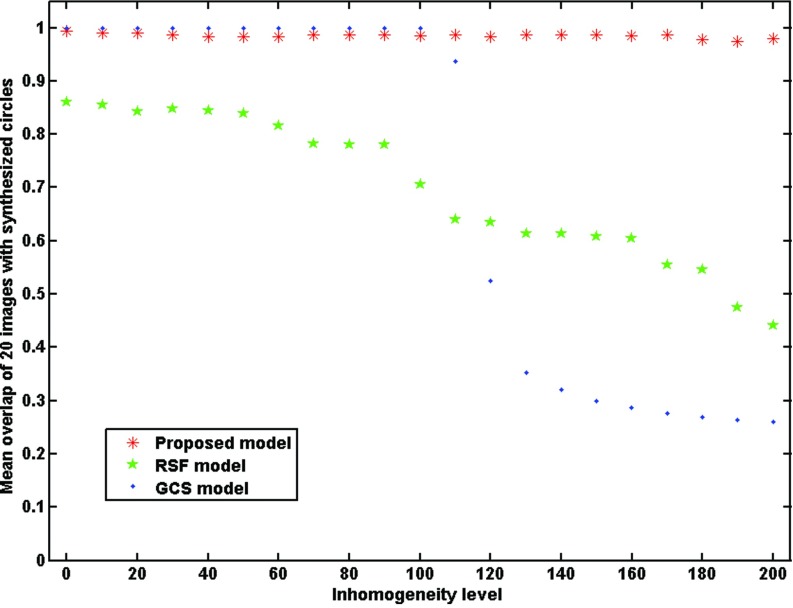
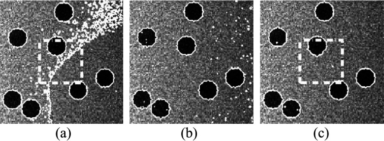
Twenty-one synthetic images with different intensity inhomogeneity degrees from 0 to 120 and the Gaussian noise variance of 0.005 were created for testing the effect of intensity inhomogeneity. The initial contour for RSF model and our model were shown in Figs. 2(c) and 2(f). Figure 4 shows the segmentation results from the RSF model [Fig. 4(a)], the GCS model [Fig. 4(b)], and our model [Fig. 4(c)] on a sample image with an intensity inhomogeneity degree of 120. It is apparent that neither the RSF model nor the GCS model segmented the image successfully, while our model achieved accurate segmentation result. Figure 5 shows the overlap rates of the three models for the 21 images. The GCS model obtained high overlap rate when the intensity inhomogeneity degree was lower than 110. As the intensity inhomogeneity degree increased, the overlap rate of both the RSF model and the GCS model decreased considerably, whereas our model consistently achieved very high overlap rate (>98%).

FIG. 4.

Segmentation results from (a) RSF model, (b) GCS model, and (c) our model on a synthetic image with an intensity inhomogeneity degree of 120.

FIG. 5.

Comparison of the RSF model, the GCS model, and our model in terms of overlap rates for images with different intensity inhomogeneity degrees.

III.B.3. Effect of noise

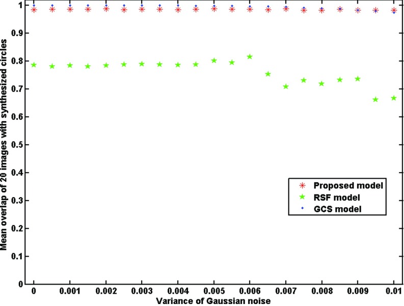
Twenty-one synthetic images with intensity inhomogeneity degree of 20 and different Gaussian noise variances between 0 and 0.01 were created for testing the effect of image noise. The initial contour for RSF model and our model were shown in Fig. 2. Figure 6 shows the segmentation results from the RSF model [Fig. 6(a)], the GCS model [Fig. 6(b)], and our model [Fig. 6(c)] on a sample image with an image noise variance of 0.01. As shown in Fig. 6(a), the RSF model did not obtain an acceptable segmentation result, while the GSC model and our model achieved good segmentation results with comparable accuracy. Figure 7 shows the overlap rates of three models for the 21 images with different Gaussian noise. As the Gaussian noise increased, the overlap rate of the RSF model decreased, and maintained between 65% and 85%. When the noise was low, the overlap rate of the GCS model was slightly higher than that of our model, whereas when the noise was high, the overlap rate of our model was slightly higher than that of the GCS model, nevertheless, both models achieved the overlap rate of greater than 97%.

FIG. 6.

Segmentation results from (a) RSF model, (b) GCS model, and (c) our model on a synthetic image with noise variance of 0.01.

FIG. 7.

Comparison of the RSF model, the GCS model and our model in terms of overlap rate for images with different image noise degrees.

III.C. Application to CT brain image segmentation

The main application of this study was the CSF segmentation in brain CT images, which is a critical step in the computer-aided detection of ischemic stroke in brain CT images.

The IRB of this study has been obtained at Duke University. We applied our model to the CT images and quantitatively evaluated the accuracy of segmentation results. The ranges for scale parameter σ, weighting factors λ₁, λ₂, and υ were the same as those in Sec. III B. We used the exhaustive searching method to obtain the optimal parameters for the RSF model: σ = 7, λ₁ = 1.2, λ₂ = 1, υ = 0.001 × 255 × 255. The μ and Δt were assigned the default value of 1 and 0.1, respectively. Similarly, we determined the optimal parameters μ and λ for the GCS model, which were 10 and 110, respectively.

Our dataset consists of 160 slices from 5 CT scans. The data used in this study were collected from the Duke University Medical Center. The CT slices of all subjects were acquired by use of 16-row (Light Speed 16, GE Medical System) CT scanners with an x-ray tube voltage of 120 KVp and a radiographic exposure of 120 mAs. The slice thickness is 5 mm. Each slice has a matrix size of 512 × 512 pixels and the pixel size is 0.4269 mm with a 16-bit gray level in Hounsfield unit (HU).

A reference standard of CSF was established to assess the accuracy of the segmentation result. A medical physicist (XQ, 4 years of experience) manually delineated the CSF boundaries for all the slices on a LCD screen. The delineated CSF was then confirmed or revised by an experienced medical physicist (QL, 15 years of experience).

Some preprocessing was carried out prior to this experiment. First, we manually extracted 67 slices from the 5 scans for this experiment. These selected slices contained the main part of the brain. We then automatically segmented the skull by use of a fixed CT value threshold of 56. The region inside the skull was defined as brain region and the region outside the skull was defined as background. Finally, the images were filtered by a median filter.

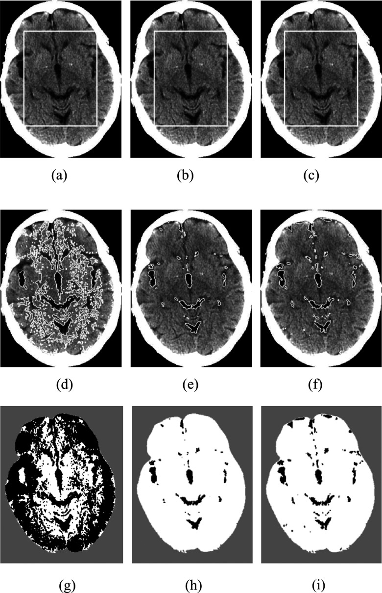
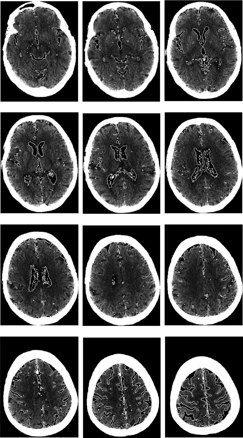
Figure 8 shows segmentation results obtained from the RSF model [Fig. 8(d)], the GCS model [Fig. 8(e)], and our model [Fig. 8(f)] on a sample CT slice. For the result of RSF model, many gray matter regions were incorrectly segmented as CSF. Although the segmentation result of the GCS model was comparable to that of our model, it missed some CSF regions close to the skull. Figure 9 shows the segmentation result of a CT scan obtained by our method. Our model segmented the CSF regions with high contrast and successfully excluded the calcification regions in the ventricle; it also correctly segmented low contrast CSF regions close to the skull by overcoming the intensity inhomogeneity caused by the cupping artifact.

FIG. 8.

Comparison of our model with the RSF model and the GCS model on a CT brain image. The three rows show the initial contours, the final contours, and the binary segment results. Column 1: RSF model, column 2: GCS model, column 3: our model. The results of the RSF model and the GCS model are their best results by use of many different combinations of parameters.

FIG. 9.

The results of our model for a CT scan. The final results were presented by the white solid curves.

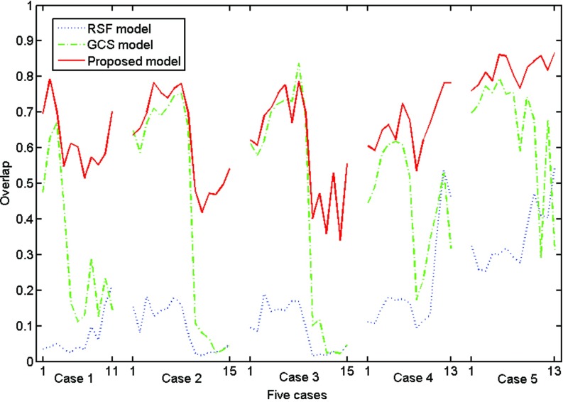
The overall overlap rates of the segmentation results obtained from the three models for all 67 slices were shown in Fig. 10. The overlap rates of our model were considerably higher than those of the RSF model for all slices and higher than GCS model in most of the slices, especially when the ventricle regions were absent in the slices. The red solid curve of case 4 in Fig. 10 presented the overlap rates of segmentation results shown in Fig. 9.

FIG. 10.

Comparison of overlap rates for the CSF segmentation in all slices in the five CT scans by the RSF model, the GCS model and our model.

Table I shows the mean, standard deviation, and the range of overlap rates for the RSF model, the GCS model, and our model. The mean overlap rates for the three models were 16.24%, 46.16%, and 66.47%. By use of two-tailed t-tests for the paired data, we found that our model achieved significantly better performance level than the RSF model (p < 0.001) and the GCS model (p < 0.001).

TABLE I.

The mean, standard deviation, and range of the overlap rate for CSF segmentation in brain CT images by the RSF model, the GCS model and our model.

	Mean	SD	Min	Max
RSF	0.1624a	0.0183	0.0157	0.5438
GCS	0.4616b	0.0721	0.0225	0.8379
Our model	0.6647a,b	0.0171	0.3409	0.8674

^ap < 0.001.

^bp < 0.001.

IV. DISCUSSION

Segmentation methods based on conventional active contour models are usually sensitive to the initial contour, intensity inhomogeneity, and image noise. In this study, we proposed a novel region-based active contour model that can overcome these challenges. The major advantage of our method is its insensitivity to the contour initialization as a result of magnification of the energy in the boundary regions of objects.

An additional strength of our method is that it is robust to image noise and intensity inhomogeneity and can obtain better results than the RSF model and GCS model. As the intensity inhomogeneity degree increased, the segmentation accuracy of RSF model declined gradually, while our method was able to successfully segment objects with high accuracy. The GCS model is evolved from the CV model and can obtain global optimal segmentation results. For images with noise or mild intensity inhomogeneity, both of the GCS model and our method achieved good segmentation results, whereas for the images with severe intensity inhomogeneity, our method achieved considerably better results than the GCS model.

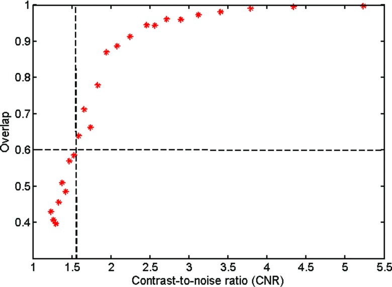
We further investigated the level of contrast-to-noise ratio at which the proposed method can achieve good segmentation performance. The contrast-to-noise ratio (CNR) is defined as the ratio of the intensity contrast between the foreground and the background and the standard deviation of the image noise. Figure 11 shows the segmentation accuracy, in terms of overlap rate, of the simulated images in Fig. 2 with different CNRs ranging from 1 to 6. As expected, the overlap rate of proposed method was improved as the CNR increased. When the CNR was greater than 1.6, the proposed method achieved acceptable segmentation results with overlap rates greater than 0.6; when the CNR further increased to 2.0 or above, the proposed method achieved good segmentation results with overlap rates greater than 0.8.

FIG. 11.

The segmentation accuracy of the proposed method for different contrast-to-noise ratios in terms of overlap rates.

As a limitation, our method could not well segment the small objects with low contrast. The reason of this issue is that the range domain function assigns very small weights to pixels near edges of low contrast. For instance, some tiny vessels with very low contrast in Fig. 1(a) were not correctly segmented by our method. However, as shown in Figs. 1(c) and 10 the overall segmentation obtained from our method is still much better than that from the conventional RSF and GCS models. Therefore, our method has great potential in the segmentation of complex medical images with acceptable accuracy. In the future, we may incorporate an additional region growing-based refinement step for picking up the weak edges that are missed by the proposed method.

For the segmentation of CSF, our method missed some CSF regions near the skull boundary because of strong image noise and relatively low contrast of CSF. In particular, some CSF regions may even have higher intensity (brighter) than that of the white matter due to the cupping artifact. However, because our method obtained an average overlap rate of 66% for the segmentation of the entire brain CT dataset and segmented the main parts of CSF very well, our method is a reliable segmentation tool for the brain CT images.

V. CONCLUSION

Accurate segmentation of CSF is not only clinically important, but also technically challenging. In this study, we developed a novel region-based active contour model. This method is robust to intensity inhomogeneity and image noise, as well as insensitive to the initial contours. The experimental results have demonstrated that the proposed method could obtain segmentation results with high accuracy compared to the conventional RSF and GCS models. Overall, this method provided an automated CSF segmentation tool for the brain CT studies of acute ischemic stroke and would be useful for the development of CAD schemes for acute ischemic stroke.

REFERENCES

- 1.Takahasi N., Tsai D. Y., Lee Y., Kinoshita T., and Ishii K., “Z-score mapping method for extracting hypoattenuation areas of hyperacute stroke in unenhanced CT,” Acad. Radiol. 17, 84–92 (2010). 10.1016/j.acra.2009.07.011 [DOI] [PubMed] [Google Scholar]
- 2.Takahashi N., Lee Y., Tsai D. Y., Ishii K., Kinoshita T., Tamura H., and Kimura M., “Improvement of detection of hypoattenuation in acute ischemic stroke in unenhanced computed tomography using an adaptive smoothing filter,” Acta Radiol. 49, 816–826 (2008). 10.1080/02841850802126570 [DOI] [PubMed] [Google Scholar]
- 3.Przelaskowski A., Sklinda K., Bargieł P., Walecki J., Biesiadko-Matuszewska M., and Kazubek M., “Improved early stroke detection: Wavelet-based perception enhancement of computerized tomography exams,” Comput. Biol. Med. 37, 524–533 (2007). 10.1016/j.compbiomed.2006.08.004 [DOI] [PubMed] [Google Scholar]
- 4.Balafar M. A., Ramli A. R., Saripan M. L., and Mashohor S., “Review of brain MRI image segmentation methods,” Artif. Intell. Rev. 33, 261–274 (2010). 10.1007/s10462-010-9155-0 [DOI] [Google Scholar]
- 5.Li C., Huang R., Ding Z., Gatenby J. C., and Metaxas D. N., “A level set method for image segmentation in the presence of intensity inhomogeneities with application to MRI,” IEEE Trans. Image Process. 20, 2007–2016 (2011). 10.1109/TIP.2011.2146190 [DOI] [PMC free article] [PubMed] [Google Scholar]
- 6.Wang L., Li C., Sun Q., Xia D., and Kao C., “Active contours driven by local and global intensity fitting energy with application to brain MR images segmentation,” Comput. Med. Imaging Graph. 33, 520–531 (2009). 10.1016/j.compmedimag.2009.04.010 [DOI] [PubMed] [Google Scholar]
- 7.Wang L., Shi F., Lin W., Gilmore J. H., and Shen D., “Automatic segmentation of neonatal images using convex optimization and coupled level sets,” NeuroImage 58, 805–817 (2011). 10.1016/j.neuroimage.2011.06.064 [DOI] [PMC free article] [PubMed] [Google Scholar]
- 8.Yang X. and Fei B., “A multiscale and multiblock fuzzy c-means classification method for brain MR images,” Med. Phys. 38, 2879–2891 (2011). 10.1118/1.3584199 [DOI] [PMC free article] [PubMed] [Google Scholar]
- 9.Wang H. and Fei B., “A modified fuzzy c-means classification method using a multiscale diffusion filtering scheme,” Med. Image Anal. 13, 193–202 (2009). 10.1016/j.media.2008.06.014 [DOI] [PMC free article] [PubMed] [Google Scholar]
- 10.Kumazawa S., Yosiura T., Honda H., Toyofuku F., and Higasida Y., “Partial volume estimation and segmentation of brain tissue based on diffusion tensor MRI,” Med. Phys. 37, 1482–1490 (2010). 10.1118/1.3355886 [DOI] [PubMed] [Google Scholar]
- 11.Li X., Li L., Lu H., and Liang Z., “Partial volume segmentation of brain magnetic resonance images based on maximum a posterior probability,” Med. Phys. 32, 2337–2345 (2005). 10.1118/1.1944912 [DOI] [PubMed] [Google Scholar]
- 12.Wei K., He B., Zhao T., and Shen X., “A novel method for segmentation of CT head images,” in Proceedings of the IEEE Computer Society Conference on Bioinformatics and Biomedical Engineering (ICBBE), Wuhan, China (IEEE, Piscataway, NJ, 2007), pp. 717–720 [Google Scholar]
- 13.Lee T. H., Fauzi M. F. A., and Komiya R., “Segmentation of CT brain images using K-means and EM Clustering,” in Proceedings of the IEEE Fifth International Conference on Computer Graphics, Imaging and Visualization, Penang, Malaysia (IEEE CS, Washington, DC, 2008), pp. 339–344 [Google Scholar]
- 14.Chen W. and Najarian K., “Segmentation of ventricles in brain CT images using Gaussian mixture model method,” in Proceedings of the IEEE International Conference on Complex Medical Engineering, Tempe, AZ (IEEE, Piscataway, NJ, 2009), pp. 15–20 [Google Scholar]
- 15.Gupta V., Ambrosius W., Qian G., Blazejewska A., Kazmierski R., Urbanik A., and Nowinski W. L., “Automatic segmentation of cerebrospinal fluid, white and gray matter in unenhanced computed tomography images,” Acad. Radiol. 17, 1350–1358 (2010). 10.1016/j.acra.2010.06.005 [DOI] [PubMed] [Google Scholar]
- 16.Chen W., Smith R., Ji S., Ward K. R., and Najrian K., “Automated ventricular systems segmentation in brain CT images by combining low-level segmentation and high-level template matching,” BMC Med. Inf. Decis. Making 9, 1–14 (2009). 10.1186/1472-6947-9-S1-S4 [DOI] [PMC free article] [PubMed] [Google Scholar]
- 17.Liu J., Huang S., Ihar V., Ambrosius W., Lee L. C., and Nowinski W. L., “Automatic model-guided segmentation of the human brain ventricular system form CT images,” Acad. Radiol. 17, 718–726 (2010). 10.1016/j.acra.2010.02.013 [DOI] [PubMed] [Google Scholar]
- 18.Suzuki K., Kohlbrenner R., Epstein M. L., Obajuluwa A. M., Xu J., and Hori M., “Computer-aided measurement of liver volumes in CT by means of geodesic active contour segmentation coupled with level-set algorithms,” Med. Phys. 37, 2159–2166 (2010). 10.1118/1.3395579 [DOI] [PMC free article] [PubMed] [Google Scholar]
- 19.Vandemeulebroucke J., Bernard O., Clarysse P., Rit S., Sarrut D., and Kybic J., “Automated segmentation of a motion mask to preserve sliding motion in deformable registration of thoracic CT,” Med. Phys. 39, 1006–1015 (2012). 10.1118/1.3679009 [DOI] [PubMed] [Google Scholar]
- 20.Tao Y., Lo S. B., Freedman M. T., Makariou E., and Xuan J., “Multilevel learning-based segmentation of ill-defined and speculated masses in mammograms,” Med. Phys. 37, 5593–6002 (2010). 10.1118/1.3490083 [DOI] [PMC free article] [PubMed] [Google Scholar]
- 21.Caselles V., Kimmel R., and Sapiro G., “Geodesic active contours,” Int. J. Comput. Vis. 22, 61–79 (1997). 10.1023/A:1007979827043 [DOI] [Google Scholar]
- 22.Dindoyal I., Lambrou T., Deng J., and Pokropek A. T., “2D/3D fetal cardiac dataset segmentation using a deformable model,” Med. Phys. 38, 4338–4349 (2011). 10.1118/1.3592638 [DOI] [PubMed] [Google Scholar]
- 23.Duan C., Liang Z., Bao S., Zhu H., Wang S., Zhang G., Chen J. J., and Liu H., “A coupled level set framework for bladder wall segmentation with application to MR cystography,” IEEE Trans. Med. Imaging 29, 903–915 (2010). 10.1109/TMI.2009.2039756 [DOI] [PMC free article] [PubMed] [Google Scholar]
- 24.Yazdanpanah A., Hamarneh G., Smith B. R., and Sarunic M. V., “Segmentation of intra-retinal layers from optical coherence tomography images using an active contour approach,” IEEE Trans. Med. Imaging. 30, 484–496 (2011). 10.1109/TMI.2010.2087390 [DOI] [PubMed] [Google Scholar]
- 25.Chan T. and Vese L., “Active contours without edges,” IEEE Trans. Image Process. 10, 266–277 (2001). 10.1109/83.902291 [DOI] [PubMed] [Google Scholar]
- 26.Goldstein T., Bresson X., and Osher S., “Geometric applications of the split Bregman method: Segmentation and surface reconstruction,” J. Sci. Comput. 45, 272–293 (2010). 10.1007/s10915-009-9331-z [DOI] [Google Scholar]
- 27.Li C., Kao C., Gore J. C., and Ding Z., “Minimization of region-scalable fitting energy for image segmentation,” IEEE Trans. Image Process. 17, 1940–1949 (2008). 10.1109/TIP.2008.2002304 [DOI] [PMC free article] [PubMed] [Google Scholar]
- 28.Lankton S. and Tannenbaum A., “Localizing region-based active contours,” IEEE Trans. Image Process. 17, 2029–2039 (2008). 10.1109/TIP.2008.2004611 [DOI] [PMC free article] [PubMed] [Google Scholar]
- 29.Tomasi C. and Manduchi R., “Bilateral filtering for gray and color images,” in Proceedings of the IEEE International Conference on Computer Vision, Bombay, India (IEEE, Piscataway, NJ, 1998), pp. 839–846 [Google Scholar]
- 30.Osher S. and Shah J., “Fronts propagating with curvature-dependent speed: algorithms based on Hamilton-Jacobi formulations,” J. Comput. Phys. 79, 12–49 (1988). 10.1016/0021-9991(88)90002-2 [DOI] [Google Scholar]
- 31.Li C., Xu C., Gui C., and Fox M. D., “Distance regularized level set evolution and its application to image segmentation,” IEEE Trans. Image Process. 19, 3243–3254 (2010). 10.1109/TIP.2010.2069690 [DOI] [PubMed] [Google Scholar]