Efficient Spatiotemporal Analysis of the Flagellar Waveform of Chlamydomonas reinhardtii

Abstract

The 9 + 2 axoneme is a microtubule-based machine that powers the oscillatory beating of cilia and flagella. Its highly regulated movement is essential for the normal function of many organs; ciliopathies cause congenital defects, chronic respiratory tract infections and infertility. We present an efficient method to obtain a quantitative description of flagellar motion, with high spatial and temporal resolution, from high speed video recording of bright field images. This highly automated technique provides the shape, shear angle, curvature, and bend propagation speeds along the length of the flagellum, with ∼200 temporal samples per beat. We compared the waveforms of uniflagellated wild-type and ida3 mutant cells, which lack the I1 inner dynein complex. Video images were captured at 350 fps. Rigid-body motion was eliminated by fast Fourier transform (FFT)-based registration, and the Cartesian (x–y) coordinates of points on the flagellum were identified. These x–y “point clouds” were embedded in two data dimensions using Isomap, a nonlinear dimension reduction method, and sorted by phase in the flagellar cycle. A smooth surface was fitted to the sorted point clouds, which provides high-resolution estimates of shear angle and curvature. Wild-type and ida3 cells exhibit large differences in shear amplitude, but similar maximum and minimum curvature values. In ida3 cells, the reverse bend begins earlier and travels more slowly relative to the principal bend, than in wild-type cells. The regulation of flagellar movement must involve I1 dynein in a manner consistent with these results.

Introduction

Dyneins are minus-end directed microtubule motors that provide force for a variety of cellular processes. Dynein arms generate flagellar and ciliary motion by conversion of ATP hydrolysis into microtubule sliding. The flagellar axoneme consists of a central pair apparatus of two singlet micro-tubules and projections, surrounded by nine doublet microtubules that anchor outer dynein arms (ODA), inner dynein arms (IDA) and radial spokes (RS). These structures act together to generate a coordinated, repeating waveform [Wirschell and Sales, 2007]. The unicellular alga, Chlamydomonas reinhardtii, provides an excellent experimental system to understand how ciliary/flagellar waveforms are generated. Most of the early analysis of the waveform of Chlamydomonas flagella was aided by the uni1 mutant strain [Huang et al., 1982]. The uni1 mutant strain assembles only one flagellum, and uni1 cells that use the “breast-stroke” or forward movement mode rotate in place in a plane perpendicular to the axis of rotation [Brokaw et al., 1982]. Beginning with Brokaw and Luck [1983], flagella were photographed using dark field optics with flash illumination at 300 Hz, and four to eight images covering a single beat were analyzed.

Dynein motors promote sliding of adjacent outer doublet microtubules that is converted into bending and oscillatory beating [Summers and Gibbons, 1971]. Mutations in at least 10 genes in Chlamydomonas result in the loss of the outer dynein arms, which are located on the outer circumference of the doublet microtubules. Loss of the outer dynein arms affects the frequency of the beat [Brokaw and Kamiya, 1987; King and Kamiya, 2008]. The inner dynein arms, which are located on the inner circumference, are heterogeneous [Wirschell and Sales, 2007]. There are at least seven dynein isoforms that bind to the microtubule B-tubule in a 96 nm pattern that essentially repeats, with some differences, along the length of the flagellar axoneme [Piperno et al., 1990; Nicastro et al., 2006; King and Kamiya, 2008]. The loss of the best-studied inner dynein arm, called I1 or ƒ dynein, is known to affect the waveform [Brokaw and Kamiya, 1987]. The I1 inner dynein is a two-headed dynein that is found along the length of the axoneme and appears as a tri-lobed structure by electron microscopy [Nicastro et al., 2006].

The I1-dynein complex is likely to be a target of regulatory signals that control the flagellar waveform [Porter et al., 1992; Porter and Sale, 2000; Smith and Yang, 2004; Wirschell and Sales, 2007]. Flagella that are lacking I1 dynein exhibit defective flagellar waveform and phototaxis, which indicates that I1 dynein plays a role in these processes [Brokaw and Kamiya, 1987; Brokaw, 1994; King and Dutcher, 1997; Okita et al., 2005]. At least some of this regulation is conferred by changes in the phosphorylation state of IC138, which is a phosphoprotein and is a key substrate for the regulatory mechanisms that control flagellar motility [reviewed in Porter and Sale, 2000; Wirschell and Sales, 2007].

The ability to isolate mutants in Chlamydomonas has outpaced the ability to efficiently and precisely describe the flagellar waveform. Qualitative differences in waveform among different mutants are frequently noted [Dutcher et al., 1988; King et al., 1994; Bower et al., 2009], but since the seminal work of Brokaw, Kamiya and collaborators [Brokaw et al., 1982; Huang et al., 1982; Brokaw and Luck, 1983; Brokaw, 1984; Brokaw and Kamiya, 1987] few authors have provided quantitative measurements. This lack may occur because analysis of Chlamydomonas waveform has generally been labor-intensive and difficult to perform. Notably, Rüffer and Nultsch performed a series of studies [e.g., Rüffer and Nultsch, 1985, 1987, 1990, 1991] in which Chlamydomonas flagella were filmed at 500 frames per second (fps), but flagella were traced by hand. Brokaw [1990] developed an automated method to characterize the waveform of sperm flagella; the different features of the Chlamydomonas body and flagellar waveform prevent the direct application of this method. In addition, the flash illumination technology and dark field optics used in Brokaw's work is challenging to deploy, compared to simple bright field imaging.

We report a new method for acquiring and analyzing flagellar waveforms. This technique is motivated by the desire to efficiently, precisely, and objectively describe the active bending process. The ability to make these observations with high spatial and temporal resolution will help illuminate the coordination of dynein activity that produces the normal and abnormal flagellar waveform. It is now possible to acquire extensive high-speed video of flagellar motion with inexpensive digital camera systems and bright field optics. Here we focus on the extraction of a physically meaningful description of the flagellar waveform from high-speed video image data. We demonstrate the utility of this approach by comparison of the flagellar waveform in wild-type Chlamydomonas and in a mutant (ida3) lacking the I1-dynein complex.

Materials and Methods

Cell Cultures and Genetics

Chlamydomonas reinhardtii cells were grown as previously described [Holmes and Dutcher, 1989]. The uniflagellate mutant strains, uni1-2 and uni1-2; ida3, were generated from meiotic crosses, as described by Dutcher [1995]. The uni1-2 strain was utilized for its ability to rotate in place, which allows for easier filming and data collection [Brokaw et al., 1982]. Mutants displaying the ida3 phenotype were selected from meiotic progeny of a uni1-2 by ida3 cross by screening for cells that rotated more slowly than the uni1-2 cells. Selected double mutant strains were confirmed by backcrossing with wild-type cells and analyzing the meiotic progeny. The uni1-2 and uni1-2; ida3 cells were allowed to grow for 48 h in Sager and Granick rich liquid medium [Lux and Dutcher, 1991] at 25°C in constant light before filming.

Video Microscopy

All bright field microscopy was carried out in a climate-controlled room maintained at 21°C. For each video, 20 μL from a liquid culture were pipetted onto an acid washed slide and a coverslip was placed for viewing under a Zeiss Universal Microscope (Carl Zeiss, Oberkochen, Germany) with either 63× Planapo or 100× Neofluar oil-immersion objective lenses. As soon as a single, rotating cell was brought into focus, microscope settings were adjusted to provide the greatest contrast between the flagellum and background. Videos were made using the Dragonfly Express IEEE-1394b Digital Camera System and FlyCapture software (Point Grey Research, Scottsdale, AZ). Videos were captured at ∼350 frames per second with 320 × 240 resolution. The shutter speed was 2.88 ms. Each video was 600 frames in length, or roughly 1.7 s long and was recorded in AVI format.

Analysis Protocol

Videos were analyzed with custom programs written in Matlab™ (The Mathworks, Natick, MA). From each video, a sequence of M (typically 200) consecutive frames was stored as a “stack” of images, which is a three-dimensional array (320 × 240 × M) of intensity values. The resolution of this array was 0.12 μm in the two spatial dimensions and 2.9 ms in the temporal dimension. (The Matlab programs are available by email upon request).

The analysis consists of four major steps. First, we characterize, and subtract the gross (“rigid-body”) motion of the cell body (Fig. 1) so that the flagellar motion can be described with respect to a fixed reference frame with its origin at the proximal end of the flagellum (Figs. 2a and 2b). Second, we identify the Cartesian (x,y) coordinates, with respect to this fixed frame, of a specified number of pixels on the flagellum, which generates a 2D, flagellum-shaped, “cloud” of points, from each video image (Fig. 2c). Third, we sort the flagellar point clouds in order of their presumed phase in the beat cycle (Fig. 3). Finally, the sorted clouds of points are fit to a smooth, time-periodic surface of shear angle as a function of time and space (Figs. 4 and 5). Parameters of motion, such as curvatures, sliding velocities, and delay times, can be extracted from these surfaces. These are directly comparable to the analogous parameters estimated by Brokaw, Kamiya and their collaborators [Brokaw et al., 1982; Huang et al., 1982; Brokaw and Luck, 1983; Brokaw, 1984; Brokaw and Kamiya, 1987].

Fig. 1.

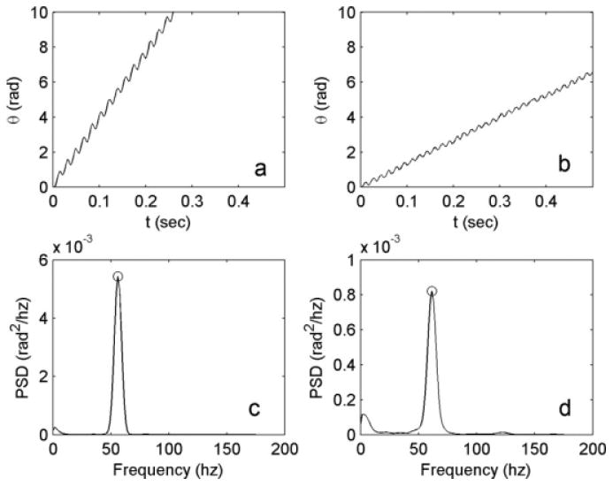
(a) Angle of rigid body rotation observed in a video of wild-type uni1-2 Chlamydomonas. Mean rotation rate is 6.13 revolutions per second. (b) Angle of rigid body rotation observed in a video of an ida3 mutant cell. Mean rotation rate is 2.08 revolutions per second. (c) Power spectral density function (PSD) of the oscillations in (a); the peak at 56.6 Hz represents the beat frequency of this wild-type cell. (d) Power spectral density function (PSD) of the oscillations in Fig. 2b, showing a beat frequency of 61.5 Hz for this ida3 cell.

Fig. 2. Overview of video analysis.

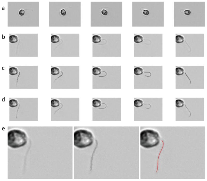
(a) Video frames after the image background has been subtracted. (b) Video images after rigid-body motion has been removed. (c) “Point clouds” of pixels identified as belonging to the flagellum, superimposed on the video frames. (d) Curves obtained from fitting of a polynomial function (Eq. 1) to the point clouds shown above. Curve fitting was done after the sorting procedure described in the text and illustrated in Fig. 3. (e) Enlarged views of the first images in rows (b–d).

Fig. 3. Sorting of flagellar point clouds.

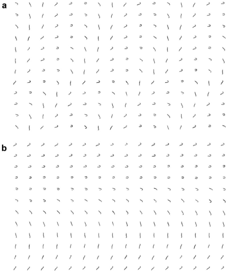
(a) Unsorted point clouds. (b) Point clouds after sorting by order of phase in flagellar cycle, as identified by isometric feature mapping (Isomap). The first six rows of the sorted beat correspond to “recovery” as the primary bend propagates from base to tip; the last six rows roughly correspond to the “power stroke” driven by propagation of the reverse bend.

Fig. 4.

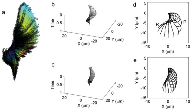
(a) Point clouds sorted and plotted on x–y-time coordinate axes, along with the smoothed surface of Cartesian coordinates obtained by the fitting procedure. (b,c) Line plots showing the waveforms for wild-type and ida3 respectively in 3D (x–y-time coordinates). (d,e) Successive “snapshots” of the flagellar waveforms in 2D (x–y coordinates) of wild-type and ida3 respectively. In (d,e), for clarity waveforms are shown only at intervals of 1/12 cycle. P indicates the “primary” bend as it approaches the end of the flagellum; R indicates the “reverse” bend.

Fig. 5. (a–c) Surfaces of shear angle θ(s,t) as a function of distance along the flagellum, s, and time throughout the cycle.

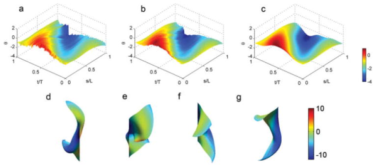
Distances are normalized by flagellar length, L, and time is normalized by the beat period, T. (a) An example surface constructed from unfiltered polynomial curves fitted to 200 point clouds. (b) The same surface after median filtering in time. (c) The same surface after median filtering and smoothing with gridfit; color represents shear angle. (d–g) Four different views of the Cartesian (x–y-time) surface corresponding to the smoothed θ(s,t) surface; color represents surface curvature.

These four steps are described in more detail in the following sections.

Correction of Rigid-Body Motion

In the first image, a rectangular region closely fitting the cell body is manually selected as the region of interest (ROI). This ROI is rotated by 0.5° increments to provide a set of 720 rotated template images. Each frame of the video is compared to each rotated template, using a fast Fourier transform (FFT)-based convolution procedure [Rosenfeld and Avinash, 1976]. This procedure finds the correlation between ROIs for a given rotation angle and relative displacement. The highest correlation across all rotated templates identifies the angle of rotation, and the displacement vector that produces the highest correlation between the template ROI and the corresponding ROI in the video frame. These angles and displacements are stored for subsequent steps. The rotation frequency and beat frequency are obtained from the time series of angular corrections (Fig. 1).

Identification of Cartesian Point Clouds from Images

The flagellum is visually identifiable because it is darker than the background (Fig. 2a); this property is used to identify flagellar pixels automatically. The static background of the video is subtracted to eliminate defects in the field of view. The rotation angles and displacement vectors identified above are applied to generate transformed (rotated and translated) images, using standard image processing software (imtransform, Matlab, The Mathworks, Natick, MA). Examples of images at this stage are shown in Fig. 2b. The rectangular region containing the dark flagellum is then selected from the entire image stack by manually outlining the region in one image.

The flagellum is the main source of contrast in the resulting images. A point cloud is generated by selecting the darkest N points (typically N = 100). In ∼90% of all images, the point cloud consists of N points that all lie on the flagellum in a fairly uniform proximal-distal distribution (Fig. 2c). In the remaining cases, a number of “false positive” points lie somewhere else on the image, away from the flagellum. The user has the option to selectively eliminate these points, and replace them manually with a point on the flagellum, using the Matlab graphical user interface (ginput). It should be noted that in all the images we obtain it is very difficult to reliably resolve the flagellum automatically in the most proximal segment (∼1 μm), because a bright “halo” typically surrounds the cell body. Analogous difficulties characterizing flagellar motion near the base were noted in the analysis of dark-field images described by Brokaw and Luck [1985]. Accordingly the analysis here begins at a point ∼ 1 μm from the cell body.

Sorting of Point Clouds using Isometric Feature Mapping

The point clouds represent snapshots of the flagellum at a large number of times, but the basic time resolution is coarse relative to the period of motion. However, the mismatch between beat frequency and sampling frequency, augmented by random small variations in beat frequency, causes the snapshots to be distributed fairly evenly over the beat cycle. In other words, a high-resolution representation of the beat can be obtained by sorting the coarse time samples in order of their phase in the cycle.

Points on the flagellum during a sequence of beats are not random, but lie on a surface, or “manifold” in space-time. The isometric feature mapping algorithm “Isomap,” developed by Tenenbaum et al. [2000] is designed to take unordered samples from an arbitrary, unknown, low-dimensional manifold and to return parameters that correspond to the location of the sample on that structure. Thus, Isomap is ideally suited for sorting point clouds from cyclical motion [Pless and Simon, 2002]. We define a difference measure between two point clouds as sum of the squared Euclidean distances between pairs of points (two point clouds are identical if this measure is zero). Isomap then determines which point clouds are neighbors, by checking if the difference measure between them is less than a specified value, ε. Isomap then connects the neighbors, forming a network, or “graph” [Tenenbaum et al., 2000]. Geodesic distances on the data manifold are estimated by computing the shortest paths between point clouds, traveling from neighbor to neighbor in this network. If the data truly originate from cyclical behavior, then the manifold is a closed curve and the geodesic paths between point clouds lie on the curve. Most importantly for the current study, the position along this curve represents the phase of the cycle [Pless, 2003]. The sorting of point clouds by this approach is demonstrated in Fig. 3.

Fitting of Curves and Surfaces

Since the Chlamydomonas flagellar waveform varies smoothly in both space and time, it may be described by a smooth surface in these dimensions. First, a simple polynomial function θ_m(s) (Eq. 1) is fitted to each of the M point clouds. Note that θ_m(s) = θ_m(s,t) at time t = t_m. The fit is performed by choosing the five coefficients (a_i) in Eq. 1 that minimize an “objective function,” J. The fourth-order polynomial form of Eq. 1 was chosen empirically as the simplest function that appears to capture the shape of the flagellum. Increasing to fifth-order did not noticeably improve the fit (data not shown).

$${\mathrm{\theta }}_m(s)=a_0+a_{1}s+a_2{s}^2+a_3{s}^3+a_4{s}^4,m=1,2,\dots ,M.$$ (1)

The first term in the objective function is the sum of the squared distances, d_n, from the each point in the point cloud to the closest point on the fitted curve. Equations 2 and 3 are used to compute the Cartesian coordinates of points on the fitted curve:

$$x(s,t)={\int }_0^{s}cos\mathrm{\theta }(s^{\prime },t){\mathit{\text{ds}}}^{\prime }$$ (2)

$$y(s,t)={\int }_0^{s}sin\mathrm{\theta }(s^{\prime },t){\mathit{\text{ds}}}^{\prime }.$$ (3)

To find each distance, the equations defining the curve (Eqs. 1–3) are evaluated at 100 values of axial position, s, to provide 100 Cartesian pairs (x_ci, y_ci) on the curve. For a given data point, (x_n, y_n) the Euclidean distance $\sqrt{{(x_n-x_{\mathit{\text{ci}}})}^2+{(y_n-y_i)}^2}$ from the selected data point to each of the points on the curve is calculated; the minimum of those distances is d_n, the distance from the data point to the curve. Penalty terms reflecting magnitude of curvature, $\mathrm{\kappa }=\frac{d\mathrm{\theta }}{\mathit{\text{ds}}}$, and deviation from an estimated proximal emergence angle, θ₀, are included in the objective function to provide physically-reasonable shapes. The curvature penalty captures the physical property of elasticity (flexural rigidity). It is quite possible to bend a beam into a very highly curved shape, but if the beam is stiff (resists curvature), it would take large physical forces to do so. The objective function is thus written, in general as,

$$J=w_1\sum _{n=1}^N{d}_n^2+w_2{\int }_0^L{\mathrm{\kappa }}^2\mathit{\text{ds}}+w_3{(a_0-{\mathrm{\theta }}_0)}^2$$ (4)

where w_i are weighting coefficients. In this study the first two terms in Eq. 4 are emphasized, since the primary goal is to accurately characterize the waveform in the main body of the flagellum. This combination of polynomial fit and objective function is simple and robust, and requires minimal time and user intervention. Minimization of the objective function was accomplished by the Nelder-Mead algorithm implemented in Matlab by the fminsearch routine. Fitting curves to 200 point clouds of 100 points each requires 10–15 min on a PC with 2.4 GHz CPU and 2.0 Gb RAM.

By assembling the curves θ_m(s) for all times t = t_m, we construct the surface θ(s, t) which represents the angle of the tangent to the curve as a function of distance along the flagellum (s) and time (t) (Fig. 4). After curves were fitted to all M point clouds, the functions were evaluated at N = 100 spatial points along the flagellum. The set of curves thus provides a dense distribution (N × M array) of points θ_nm = θ(s_n, t_m) on the hypothetical surface, θ(s, t) (Figs. 4 and 5). A median filter with a width of five points is applied in the time direction to remove outlying values of θ (outliers can be caused by outlying data, such as an aberrant image, or by a failed curve fit). The array is smoothed in both space and time dimensions using the function gridfit in Matlab, which maximizes the smoothness of the surface gradient (http://www.mathworks.com/matlabcentral/fileexchange/8998; J. D'Errico). Finally, a FFT-based filter is used to remove higher temporal harmonics (components at all frequencies greater than three times the fundamental beat frequency). Figure 5 illustrates the sequential smoothing of the shear angle surface by the median filter and gridfit function.

Characterization of Waveforms and Statistical Analysis

The steps described above reduce a large set of video image data (320 × 240 × M) to a much smaller array of points (N × M) that describe the surface θ(s, t) of flagellar angle versus space and time. We use the key features of this surface to try to illuminate the biophysics of flagellar motion. Following Brokaw and collaborators [Brokaw et al., 1982; Huang et al., 1982; Brokaw and Luck, 1983; Brokaw, 1984; Brokaw and Kamiya, 1987] we extract curvature $\mathrm{\kappa }=\frac{d\mathrm{\theta }}{\mathit{\text{ds}}}$, rate of change of angle, $V=\frac{d\mathrm{\theta }}{\mathit{\text{dt}}}$, and time delay between primary and reverse bend initiation, as well as the average amplitude of angular oscillation at each point. Average principal and reverse curvature values are calculated by scanning the curvature field to find the minimum (principal) and maximum (reverse) curvatures exhibited at each flagellar location (Fig. 8k illustrates the occurrence of these critical curvatures at the midpoint of the flagellum). These values are then averaged over the middle 80% of the flagellum (i.e., avoiding the proximal and distal extremes). The average sliding velocity in the principal or reverse bend is obtained similarly. The maximum and minimum rates of change of angle are found at each location, and the values are averaged over the middle 80% of the flagellum. Also, although straight and curved regions of the flagellum are not explicitly identified, we obtain the propagation velocity of curves by estimating the rate of change in the spatial positions of maxima and minima of curvature. Averages (mean) ± standard deviations of these parameters are reported in our Results section; statistical significance was evaluated using Student's t-test.

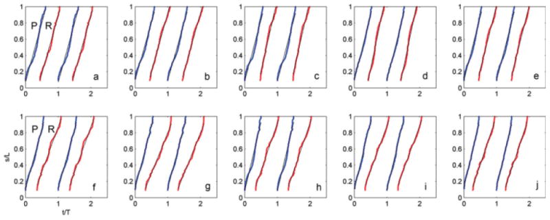
Fig. 8. Curvature $\mathrm{\kappa }=\frac{d\mathrm{\theta }}{\mathit{\text{ds}}}$ (normalized by flagellar length) plotted versus normalized time (t/T, horizontal axis) during the cycle and normalized distance along the flagellum (s/L, vertical axis), for five representative videos of wild-type (a–e) and ida3 cells (f–j).

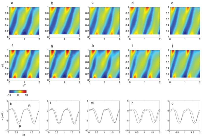
(k–o) Plots of curvature versus time at the midpoint of the flagellum, showing that the duration of high negative curvature is shorter in ida3 flagella (dashed) than in wild-type flagella (solid), although minimum curvature values are similar. Each pair of curves corresponds to the two maps above them. These maps and plots correspond to the waveforms of Fig. 6; note that two beat cycles are shown.

Results

Our objective is a parsimonious, quantitative, and objective description of flagellar motion from video images acquired with bright field optics. The methods developed by Brokaw and colleagues [1982, 1983, 1984, 1987] serve as a starting point for the present approach. A key feature of the new approach is that it provides significant improvement in the effective temporal resolution, which is achieved by acquisition of a large number of images from multiple beats, adjusting for the motion of the body, and by automatically sorting the data by its phase in the flagellar cycle.

Data Overview

All cells used in this analysis carry the uni1-2 mutation; therefore about 90% of the cells are uniflagellated and in rotate in place [Huang et al., 1982]. The flagellar waveforms from 12 uniflagellate (uni1-2) wild-type and 12 ida3; uni1-2 mutant cells were collected and analyzed. Five representative wild-type flagellar waveforms are shown in the top row of Fig. 6; these curves represent snapshots of the interpolated waveform at regular intervals of 1/12 of a cycle. The waveforms show common characteristics, as well as individual variations. All beats exhibit a recovery stroke in which the highly curved flagellum retracts while shear angles increase (counterclockwise rotation), and a propulsive power stroke in which the flagellum straightens and rotates clockwise. The recovery stroke is described by the propagation of a negative curvature band (the “principal bend,” P) from the proximal to distal end of the flagellum, and the power stroke by the subsequent propagation of a positive curvature band (“reverse bend,” R). The bottom row of Fig. 6 shows waveforms from the ida3 mutant. Both the recovery stroke and the power stroke appear abbreviated. These clear differences in global flagellar behavior motivated us to examine local measurements of flagellar shape and behavior, which might illuminate the causal biophysical mechanisms.

Fig. 6. Waveforms from five representative videos of wild-type (a–e) and ida3 mutant cells (f–j).

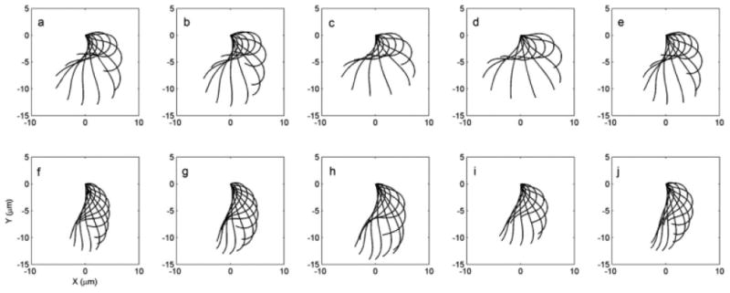
For clarity, waveforms are shown only every 1/12 of a cycle.

The comparison of wild-type and ida3 cells illustrate several similarities; these include the beat frequency (average 69.6 ± 8.7 Hz for wild-type and 62.5 ± 9.5 Hz for ida3), and the maximum and minimum curvatures normalized by flagellar length (see Table I). However, other waveform parameters are significantly different between the wild-type and ida3 data. These include the root-mean-square (RMS) amplitude of shear angle over the middle 80% of the flagellum, as well as the average minimum and maximum sliding velocities (Table I). The global effect is the clear difference in the rotation rate of the cell body.

Table I. Waveform Parameter Statistics for Wild-Type and ida3 Chlamydomonas Flagella.

Parameter	Wild-type	ida3	P value
Flagellar beat frequency (Hz): ƒ	69.6 ± 8.7	62.5 ± 9.5	<0.117
Body revolutions per second	4.53 ± 0.95	2.27 ± 0.41	<1.38E-6
Length (lm): L	13.4 ± 0.9	13.9 ± 1.0	<0.186
Avg. RMS shear amplitude (rad)	0.694 ± 0.060	0.523 ± 0.040	<6.62E-8
Avg. min. (P) curvature—normalized (rad/L): KP	−6.42 ± 0.52	−6.07 ± 0.48	<0.052
Avg. max. (R) curvature—normalized (rad/L): KR	1.62 ± 0.34	1.57 ± 0.28	<0.784
Avg. min. (P) curvature—physical (rad/lm): κP	−0.520 ± 0.052	−0.475 ± 0.056	<0.025
Avg. max. (R) curvature—physical (rad/lm): κR	0.131 ± 0.025	0.122 ± 0.025	<0.488
Avg. min. (R) sliding velocity—normalized (rad/cyc): VR	& minus;5.55 ± 0.56	& minus;4.22 ± 0.39	<1.33E-6
Avg. max. (P) sliding velocity—normalized (rad/cyc): VP	7.71 ± 0.64	6.95 ± 1.14	<0.017
Avg. min. (R) sliding velocity—physical (rad/s): vR	& minus;386 ± 54	& minus;262 ± 40	<5.20E-6
Avg. max. (P) sliding velocity—physical (rad/s): vP	535 ± 67	427 ± 51	<3.63E-4
Avg. propagation speed of R bend (μm/s): $\frac{{\mathit{\text{ds}}}_{\mathrm{R}}}{\mathit{\text{dt}}}$	1452 ± 217	1075 ± 217	<3.99E-4
Avg. propagation speed of P bend (μm/s): $\frac{{\mathit{\text{ds}}}_{\mathrm{P}}}{\mathit{\text{dt}}}$	1420 ± 226	1481 ± 292	<0.392
Ratio of propagation speeds $\frac{{\mathit{\text{ds}}}_{\mathrm{R}}}{\mathit{\text{dt}}}/\frac{{\mathit{\text{ds}}}_{\mathrm{P}}}{\mathit{\text{dt}}}$	1.03 ± 0.10	0.73 ± 0.09	<1.80E-7
Average distance between curvature extremes (L): ΔSAV	0.719 ± 0.052	0.594 ± 0.050	<7.33E-6
Initial delay between P and R bends (cyc): τPR	0.445 ± 0.023	0.321 ± 0.036	<4.05E-9

Shear Angles in Wild-Type and Inner Dynein Arm Mutant

Figure 7 shows the spatial distribution of shear angle θ in the flagellum, plotted at intervals of 1/12 of a cycle, from both wild-type and ida3 cells. The qualitative difference is clear; wild-type flagella exhibit larger oscillations in shear angle. This effect is also seen in the values of shear rate, $V=\frac{d\mathrm{\theta }}{\mathit{\text{dt}}}$ (Tables I and II) in ida3 flagella. The shear rate $\frac{d\mathrm{\theta }}{\mathit{\text{dt}}}$ may be normalized by the flagellar period, T, so that normalized $\frac{d\mathrm{\theta }}{\mathit{\text{dt}}}$ has units of rad/cycle. Note that because of our limited ability to measure the proximal emergence angle, plots start ∼1 μm from the proximal end. While relatively high variability still exists in the shear angle at this location, and high curvatures are likely near at the base, plots suggest that the emergence angle lies within a small range of slightly negative values, consistent with earlier studies [e.g., Brokaw et al., 1982; Brokaw and Luck, 1983].

Fig. 7. Shear angle θ plotted versus normalized distance along the flagellum for five representative videos of wild-type (a–e) and five ida3 cells (f-j).

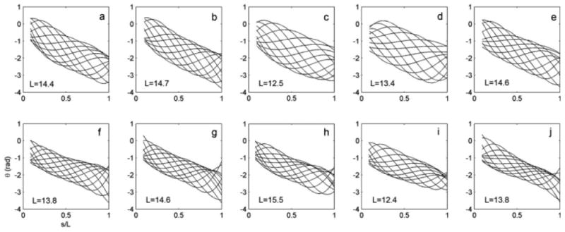
Shear angle plots are shown at intervals of 1/12 cycle, corresponding to the waveforms of Fig. 6. Lengths (μm) are noted on each plot. Plots start at nonzero values of s/L because the flagellum cannot be well resolved within ∼ 1 μm of the proximal end.

Table II. Comparison of Waveform Parameters for Wild-Type and ida3 Chlamydomonas Flagella to Analogous Parameters Obtained by Brokaw and Kamiya (1987) for Wild-Type, ida98 and pf30 Chlamydomonas Flagella.

Parameter	Wild-type	ida3	B and K WT	B and K ida98	B and K pf30
N	12	12	40	37	31
f (Hz)	69.6 ± 8.7	62.5 ± 9.5	63.3 ± 6.3	55.2 ± 7.2	57.2 ± 6.5
L (μm)	13.4 ± 0.9	13.9 ± 1.0	12.8 ± 1.5	10.4 ± 1.2	11.3 ± 1.6
κP (rad/μlm)	0.520 ± 0.052	0.475 ± 0.056	0.62 ± 0.06	0.59 ± 0.04	0.62 ± 0.05
κR (rad/μm)	0.131 ± 0.025	0.122 ± 0.025	0.13 ± 0.04	0.10 ± 0.05	0.10 ± 0.05
VP (rad/cyc)	7.71 ± 0.64	6.95 ± 1.14	6.8 ± 0.8	4.6 ± 0.7	5.4 ± 0.8
VR (rad/cyc)	5.55 ± 0.56	4.22 ± 0.39	4.5 ± 0.6	3.4 ± 0.5	3.3 ± 0.3
τPR (cyc)	0.445 ± 0.023	0.321 ± 0.036	0.36 ± 0.07	0.33 ± 0.08	0.30 ± 0.14

Shear angle represents the cumulative effects of local dynein activity, integrated along the flagellum. Local activity is illuminated by maps of curvature: $\mathrm{\kappa }=\frac{d\mathrm{\theta }}{\mathit{\text{ds}}}$. We normalize curvature by the length of the flagellum, L, so κ has units of rad/flagellar length; we can convert to physical curvature in rad/μm by dividing by L. Figure 8 shows the curvature plots corresponding to the wild-type (a–e) and ida3 waveforms (f–j) of Fig. 6. While each map shows curvatures of similar magnitude, the negative curvature band (corresponding to the primary, or P, bend) is narrower in ida3. This is reinforced by cross-sectional plots of curvature versus time (Figs. 8k–8o) at the midpoint of the flagellum. One other feature becomes apparent if the locations of peak curvature are tracked over a cycle (Fig. 9). The reverse (R) bend starts earlier and propagates more slowly in ida3 than in wild-type Chlamydomonas. These differences in timing and speed of the reverse bend relative to the primary bend appear fundamental to the differences in the ida3 waveform.

Fig. 9. Time-space trajectories of the points of maximum and minimum curvature for the flagellar waveforms of Figs. 6–8.

Top row: wild-type. The average ratio between the propagation speed of the reverse bend (slope of red line, R) and the propagation speed of the principal bend (slope of the blue curve, P) is 1.03 ± 0.09 (N = 12 wild-type cells). Bottom row: ida3. The average ratio between the propagation speed of the reverse bend and the propagation speed of the principal bend is 0.73 ± 0.09 (N = 12 ida3).

These figures are augmented by statistics of this representation of the waveform (Fig. 10). The average values of minimum (and maximum) curvature in the principal and reverse bends, sliding velocity, delay between the initiation of these bends at the proximal end, and the propagation speed of the bends are shown in Table I. It is interesting to note that while the differences in principal and reverse curvature values between wild-type and ida3 are not great, the parameters that describe the relative timing and location of the two bends differ more significantly.

Fig. 10. Statistical comparison of the uni1 wild-type and ida3 flagellar waveforms.

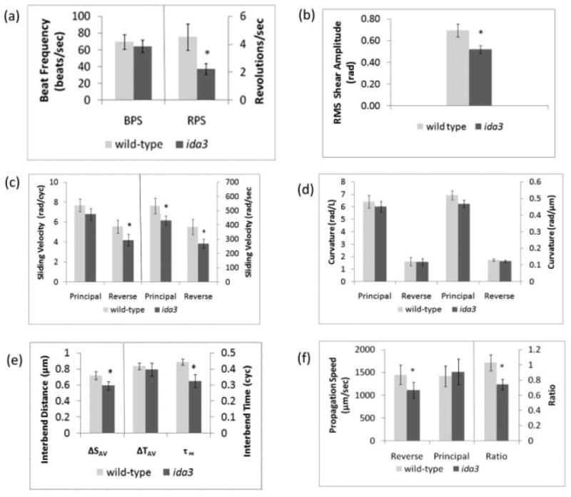
(a) Beat frequency (BPS = beats/s) and rotation rate (RPS = revs/s). (b) The average root-mean-square (RMS) amplitude of shear angle variation. (c) Sliding velocity measured in both nondimensional (rad/cyc) and physical units (rad/s). (d) Average values of the principal bend curvature and reverse bend curvature measured in both nondimensional (rad/length) and physical units (rad/μm). (e) Spatial and temporal measures of coordination between bends. The mean inter-bend distance ΔS_AV represents the average normalized distance between the points of minimum (principal) and maximum (reverse) curvature. The mean inter-bend time ΔT_AV represents the average time between the occurrence of the minimum (principal) and maximum (reverse) curvatures. The time delay τ_PR represents the delay between the initiation of the principal and the reverse bend. (f) Propagation speeds of the principal and reverse bends, and the ratio of propagation speeds (reverse/principal). In all summary plots, averages are computed over all time points and all locations in the middle 80% of the flagellum, and include all wild-type or ida3 cells.

In Table II we compare waveform parameters obtained by the current approach to the approximately analogous parameters obtained by Brokaw and Kamiya [1987] for wild-type Chlamydomonas and two inner-arm mutants: ida98 and pf30. These are alleles at the ida1 locus that affect the I1 inner dynein arm to produce phenotypic behavior similiar to ida3 strains. Brokaw and Kamiya [1987] use piece-wise constant-curvature fitting of stroboscopically obtained flagellar images to obtain their waveform parameters. Values of curvature, sliding velocity, and bend initiation delay are quantitatively similar, in the two studies. The two approaches detect generally similar differences between principal and reverse bends and between wild-type and mutant waveforms. The current study generated slightly lower curvature values and slightly higher sliding velocities compared to the prior study. Two basic parameters of the flagellar motion, independent of the analysis method, appear to be different in the two studies. The beat frequencies in Brokaw and Kamiya [1987] are slower (Table II) and the flagellar lengths are shorter than those in the current study. These may be due to differences in culture conditions. Brokaw and Kamiya [1987] use gametic cells, while vegetatively growing cells are used in this study. The calculated values of curvature and sliding velocity in the two studies are affected by length and beat frequency. Longer flagella of comparable shape will have lower curvature, and faster-beating flagella of comparable shape will have higher sliding velocity. We conclude that given these differences in the experimental model, the results of the current method are in generally good agreement with the prior work of Brokaw and colleagues.

Discussion

Understanding of the generation of waveforms in eukaryotic cilia and flagella is still rudimentary. The doublets slide relative to the neighbor towards the distal end by the coordinated action of dynein arms. However, how the sliding is converted to a waveform and the role of the structural and physical properties of the flagella are not well documented. One way to gain parameters for modeling the waveforms is to use mutants and drugs that perturb the action of the dynein arms and other flagellar structures and compare the waveform generated to waveforms from untreated cells. We present a method for acquiring this type of data on wild-type and mutant or treated cells. Our approach provides excellent spatial and temporal resolution with which to analyze and describe the Chlamydomonas waveform. In this work, we have analyzed the ida3 mutant strain, which lacks the I1 inner dynein arm [Kamiya et al., 1991], as a representative of this approach. The I1 dynein is involved in the regulation of flagellar waveform [Brokaw and Kamiya, 1987]. However to date, the ida3 gene has not been identified. It is unlikely that the ida3 gene encodes a structural component of the I1 dynein arm as none of these genes for structural proteins map to the same genetic interval as ida3 on linkage group III [Wirschell et al., 2009].

High spatiotemporal resolution is obtained by taking advantage of recently developed mathematical tools. Analysis of the flagellar waveform is challenging in general because the flagellum represents a tiny fraction of the image, and this small component is constantly moving throughout the field of view. Furthermore, obtaining adequate temporal resolution with standard laboratory cameras, even “high-speed” (100–350 frames/s) is difficult. The temporal sampling rate used in this study (350 frames/s) is sufficient to characterize the gross behavior of an oscillating flagellum beating at 60–70 frames/s, but without additional steps such as those used in this study, the resolution (about 5–6 frames/cycle) is inadequate for describing the details of wave motion.

A key step, the nonlinear dimension reduction and sorting scheme, Isomap [Tenenbaum et al., 2000] provides high effective temporal resolution by sorting data from multiple cycles to form a single representative cycle. This approach would fail if the beat frequency were a constant integer ratio of the sampling frequency, since the entire cycle would not be sampled. However, in practice, this is unlikely to occur, especially as the beat frequency varies slightly in time. Sorting ensures that the parameters from the curve-fit to one flagellar point cloud are good initial estimates for the parameters of the next fit. This greatly improves the efficiency of the fitting procedure and reduces the risk that the minimization algorithm might find a spurious local minimum of the objective function. In addition, sorting allows the user to smooth results temporally, since the physical variation of the waveform in time is smooth. The disadvantage of sorting is that the accuracy of the final representation rests on the two assumptions of periodicity and approximately regular sampling. If these are violated, then the analysis is invalid.

A second key algorithm is the automatic measurement and subtraction of rigid-body motion, so that the flagellum is described with respect to a fixed origin at its base. This allows successful registration of flagellar point clouds to a common origin, and simultaneously provides estimates of the rotation and beat frequency.

Current high-speed video camera technology allows us to capture movements at 350 frames per second with 320 × 240 pixel frames. These frame rates are necessary to capture flagellar motion, but generate enormous data sets. Without automated methods such as those described here, flagellar waveform analysis would be prohibitively labor-intensive. However, automated methods can only be successful if video images have sufficient contrast so that the pixels on the flagellum can be identified reliably. The “halo” around the body prevents accurate characterization of the most proximal 1 μm section, and pixel identification is less reliable as contrast drops off at the distal tip. Accordingly, the curve fit is probably least accurate at the proximal and distal extremes. Alternative methods for identification of flagellar pixels may be used, as long as the resulting point clouds accurately represent the shape at each time.

As in the studies of Brokaw [Brokaw et al., 1982; Huang et al., 1982; Brokaw and Luck, 1983; Brokaw, 1984; Brokaw and Kamiya, 1987], we have used the uni1 mutant strain, which assembles only one flagellum in most cells. The assembled flagellum is found trans to the eyespot [Huang et al., 1982] and is assembled on the older basal body [Holmes and Dutcher, 1989]. If there are differences between the trans and cis flagellar waveforms, this method will not detect these differences. The properties of the flagellar waveforms from wild-type cells are in generally good agreement with previously gathered data [Brokaw et al., 1982; Huang et al., 1982; Brokaw, 1983, 1984; Brokaw and Kamiya, 1987]. In addition, the differences in waveform characteristic of the ida3 mutant are similar to those seen by Brokaw and Kamiya [1987] in ida1 alleles (ida98 and pf30). It should be noted that, although ida3 and the mutants in the prior study all lack the I1 inner dynein arm, the ida3 gene has yet to be precisely mapped and identified and could differ from other I1 mutants. Also small systematic differences in corresponding parameters between wild-type Chlamydomonas in the current study and Brokaw's earlier work may reflect subtle differences in the cell physiology of gametic and vegetative cells, as well as differences in the estimation methods.

Wild-type and ida3 cells show similar beat frequencies, and similar maximum and minimum curvature when normalized by flagellar length and cycle time (Table I). Other waveform parameters are significantly different between wild-type and ida3 data. These include the root-mean-square (RMS) amplitude of shear angle (calculated over the middle 80% of the flagellum), as well as the propagation speeds of principal and reverse bends (Table I, Figs. 8–10). These observations suggest that the timing of dynein activity in ida3 cells leads to shorter recovery and power strokes. In other words, the reverse bend begins earlier and travels more slowly relative to the principal bend, than in wild-type cells. Some biophysical feature of the ida3 mutant, likely associated with loss of the I1 dynein arm, appears to change the timing of dynein activity.

As well as clarifying differences in axonemal shape, the path of the flagellum through space and time describes a velocity field. The components of velocity in Cartesian coordinates can be obtained for every point on the flagellum (Fig. 11), by simple numerical differentiation of the x(s, t) and y(s, t) fields with respect to time. The smooth, well resolved descriptions of the flagellum in space and time obtained by the current method allow accurate estimation of velocities. We present this only as a preliminary example of further biophysical analyses that can be performed. For instance, drag force on the flagellum can be calculated as a function of space and time, and integrated to provide estimates of net propulsive force and power. These parameters can be studied in media of different viscosity (for example) to investigate how mutations or interventions affect behavior under different loading conditions.

Fig. 11. Velocity vectors at selected points on the flagellum at 12 equally-spaced times in the flagellar cycle (wild-type).

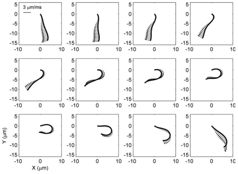
The enhanced spatial and temporal resolution provided by the current algorithm enables accurate estimation of velocity field. Other mechanical parameters, such as propulsive force and power can be estimated from the velocity field.

In biflagellate Chlamydomonas, flagellar motion is not strictly planar; a small three-dimensional component exists, causing rotation of the cell about its long axis [Rüffer and Nultsch, 1985]. In the uniflagellate cells studied here, the 3D component is probably negligible [Brokaw et al., 1982]. The current analysis is also limited to steady-state periodic motion. The technique might be extended to study transient behavior, such as a phototactic response [Rüffer and Nultsch, 1990, 1991; Harz and Hegemann, 1991], under a protocol that consistently produces repeatable stimulus-response behavior. Finally, only uniflagellate cells were characterized in this study. It should be possible to study biflagellate motion if the cell body is captured on a micropipette [as in, for example, Rüffer and Nultsch, 1987, 1990, 1991; Harz and Hegemann, 1991] so that the flagella would remain in the field of view for multiple beats.

Future work will include the application of this method to characterize flagellar behavior in a variety of other mutants. Ultimately, we hope these tools can illuminate the biophysics and genetics of ciliopathies that may be modeled in Chlamydomonas.

References

- Bower R, VanderWaal K, O'Toole E, Fox L, Perrone C, Mueller J, Wirschell M, Kamiya R, Sale WS, Porter ME. IC138 defines a sub-domain at the base of the I1 dynein that regulates microtubule sliding and flagellar motility. Mol Biol Cell. 2009;20:3055–3063. doi: 10.1091/mbc.E09-04-0277. [DOI] [PMC free article] [PubMed] [Google Scholar]
- Brokaw C. Automated methods for estimation of sperm flagellar bending parameters. Cell Motil Cytoskeleton. 1984;4:417–430. doi: 10.1002/cm.970040603. [DOI] [PubMed] [Google Scholar]
- Brokaw C. Control of flagellar bending: a new agenda based on dynein diversity. Cell Motil Cytoskeleton. 1994;28:199–204. doi: 10.1002/cm.970280303. [DOI] [PubMed] [Google Scholar]
- Brokaw C, Kamyia R. Bending patterns of Chlamydomonas flagella IV: mutants with defects in inner and outer dynein arms indicate differences in dynein arm function. Cell Motil Cytoskeleton. 1987;8:68–75. doi: 10.1002/cm.970080110. [DOI] [PubMed] [Google Scholar]
- Brokaw C, Luck D. Bending patterns of Chlamydomonas flagella I: wild-type bending patterns. Cell Motil Cytoskeleton. 1983;3:131–150. doi: 10.1002/cm.970030204. [DOI] [PubMed] [Google Scholar]
- Brokaw C, Luck D. Bending patterns of Chlamydomonas flagella: III. A radial spoke head deficient mutant and a central pair deficient mutant. Cell Motil Cytoskeleton. 1985;5:195–208. doi: 10.1002/cm.970050303. [DOI] [PubMed] [Google Scholar]
- Brokaw C, Luck D, Huang B. Analysis of the movement of Chlamydomonas flagella: the function of the radial-spoke system is revealed by comparison of wild-type and mutant flagella. J Cell Biol. 1982;92:722–732. doi: 10.1083/jcb.92.3.722. [DOI] [PMC free article] [PubMed] [Google Scholar]
- Brokaw CJ. Computerized analysis of flagellar motility by digitization and fitting of film images with straight segments of equal length. Cell Motil Cytoskeleton. 1990;17:309–316. doi: 10.1002/cm.970170406. [DOI] [PubMed] [Google Scholar]
- Dutcher SK. Mating and tetrad analysis in Chlamydomonas reinhardtii. Methods Cell Biol. 1995;47:531–540. doi: 10.1016/s0091-679x(08)60857-2. [DOI] [PubMed] [Google Scholar]
- Dutcher SK, Gibbons W, Inwood WB. A genetic analysis of suppressors of the PF10 Mutation in Chlamydomonas reinhardtii. Genetics. 1988;120:965–976. doi: 10.1093/genetics/120.4.965. [DOI] [PMC free article] [PubMed] [Google Scholar]
- Harz H, Hegemann P. Rhodopsin-regulated calcium currents in Chlamydomonas. Nature. 1991;351:489–491. [Google Scholar]
- Holmes J, Dutcher S. Cellular asymmetry in Chlamydomonas reinhardtii. J Cell Sci. 1989;94:273–285. doi: 10.1242/jcs.94.2.273. [DOI] [PubMed] [Google Scholar]
- Huang B, Ramanis Z, Dutcher SK, Luck DJL. Uniflagellar mutants of chlamydomonas: evidence for the role of basal bodies in transmission of positional information. Cell. 1982;29:745–753. doi: 10.1016/0092-8674(82)90436-6. [DOI] [PubMed] [Google Scholar]
- Kamiya R, Kurimoto E, Muto E. Two types of Chlamydomonas flagellar mutants missing different components of inner-arm dynein. J Cell Biol. 1991;112:441–447. doi: 10.1083/jcb.112.3.441. [DOI] [PMC free article] [PubMed] [Google Scholar]
- King SJ, Dutcher SK. Phosphoregulation of an inner dynein arm complex in Chlamydomonas reinhardtii is altered in phototactic mutant strains. J Cell Biol. 1997;136:177–191. doi: 10.1083/jcb.136.1.177. [DOI] [PMC free article] [PubMed] [Google Scholar]
- King SJ, Inwood WB, O'Toole ET, Power J, Dutcher SK. The bop2– 1 mutation reveals radial asymmetry in the inner dynein arm region of Chlamydomonas reinhardtii. J Cell Biol. 1994;126:1255–1266. doi: 10.1083/jcb.126.5.1255. [DOI] [PMC free article] [PubMed] [Google Scholar]
- King SM, Kamiya R. Axonemal dyneins: assembly, structure and force generation. In: Witman GB, editor. The Chlamydomonas Sourcebook. 2nd. San Diego: Academic Press; 2008. pp. 131–208. [Google Scholar]
- Lux FG, 3rd, Dutcher SK. Genetic interactions at the FLA10 locus: suppressors and synthetic phenotypes that affect the cell cycle and flagellar function in Chlamydomonas reinhardtii. Genetics. 1991;128:549–561. doi: 10.1093/genetics/128.3.549. [DOI] [PMC free article] [PubMed] [Google Scholar]
- Nicastro D, Schwartz C, Pierson J, Gaudette R, Porter ME, McIntosh JR. The molecular architecture of axonemes revealed by cryoelectron tomography. Science. 2006;313:944–948. doi: 10.1126/science.1128618. [DOI] [PubMed] [Google Scholar]
- Okita N, Isogai N, Hirono M, Kamiya R, Yoshimura K. Phototactic activity in Chlamydomonas ‘non-phototactic’ mutants deficient in Ca2+-dependent control of flagellar dominance or in inner-arm dynein. J Cell Sci. 2005;118:529–537. doi: 10.1242/jcs.01633. [DOI] [PubMed] [Google Scholar]
- Piperno G, Ramanis Z, Smith E, Sale W. Three distinct inner dynein arms in Chlamydomonas flagella: molecular composition and location in the axoneme. J Cell Biol. 1990;110:379–389. doi: 10.1083/jcb.110.2.379. [DOI] [PMC free article] [PubMed] [Google Scholar]
- Pless RB. Image spaces and video trajectories: using isomap to explore video sequences. Proc IEEE Int Conf Comput Vis. 2003;2:1433–1440. [Google Scholar]
- Pless RB, Simon I. Conference on Imaging Science Systems and Technology. Athens, GA: CSREA Press; 2002. Embedding images in non-flat spaces; pp. 182–188. [Google Scholar]
- Porter M, Power J, Dutcher S. Extragenic suppressors of paralyzed flagellar mutations in Chlamydomonas reinhardtii identify loci that alter the inner dynein arms. J Cell Biol. 1992;118:1163–1176. doi: 10.1083/jcb.118.5.1163. [DOI] [PMC free article] [PubMed] [Google Scholar]
- Porter ME, Sale WS. The 9 + 2 axoneme anchors multiple inner arm dyneins and a network of kinases and phosphatases that control motility. J Cell Biol. 2000;151:37F–42F. doi: 10.1083/jcb.151.5.f37. [DOI] [PMC free article] [PubMed] [Google Scholar]
- Rosenfeld A, Avinash KAK. Digital Picture Processing. New York: Academic Press; 1976. p. 457. [Google Scholar]
- Rüffer U, Nultsch W. High speed cinematographic analysis of the movement of Chlamydomonas. Cell Motil Cytoskeleton. 1985;5:251–263. [Google Scholar]
- Rüffer U, Nultsch W. Comparison of the beating of cis- and trans-flagella of Chlamydomonas cells held on micropipettes. Cell Motil Cytoskeleton. 1987;7:87–93. doi: 10.1002/(SICI)1097-0169(1998)41:4<297::AID-CM3>3.0.CO;2-Y. [DOI] [PubMed] [Google Scholar]
- Rüffer U, Nultsch W. Flagellar photoresponses of Chlamydomonas cells held on micropipettes: I. Changes in flagellar beat frequency. Cell Motil Cytoskeleton. 1990;15:162–167. [Google Scholar]
- Rüffer U, Nultsch W. Flagellar photoresponses of Chlamydomonas cells held on micropipettes: II. Changes in flagellar beat pattern. Cell Motil Cytoskeleton. 1991;18:269–278. [Google Scholar]
- Smith EF, Yang P. The radial spokes and central apparatus: mechanochemical transducers that regulate flagellar motility. Cell Motil Cytoskeleton. 2004;57:8–17. doi: 10.1002/cm.10155. [DOI] [PMC free article] [PubMed] [Google Scholar]
- Summers KE, Gibbons IR. Adenosine triphosphate-induced sliding of tubules in trypsin-treated flagella of sea-urchin sperm. Proc Natl Acad Sci USA. 1971;68:3092–3096. doi: 10.1073/pnas.68.12.3092. [DOI] [PMC free article] [PubMed] [Google Scholar]
- Tenenbaum JB, de Silva V, Langford JC. A global geometric framework for nonlinear dimensionality reduction. Science. 2000;290:2319–2323. doi: 10.1126/science.290.5500.2319. [DOI] [PubMed] [Google Scholar]
- Wirschell M, Sale WS. Keeping an eye on I1: I1 dynein as a model for flagellar dynein assembly and regulation. Cell Motil Cytoskeleton. 2007;64:569–579. doi: 10.1002/cm.20211. [DOI] [PubMed] [Google Scholar]
- Wirschell M, Yang C, Yang P, Fox L, Yanagisawa HA, Kamiya R, Witman GB, Porter ME, Sale WS. IC97 is a novel intermediate chain of I1 dynein that interacts with tubulin and regulates interdoublet sliding. Mol Biol Cell. 2009;20:3044–3054. doi: 10.1091/mbc.E09-04-0276. [DOI] [PMC free article] [PubMed] [Google Scholar]