Basilar-membrane interference patterns from multiple internal reflection of cochlear traveling waves

Abstract

At low stimulus levels, basilar-membrane (BM) mechanical transfer functions in sensitive cochleae manifest a quasiperiodic rippling pattern in both amplitude and phase. Analysis of the responses of active cochlear models suggests that the rippling is a mechanical interference pattern created by multiple internal reflection within the cochlea. In models, the interference arises when reverse-traveling waves responsible for stimulus-frequency otoacoustic emissions (SFOAEs) reflect off the stapes on their way to the ear canal, launching a secondary forward-traveling wave that combines with the primary wave produced by the stimulus. Frequency-dependent phase differences between the two waves then create the rippling pattern measurable on the BM. Measurements of BM ripples and SFOAEs in individual chinchilla ears demonstrate that the ripples are strongly correlated with the acoustic interference pattern measured in ear-canal pressure, consistent with a common origin involving the generation of SFOAEs. In BM responses to clicks, the ripples appear as temporal fine structure in the response envelope (multiple lobes, waxing and waning). Analysis of the ripple spacing and response phase gradients provides a test for the role of fast- and slow-wave modes of reverse energy propagation within the cochlea. The data indicate that SFOAE delays are consistent with reverse slow-wave propagation but much too long to be explained by fast waves.

I. INTRODUCTION

At sound levels near the threshold of hearing, basilar-membrane mechanical transfer functions in highly sensitive, mammalian ears can exhibit a striking, quasiperiodic rippling pattern. Figure 1, for example, shows basilar-membrane (BM) measurements from one of the most mechanically sensitive chinchilla ears studied to date (Rhode, 2007). The asterisks mark spectral ripples evident in both the magnitude and the phase of the transfer function; they appear most prominent at frequencies at and below the characteristic frequency (CF) of the measurement site. Fourier analysis indicates that quasiperiodic ripples in the spectral domain generally appear as temporal bursts, or echoes, in the time domain. Interestingly, complex features—such as multiple lobes and waxing and waning of the response envelope—are regularly seen in BM and auditory-nerve click responses (Recio et al., 1998; Lin and Guinan, 2000; Rhode, 2007; Guinan and Cooper, 2008). These puzzling temporal features have been variously ascribed to “obscure” nonlinear processes (Recio et al., 1998), to beating between multiple vibrational modes in the organ of Corti (Lin and Guinan, 2000, 2004), and to interactions among coupled nonlinear oscillators contributing to the BM impedance (Zweig, 2003; Aranyosi, 2006). Despite the wealth of intriguing hypotheses, the origin and significance of the BM spectral ripples and the complex temporal ringing of the click response remain unclear.

FIG. 1.

Basilar-membrane mechanical transfer functions in a sensitive chinchilla (Rhode, 2007). Iso-intensity transfer functions are shown at stimulus levels of 5–95 dB SPL in 5 dB steps ($\text{CF}\hspace{0.17em}\hspace{0.17em}\cong$ 9.1 kHz). Asterisks mark peaks in the rippling pattern that emerge at low sound levels. The phase curves have been detrended by subtracting a constant delay (0.69 ms) whose presence would otherwise obscure the ripples. At the highest levels, another rippling pattern, different from that discussed here, appears at frequencies above CF. Adapted from Figs. 2 and 4 of Rhode (2007).

Here we develop and test an alternative hypothesis to explain the BM spectral ripples and their time-domain counterparts, namely, that they arise from wave interference effects related to the generation of otoacoustic emissions (Shera, 2001a; de Boer and Nuttall, 2006; Shera and Cooper, 2009). Spectral interference patterns created by the alternating constructive and destructive superposition of waves originating from different sources are common in otoacoustic measurements. The rippling pattern known as distortion-product fine structure, for example, results from the interference between emission components whose relative phase rotates regularly with frequency, reflecting their different mechanisms of generation within the cochlea (e.g., Talmadge et al., 1998; Shera and Guinan, 1999; Kalluri and Shera, 2001). Stimulus-frequency otoacoustic emissions provide another example, in which the delayed emission sums with the evoking tone to create an oscillatory pattern in the total ear-canal pressure (e.g., Kemp and Chum, 1980; Zwicker and Schloth, 1984; Shera and Zweig, 1993). Models indicate that the fluids and structures of the inner ear support bidirectional wave propagation and reflection and predict that interference patterns of otoacoustic origin should appear not only in the ear canal but also within the cochlea (Shera and Zweig, 1992). Indeed, the quasiperiodic microstructure of the hearing threshold curve (e.g., Elliot, 1958; Thomas, 1975) provides compelling psychophysical evidence that something resembling standing-wave interference modulates the firing patterns of the auditory nerve (Long, 1984; Kemp, 2002).

We hypothesize that the BM rippling patterns evident in Fig. 1 and elsewhere arise as OAE-related mechanical interference patterns in basilar-membrane motion. Although the decrease in ripple amplitude with increasing stimulus intensity appears consistent with the compressive growth expected from stimulus-frequency otoacoustic emissions, no emissions were measured in the study and so the relationship, if any, between the BM ripples and otoacoustic emissions remains unclear. Here, we combine mechanical and otoacoustic measurements to test model-based hypotheses about the origin of the BM ripples. We demonstrate using measurements of BM motion and OAEs from the same ears that the mechanical and otoacoustic interference patterns are strongly correlated, consistent with a common origin involving stimulus-frequency emissions. Although ripples in BM motion are of intrinsic interest as mechanical analogs of threshold microstructure, their association with evoked otoacoustic emissions also provides a tool for exploring modes of energy propagation within the cochlea. Developing this idea, we analyze our measurements to test the otoacoustic and BM rippling patterns for consistency with predictions of the so-called “slow-” and “fast-wave” models of reverse propagation.

II. MULTIPLE INTERNAL REFLECTION OF OTOACOUSTIC ENERGY

We hypothesize that BM ripples represent an interference pattern created by multiple internal reflection within the cochlea. Figure 2 illustrates the idea. Reverse pressure waves created by coherent wave scattering (or, more generally, by the “stimulated emission”) of a primary forward-traveling wave within the cochlea partially reflect off the boundary with the middle ear on their way to the ear canal. This reflection launches a secondary forward-traveling wave that combines with the primary wave produced by the stimulus. Frequency-dependent phase differences between the two forward-traveling waves then create the quasiperiodic rippling pattern measurable on the BM. An analogous interference between multiple waves occurs in the ear canal. Reverse traveling energy unreflected at the stapes travels through the middle ear to the ear canal, where it appears as an otoacoustic emission at the stimulus frequency (an SFOAE). In the ear canal, the emission sums with the stimulus to produce the characteristic acoustic interference pattern seen in the total ear-canal pressure in response to a swept tone.

FIG. 2.

Wave reflection mechanisms hypothesized to produce interference ripples in both ear-canal pressure and BM motion. The distributed process of wave scattering produces multiple wavelets that combine to form a net reverse wave that is then partially reflected at the stapes and partially transmitted to the ear canal.

A. A model realization

We gave substance to our hypothesis and made quantitative predictions about the effects of multiple internal reflection using an active model of the cochlea (Zweig, 1991). To generate reflection-source otoacoustic emissions (SFOAEs), we augmented the basic model with micromechanical irregularities in the BM admittance, as suggested by coherent reflection theory (Zweig and Shera, 1995). The spatial irregularity was introduced by randomly jittering the poles of the BM admittance by a few percent in the complex frequency plane. This has the effect of producing small, irregular spatial variations in the gain of the cochlear amplifier. To simulate the dependence on stimulus intensity, we employed a series of linear models differing in their overall amplifier gain. The gain was varied by moving the poles of the BM admittance along lines perpendicular to the real frequency axis (Shera, 2001b). Model responses were computed numerically using finite differences.¹

Figure 3 shows model BM transfer functions and ear-canal pressures normalized by stimulus amplitude. BM ripples resembling those seen in the animal data of Fig. 1 are clearly evident in the model responses (top).² Although not shown here, corresponding oscillations are seen in the model phase. As in the animal data, the ripple amplitude appears largest at low stimulus levels; at higher levels, the ripples decrease and eventually become undetectable. As suggested by the mechanisms portrayed in Fig. 2, the model predicts that the BM rippling pattern is strongly correlated with the ripples in ear-canal pressure produced by SFOAEs (bottom).

FIG. 3.

Interference patterns in BM velocity transfer functions and ear-canal pressure computed using an active cochlear model supplemented with mechanical irregularities in the BM admittance. The BM frequency responses were computed at the cochlear location with characteristic frequency of 8.2 kHz. The magnitude of the BM ripples depends on the gain of the cochlear amplifier, the size of the irregularities, and the stapes reflection coefficient; in this example, the amplifier gain was relatively low and $R_{\text{stapes}}$ was set to 0.95. The precise alignment of the BM and ear-canal interference peaks was obtained by adjusting model parameters (e.g., the relative phase of $G_{\text{ME}}^{\rightleftarrows }$ and $R_{\text{stapes}}$) and is not therefore a general prediction of the model.

1. Analytic approximations

The origin of the ripples and their dependence on model parameters can be better appreciated by deriving approximate analytic formulae for the responses shown in Fig. 3. To obtain the BM-velocity traveling wave, $V_{\text{BM}}\left(x,f\right)$, one solves the model equations for the traveling pressure-difference wave, P_BM(x, f ), and multiplies it by the BM admittance: $V_{\text{BM}}\left(x,f\right)=Y_{\text{BM}}\left(x,f\right)P_{\text{BM}}\left(x,f\right)$. We obtain an approximate expression for P_BM(x, f ) in the presence of mechanical irregularities using traveling-wave Green's functions and the Born scattering series (Shera et al., 2005). To first order in the irregularities, the transpartition pressure has the form³

$$\begin{array}{c}{P}_{\text{BM}}(x)\cong P_{\mathrm{S}}{G}_{\text{ME}}^{\to }\{W_r(x)\left[1+\underset{\mathit{A}}{\underbrace{\gamma R_{\text{stapes}}{\displaystyle {\int }_0^L\varrho W_r^{2}d{x}^{\prime }}}}+\underset{\mathit{B}}{\underbrace{\gamma {\displaystyle {\int }_0^x\varrho W_r{W}_{l}d{x}^{\prime }}}}\right]+W_l(x)\left[\underset{\mathit{C}}{\underbrace{\gamma {\displaystyle {\int }_x^L\varrho W_r^{2}d{x}^{\prime }}}}\right]\},\end{array}$$ (1)

where, for simplicity, only the x dependence appears explicitly; all quantities are understood to depend on the stimulus frequency, f, and all functions appearing under the integral signs also depend on position. The notation is adopted from Shera et al. (2005). In brief, x is the distance from the stapes, P_S is the ear-canal stimulus pressure, $G_{\text{ME}}^{\to }$ is the forward middle-ear pressure transfer function, $W_{r,l}(x)$ are the traveling pressure basis waves describing right and left (i.e., forward and reverse) wave propagation and amplification along the BM, the dimensionless function $\varrho (x)$ characterizes the micromechanical irregularities that scatter the waves, γ is a constant (the so-called Wronskian determinant), L is the length of the cochlea, and $R_{\text{stapes}}$ is the reflection coefficient for retrograde waves at the stapes (Shera and Zweig, 1991). The traveling pressure basis waves $W_{r,l}(x)$ are both normalized to unity at x = 0; they depend on cochlear geometry and the impedance of the partition, which jointly determine the power gain and wavelength of the traveling wave.

The initial term on the right-hand side of Eq. (1) for P_BM(x)—namely, P_S$G_{\text{ME}}^{\to }$W_r(x) times the 1 in the first set of brackets—represents what the pressure would be if $\varrho$ were zero and there were no mechanical irregularity along the organ of Corti: an unperturbed, forward-traveling wave. The three remaining terms (labeled A, B, and C) arise from wave scattering and modify the form of the pressure. The factor W_l(x) on the second line represents a reverse traveling wave whose amplitude at location x is determined by term C. The integration over x′ in C sums reverse waves originating at all locations apical to the site of measurement (x′ > x). Reverse waves originating at more basal locations (x′ < x) do not contribute to the pressure at x unless they reflect at the stapes and propagate to x as a forward wave. Term A represents the summed contribution of all such waves scattered throughout the cochlea and subsequently reflected from the stapes. Finally, term B describes how the amplitude of the forward wave itself is modified by scattering. As indicated by the limits of integration, this term depends on irregularities the wave encounters as it travels from 0 to x.

The integral appearing in term A of Eq. (1) represents the first-order (Born) approximation to the cochlear reflectance, R, defined as the ratio of the outgoing (i.e., reflected) wave to the ingoing (i.e., stimulus) wave at the stapes (e.g., Zweig and Shera, 1995; Shera et al., 2005). When rewritten using the Born approximation for the cochlear reflectance,

$$R\cong \gamma {\displaystyle {\int }_0^L\varrho W_r^2\hspace{0.17em}d{x}^{\prime },}$$ (2)

term A becomes simply $R{R}_{\text{stapes}}$. Because of the form of the basis waves $W_{r,l}(x)$—in particular, the fact that $\left|W_l\right|\ll \left|W_r\right|$ near the peak of the traveling wave [see Fig. 16 and Appendix A of Shera et al. (2005)]—Eq. (1) indicates that the dominant contribution to the BM ripples at frequencies near CF originates in term A. Using this approximation and neglecting terms B and C yields the simplified expression

$$P_{\text{BM}}(x)\cong P_{\mathrm{S}}{G}_{\text{ME}}^{\to }{W}_r(x)\hspace{0.17em}\hspace{0.17em}[1+R\hspace{0.17em}{R}_{\text{stapes}}].$$ (3)

Equation (3) can now be used to approximate the BM rippling pattern by evaluating P_BM(x) at a particular cochlear location, x₁; multiplying by the corresponding BM admittance, $Y_{\text{BM}}(x_1)$, to obtain the local BM velocity, $V_{\text{BM}}(x_1)$; and then repeating the process as a function of frequency. The approximation used in Eq. (3) is valid primarily within the peak region of the traveling wave. Within that region, Eq. (3) indicates that the response is dominated by a forward-traveling wave [since terms in Eq. (1) proportional to $W_l(x)$ are small and have been ignored]. Although not itself large in the peak region, the reverse wave does affect the response when it subsequently reflects from the stapes, combines with the original forward wave, and modifies the total wave amplitude through the term $R{R}_{\text{stapes}}$.

The scattering series can also be used to find the corresponding pressure in the ear canal, $P_{\text{EC}}$. To first order in $\varrho$,

$$P_{\text{EC}}\cong P_{\mathrm{S}}\left[1+G_{\text{ME}}^{\rightleftarrows }\underset{A+C\hspace{0.17em}\text{at}\hspace{0.17em}x=0}{\underbrace{\gamma (1+R_{\text{stapes}}){\displaystyle {\int }_0^L\varrho W_r^{2}d{x}^{\prime }}}}\right],$$ (4)

where we have used the normalization $W_{r,l}$(0) = 1 (Shera et al., 2005). Once again, we have omitted the explicit frequency dependence. The new factor in Eq. (4), $G_{\text{ME}}^{\rightleftarrows }$, describes roundtrip transmission through the middle ear.⁴ The first term on the right, $P_{\mathrm{S}}\times 1$, is just the applied stimulus pressure. The second term gives the pressure due to the emission, $P_{\text{SFOAE}}$; it corresponds to the sum of terms A and C from Eq. (1), evaluated at the stapes (x = 0), and then transmitted through the middle ear. Term B from Eq. (1) is zero at x = 0 and therefore does not contribute. Written using the cochlear reflectance, the emission pressure has the form

$$P_{\text{SFOAE}}\cong P_{\mathrm{S}}{G}_{\text{ME}}^{\rightleftarrows }(1+R_{\text{stapes}})\hspace{0.17em}R,$$ (5)

and the total ear-canal pressure $(P_{\mathrm{S}}+P_{\text{SFOAE}})$ becomes

$$P_{\text{EC}}\cong P_{\mathrm{S}}\hspace{0.17em}[1+G_{\text{ME}}^{\rightleftarrows }(1+R_{\text{stapes}})\hspace{0.17em}R].$$ (6)

2. Origin of the rippling patterns

To understand the common origin of the interference patterns in BM motion and ear-canal pressure, recall that, empirically, SFOAE phase rotates rapidly with frequency (e.g., Kemp and Chum, 1980; Shera and Guinan, 1999). Coherent-reflection theory indicates that this strong frequency dependence originates almost entirely in the cochlear reflectance, R, as a consequence of the breaking of scaling symmetry by the “place-fixed” nature of the mechanical irregularities (Zweig and Shera, 1995). [The phases of the other quantities in Eq. (5) are dominated by middle-ear mechanics and vary relatively slowly with frequency.] According to Eqs. (3) and (6), the rippling patterns seen in both BM velocity and ear-canal pressure are therefore strongly correlated—both patterns arise because their equations contain terms proportional to R, whose phase rotates quasiperiodically with frequency. These terms add alternately in and out of phase with the primary pressures, which are represented in both equations by the constant “1” inside the brackets and the common factors outside that multiply it.

Although both the ear-canal and BM ripples in the model trace their origin to the form of the cochlear reflectance, R—and thus to wave reflection inside the cochlea—specific features of the two rippling patterns (e.g., their amplitudes and phases at any given frequency) are not necessarily identical. Whereas the BM ripples depend on the value of $R{R}_{\text{stapes}}$, the SFOAEs and related ear-canal ripples depend on $G_{\text{ME}}^{\rightleftarrows }\hspace{0.17em}(1+R_{\text{stapes}})$R [cf. Eqs. (3) and (6)]. As indicated, both expressions are proportional to R, but they depend differently on middle-ear transmission and reflection coefficients. For example, the BM ripples disappear in the limit that $R_{\text{stapes}}$ → 0, but in the same limit, all other things being equal,⁵ the ear-canal ripples remain prominent and approach the finite value $G_{\text{ME}}^{\rightleftarrows }$R. Measurements indicate that middle-ear transfer functions and cochlear input and output impedances can manifest significant intersubject variability (Songer and Rosowski, 2007; Ravicz et al., 2010; Ravicz and Rosowski, 2012). Thus, although the model predicts strong correlations between the two rippling patterns whenever they appear, their relative prominence in any given frequency range is likely to vary from animal to animal.

3. Dependence on model parameters

To test the validity of the analysis and approximations underlying Eqs. (1)–(6) while illustrating the process of multiple internal reflection, we used the computational model to explore the dependence of the interference ripples on key model parameters. As expected, the magnitude of the ripples depends on variables such as the gain of the cochlear amplifier [i.e., on the basis waves $W_{r,l}(x)$, whose form varies with stimulus intensity in our series of linear models], on the size and distribution of mechanical irregularities [i.e., on $\varrho \hspace{0.17em}(x)$], and on the amount of reflection that occurs at the stapes [$R_{\text{stapes}}$]. We expect all of these quantities—or their in vivo analogs—to vary from animal to animal. Figure 4, for example, shows that the model BM ripples decrease substantially when the stapes reflection coefficient is reduced (in this case, set to zero) by appropriately modifying the impedance of the middle ear (top panel). The decrease in ripple amplitude is especially pronounced near the peak of the transfer function, as predicted from the relative amplitudes of the basis waves. Some small ripples remain because setting $R_{\text{stapes}}$ to zero affects neither the reverse-traveling wave nor its interference with the forward wave [i.e., terms B and C in Eq. (3) remain nonzero]. By contrast, the ripples disappear completely when the micromechanical irregularities responsible for scattering the forward-traveling wave are removed (bottom panel). Different animals can be simulated by using different sets of irregularities and different values of $R_{\text{stapes}}$. Although details of the ear-canal and BM rippling patterns (e.g., the variation in their amplitude across frequency) depend on the particular set of irregularities used in the model, both patterns depend on the irregularities through the common factor of R, and the correlation between the two patterns is therefore unaffected.

FIG. 4.

Low-level BM ripples depend on multiple internal reflection in the model. The three panels show how wave interference patterns depend on parameters that control the degree of internal reflection in the model. The top panel reproduces the transfer function magnitudes from Fig. 3. The middle panel shows model transfer functions computed using $R_{\text{stapes}}$ = 0; the bottom panel shows the results obtained using $\varrho (x)=0$.

III. TESTING THE REFLECTION HYPOTHESIS

We tested model predictions in chinchilla by measuring BM vibrations and SFOAEs in the same ears.

A. Methods

Measurements were made on deeply anesthetized chinchillas in accordance with NIH, UK, and US guidelines. Intra-peritoneal injections of pentobarbital sodium were administered at an initial dose of 75 mg/kg body weight. The subsequent depth of anesthesia was monitored at regular intervals (typically every 30 min, but more often when needed) and top-up doses of between 15 and 30 mg/kg of sodium pentobarbital were administered as required to abolish all signs of reflex activity in response to a strong toe-pinch (pinch-evoked changes in ECG rate typically proved to be much more sensitive indicators of reflex activity than the voluntary muscle withdrawal-type reflexes used in many studies). Long-term recordings of the animal's ECG covaried reliably with the observed depth of the anesthesia.

Basilar membrane and ossicular vibrations were recorded in one ear of each animal using a displacement-sensitive laser interferometer and well documented procedures (Cooper, 1999). Briefly, the BM was exposed by shaving a small hole into the scala tympani. Gold-coated polystyrene or silver-coated hollow glass microbeads (15–25 μm diameter), and in one experiment stainless steel beads, were dropped through the fluid onto the BM to enhance the reflectivity of the interferometer's incident laser beam (see the Appendix). A small glass cover slip was placed over the cochlear hole to eliminate a mobile air-fluid interface that can create interferometric artifacts (Cooper and Rhode, 1992). Acoustic stimuli were produced using reverse-driven Brüel and Kjaer $\frac{1}{2}$-in. microphones and delivered to the ear canal via a closed sound system. Tone amplitudes were calibrated in the ear canal using a microphone (Brüel and Kjaer 4134) equipped with a probe tube inserted to within 2 mm of the tympanic membrane. SFOAEs were measured using the suppression paradigm (Shera and Guinan, 1999); comparisons in humans indicate that the different SFOAE measurement paradigms (suppression, compression, spectral smoothing) all yield equivalent results (Kalluri and Shera, 2007). Probe frequencies were typically varied from 2–10 kHz in 0.2 kHz steps at levels of 20, 30, and/or 40 dB sound pressure level (SPL); the suppressor tone was always 100 Hz above the probe and 15 dB higher in level. Emissions were measured both before and after measuring the BM and ossicular vibrations. In general, we found the SFOAEs were little affected by the BM exposure and recording procedures (Cooper and Shera, 2004). Compound action potential (CAP) audiograms were also routinely measured and used to check that cochlear deterioration remained minimal; threshold changes were less than 10 dB in every animal except KCH30. Basilar-membrane transfer functions were derived by normalizing BM frequency responses measured at a wide range of sound levels (e.g., 0–80 dB SPL in 10 dB steps) by the frequency response of the incus measured at high levels (e.g., 70 dB SPL). High sound levels were used to measure middle-ear motion because signal-to-noise ratios (SNRs) are much lower for the incus than for the BM at frequencies near CF. Tone frequencies were typically varied in 100 Hz steps from around 4 to 10 kHz, depending on the CF and sound level used. Full details of the recording conditions and a quantitative synopsis of each experiment can be found in the Appendix.

B. Correlated BM and ear-canal rippling patterns

Figure 5 shows BM and otoacoustic measurements from two sensitive chinchilla ears. Although the BM ripples are smaller than those in Rhode's example (see Fig. 1), our data demonstrate that rippling patterns measured on the BM and in ear-canal pressure are strongly correlated across frequency, as predicted by the model. In the examples of Fig. 5, ripple peaks occur at nearly the same frequencies in both the mechanical and otoacoustic measurements (vertical dotted lines). In addition, the amplitudes of both rippling patterns diminish with increasing stimulus intensity, as predicted. The close correspondence of ripple frequencies is unlikely to be mere coincidence. For example, given the frequency resolution of the SFOAE data, the probability that the four ripple peaks in Fig. 5(A), if located at random on the same interval, would fall at the measurement frequencies closest to those indicated by the BM ripples is less than 0.0006 (p = 1/1820). Interestingly, the ear-canal and BM rippling patterns appear comparable to one another in overall amplitude (in dB). Interpreted using the model [Eqs. (3) and (6)], this rough equality implies that at these frequencies $\left|R_{\text{stapes}}/G_{\text{ME}}^{\rightleftarrows }\left(1\hspace{0.17em}+R_{\text{stapes}}\right)\right|$ is of order 1 in these animals.

FIG. 5.

Magnitudes of BM mechanical transfer functions (top) and normalized ear-canal pressures (bottom) measured in two sensitive chinchilla ears. BM data were recorded from −10 dB SPL [panel (A)] or 0 dB SPL [panel (B)] up to 80 dB SPL in 10 dB steps. The transfer functions overlap, indicating linear behavior, at intensities below 10 dB SPL. Ear-canal pressures were measured at 20, 30, and/or 40 dB SPL probe levels and then normalized by the stimulus amplitude. Dotted vertical lines mark the approximate locations of the peaks in ear-canal pressure and show that the ripples in the BM transfer functions and ear-canal pressures are highly correlated.

Figure 6 shows the measurements from another sensitive chinchilla, in which BM measurements were made at two different longitudinal locations. Although the phase of the BM rippling patterns differ at the two locations—peaks in one align roughly with dips in the other—both are strongly correlated with the pattern seen in the ear-canal pressure. For reasons that we assume relate to physiological vulnerability or interanimal differences in middle-ear mechanics, measurable ripples were observed both in the ear canal and on the BM in only nine of the fourteen chinchilla ears that we tested. (Of the remainder, one animal had poor SFOAEs and four had SFOAEs but no discernible BM ripples—see the Appendix for details.) In all nine cases in which both were measured, the two ripple patterns were highly correlated. Our results thus support the multiple-reflection hypothesis and its model realization. The BM and ear-canal rippling patterns appear to share a common origin involving evoked stimulus-frequency emissions.

FIG. 6.

BM and ear-canal interference patterns in another sensitive chinchilla. The format is the same as in Fig. 5 except that responses at only the lowest sound levels are shown (BM transfer functions at 0 dB SPL, SFOAEs using 20 and 30 dB SPL probes). The two BM transfer functions were measured at different cochlear locations and thus have different CFs. For clarity, they have been shifted vertically to prevent overlap. The dotted vertical lines mark the approximate locations of the peaks in ear-canal pressure.

C. Ripple spacing and BM phase

Our measurements confirm the model prediction that BM ripples occur at intervals closely matching the ripples in ear-canal pressure produced by SFOAEs. Thus, BM ripples occur at frequency intervals corresponding to full cycles of SFOAE phase rotation (i.e., changes in $\angle P_{\text{SFOAE}}$ of 360°). Figure 7 demonstrates that near CF these same intervals—representing one full cycle of emission phase—generally correspond to about one-half cycle of BM phase. The top portion of each panel reproduces the low-level BM transfer-function magnitudes from Figs. 5 and 6; the bottom portion gives corresponding BM phases (re incus). The dotted lines connecting the BM magnitude ripples with the BM phase ordinate show that at frequencies near CF the ripples occur at intervals corresponding to BM phase shifts of about 180°. Numerically, the mean ripple spacing for the data in Fig. 7 amounts to 0.59 ± 0.07 cycles, where the uncertainty represents the 95% confidence interval.

FIG. 7.

Ripple spacing and BM phase. The figure shows magnitudes (top) and phases (bottom) of BM mechanical transfer functions in sensitive chinchillas reproduced from Figs. 5 and 6. The dotted lines with arrows locate values of BM phase corresponding to approximate ripple peaks. On average, BM ripples are spaced at intervals corresponding to BM phase shifts of about one-half cycle.

Figure 8 shows a summary histogram of BM phase intervals corresponding to all adjacent BM ripples we identified near CF in our data (see Table I). The overall mean spacing is 0.52 ± 0.1 cycles. Note that the approximately half-cycle phase spacing only pertains at frequencies where the BM measurement location lies within the region of emission generation (i.e., relatively close to CF). At other frequencies, such as those in the tail region of the transfer function, the reverse waves that later give rise to the BM ripples originate in cochlear regions remote from the BM measurement location. As a result, the ripple spacing is no longer intimately related to the measured BM phase shift. (Rather, the ripple spacing is related to BM phase shifts at those remote locations where the wave scattering occurs.) Consistent with this view, the tails of the histogram all represent spacings from off-CF ripples; the smaller intervals (e.g., approximately 0.25 cycles and less) are from ripples closer to the tail region below CF, and those with spacing close to a cycle are from the cutoff region above CF.

FIG. 8.

Histogram of BM phase shifts per ripple period. The values were computed from the data in Table I by finding the change in BM phase between adjacent BM ripple peaks. The histogram summarizes the distribution of phase intervals for all BM ripples in our data set falling within ±3 ripple periods of CF.

TABLE I.

Coordinates of BM ripple peaks near CF. The table gives approximate peak frequencies and corresponding BM phase values for the near-CF ripples in each of the nine animals with identifiable ripples. The stimulus sound pressure level at which the ripples were observed is given along with an estimate of the maximum peak-to-peak ripple magnitude (in dB) obtained as deviations from a smooth curve fit to the tip of the BM transfer function. The frequency and phase coordinates (f, θ) are indexed by their “ripple number” (subscript), defined relative to the ripple peak closest to CF; ripples numbers are negative for peaks below CF and positive for peaks above. See the Appendix for a description of the measurement ID and additional details about the recordings.

				Ripple peaks (with f in kHz and θ in cycles)
Animal	Meas. ID	Stimulus (dB SPL)	Ripple (dB)	f−3	θ−3	f−2	θ−2	f−1	θ−1	f0	θ0	f+1	θ+1
KCH08	bead 1,4	40	2.6					6.7	−0.52	8.0	−1.33	9.2	−2.41
KCH12	bm 2–4	10	1.7					6.4	−0.75	7.3	−1.40
KCH21	bead 1,2	−10 to 20	2.6					6.4	−0.46	7.1	−1.03	7.9	−1.80
KCH22	bead 1	20	1.4			5.9	−0.27	6.8	−0.64
	bead 2	−10 to 20	2.5			5.8	−0.32	6.6	−0.66	7.2	−1.14	7.7	−1.54
KCH24	bead 3,4	0–20	1.9			7.3	−0.34	8.1	−0.72	9.2	−1.45
	bead 5	20	1.3	6.7	−0.33	7.3	−0.47	7.9	−0.78	8.7	−1.34
	bead 6	0–20	2.0	6.6	−0.28	7.2	−0.45	7.9	−0.82	8.7	−1.42	9.2	−1.87
KCH31	bead 5	0–20	1.7	6.8	−0.59	7.2	−0.70	7.7	−1.01	8.6	−1.89
KCH32	bm 1–4	0–20	2.2			5.7	−0.49	6.3	−0.80	6.9	−1.31	7.4	−1.78
KCH33	bm 1,2	20	2.9			5.4	−0.38	6.6	−0.82	7.5	−1.47
	bm 3	0	5.8	5.8	−0.42	6.5	−0.69	7.3	−1.33	8.0	−2.13	8.8	−2.72
	bm 4,5	0 to 20	6.8			4.8	−0.54	5.5	−0.88	6.3	−1.49	7.0	−2.11
KCH34	bm 1–5	−10 to 30	2.6					6.2	−1.22	6.9	−1.94

1. Consistency with model predictions

The roughly factor of 2 difference between corresponding BM and SFOAE phase shifts (per ripple period) is consistent with model predictions. Ignoring contributions from middle-ear transmission and reflection, whose phase shifts are assumed to vary slowly with frequency, the ripple period in the model corresponds to a one-cycle change in the phase of the cochlear reflectance, R [Eqs. (3) and (6)], or, equivalently, in $\angle P_{\text{SFOAE}}$ [Eq. (5)]. According to Eq. (2) for R, the cochlear reflectance depends on the square of the forward-traveling pressure wave [represented by W_r in the equation]. The square (i.e., an exponent of 2) occurs because of round-trip propagation. The square of the pressure wave can be written in the form (V_BMZ_BM)², where V_BM is the BM traveling wave and Z_BM is the BM impedance. As frequency increases near CF, the phases of V_BM and Z_BM change in opposite directions. Whereas $\angle V_{\text{BM}}$ rapidly becomes more negative (because of traveling-wave delay), $\angle Z_{\text{BM}}$ becomes more positive, although much less rapidly (because BM reactance is stiffness-dominated and the effective BM damping is increasing, changing from negative to positive near the peak of the wave). Because of the partial cancellation between these two contributions, the total phase shift in ${\left(V_{\text{BM}}{Z}_{\text{BM}}\right)}^2$ is somewhat less than twice the change in $\angle V_{\text{BM}}$ by itself, where the twice comes from the two in the exponent. In other words, to get a one-cycle phase change in $\angle {(V_{\text{BM}}{Z}_{\text{BM}})}^2$ requires somewhat more than a half-cycle change in $\angle V_{\text{BM}}$. This is consistent with the trend observed in the data of Fig. 7, where the ripple period corresponds to a mean BM phase change slightly greater than one-half cycle. Although we suggest that the cochlear contributions discussed here constitute the major determinant of the observed ripple spacings, the precise period of any particular ripple also depends on the frequency dependence of middle-ear phase shifts. Despite being generally much smaller than those originating in the cochlea, middle-ear phase shifts are nonetheless nonzero and presumably increase the variability of the observed spacings.

D. Multiple internal reflection in BM click responses

If BM spectral ripples arise by multiple internal reflection of otoacoustic energy, as hypothesized, then this reflection should also be evident in time-domain measurements. The model, for example, predicts that when the round-trip gain is sufficient, BM responses to clicks should often include multiple temporal bursts or echoes (Shera, 2001a). In the model, these bursts arise as the transpartition pressure waves that drive the BM echo back and forth between the stapes and the site of measurement. Since the duration of each burst can exceed the round-trip travel time, the bursts generally partially overlap in time. The bursting appears most pronounced when adjacent echoes combine out of phase and cancel at the moment of overlap, creating distinct lobes in the waveform envelope. In other cases, the click response is merely prolonged.

Figure 9 provides experimental evidence for just this sort of behavior. The black line in panel (A) traces the BM click response recorded from the same animal and location as the transfer functions of Fig. 5(A). As predicted, the click response consists of multiple bursts. (The click level was one at which the multiple bursts appeared especially distinct.) The Fourier spectrum of the click response [panel (B)] has ripples at similar frequencies and spacings as the measured transfer functions and ear-canal pressures [cf. Fig. 5(A)]. To demonstrate that the bursts and ripples are but time-and frequency-domain manifestations of the same phenomenon, we removed the bursts from the click response by windowing out all but the principal lobe [panel (C), gray waveform]. This procedure removes the ripples from the spectrum [gray spectrum in panel (B)]. Of course, Fourier analysis guarantees that the procedure also works the other way round: removing the ripples by smoothing the amplitude and phase of the spectrum eliminates the echoes from the BM click response.

FIG. 9.

Example basilar-membrane click response and its Fourier spectrum. Panel (A) shows the click response measured in the same animal (KCH21) and at the same location as the transfer function in Fig. 5(A). Panel (B) shows the Fourier spectrum of the click response both before (black line) and after (gray line) windowing out all but the principal lobe of the click response. The time waveform (gray line) in panel (C) shows the click response after windowing. The tick marks and scale bar in panel (C) represent the same intervals shown in panel (A).

Click responses computed from micromechanically irregular cochlear models show similar bursting patterns (Shera, 2001a; see also Fig. 2 of Lin and Guinan, 2004). As expected from the results of Fig. 4, the multiple bursts in the model BM click response disappear when either the irregularities are removed or the stapes is made into a reflectionless boundary. If the BM interference pattern represents the intracochlear analog of stimulus-frequency emissions, then multiple bursts in the BM click response represent the BM counterparts of click-evoked emissions (CEOAEs).

E. Unmixing the components

The interference patterns evident in both ear-canal and BM measurements evidently result from the superposition of “stimulus” and “delayed” components. Unmixing the responses allows one to determine the properties of the components individually. In the ear canal, separating the stimulus and the delayed emission amounts to measuring the OAE itself, which for SFOAEs can be achieved in several different ways with nearly equivalent results (Kalluri and Shera, 2007). As described in the methods of Sec. III A, we used the suppression method for extracting the SFOAE from the total pressure. On the BM, a convenient way of separating the two components is to window the BM click response [cf. Fig. 9(C)], which can either be measured directly or estimated from the transfer function by inverse Fourier analysis.⁶ The windowing allows one to separate the primary click response (the first burst) from any subsequent echoes. By analogy with click-evoked otoacoustic emissions, we call the BM click response with the primary (or stimulus) burst removed the “click-evoked BM echo” and its spectrum the BM echo spectrum.

Figure 10 shows the magnitude and phase of the delayed components of the ear-canal and BM measurements (i.e., the SFOAE and BM echo spectra, respectively). The phase of each is referenced to that of its evoking “stimulus.” For the SFOAE (dotted line), the evoking stimulus is the tone played in the ear canal. For the BM echo (solid line), however, the comparable evoking stimulus is not really the acoustic click in the ear canal but is better approximated by the initial burst of the BM click response [cf. the first term in Eq. (3)].⁷ The spectral amplitude of this initial burst appears in Fig. 9(B); its phase is shown by the dashed line in Fig. 10. Whereas the SFOAE spectrum receives energy from other BM locations and is therefore wideband, extending well beyond the frequency range shown in the figure, the BM echo spectrum for any given measurement location is affected by BM filtering and therefore falls off at frequencies outside the peak region of the corresponding transfer function. The data in Fig. 10 show that within their shared frequency band the two spectra resemble one another in both magnitude and phase. The mean phase slopes, for example, are nearly identical. Computing the best-fitting straight lines on the interval CF ± 0.5 kHz with CF= 7.2 kHz (▲) yields near-CF phase-gradient delays of ${\tau }_{\text{SFOAE}} \cong 1.25\pm 0.3\hspace{0.17em}\text{ms}$ and ${\tau }_{\text{BME}}\cong 1.28\pm 0.08\hspace{0.17em}\text{ms}$ (BME: BM echo), where the uncertainties represent the 95% confidence intervals estimated by bootstrap resampling.⁸ The similarities between the SFOAE and BM echo spectra are consistent with model predictions of a common origin.

FIG. 10.

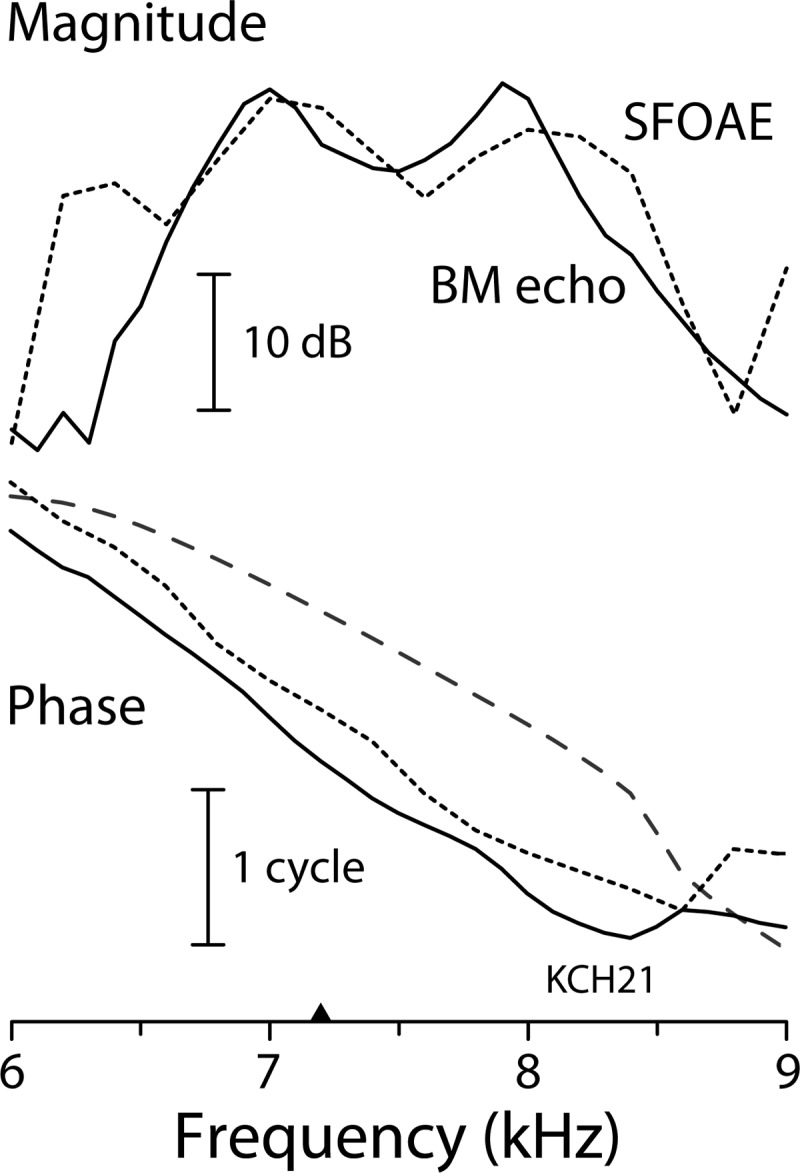
Magnitude and phase of the BM echo spectrum (solid line) and SFOAE spectrum (dotted) obtained from the data of Figs. 5 and 9. The BM echo time waveform was extracted from the BM click response using time windowing [see Fig. 9(C)]. The phase of the main lobe of the BM click response, which serves as the phase reference for the BM echo spectrum, is shown with the dashed line. To aid the comparison, the magnitude spectra have been normalized so that the curves overlap. A triangle along the abscissa marks the approximate CF of the BM measurement location.

F. Wave propagation delays

The SFOAE and BM echo phase-gradient delays computed above provide estimates of roundtrip propagation delays. For SFOAEs, the round-trip delay is from the ear-canal to the region of scattering and back again. For BM echoes, the round-trip delay includes propagation from the measurement point to the region of scattering, reverse travel to the stapes, and then forward travel back to the measurement location. (The measurement location and the region of reflection coincide when both are located near the peak of the traveling wave.) These two delays, both about 1.25 ms for the present data, can be compared with the delay associated with forward travel along the BM. This forward delay can be computed from the phase of the spectrum of the initial burst of the BM click response (dashed line in Fig. 10). Computing the best fit line over the same near-CF interval yields ${\tau }_{\text{BM}}\cong 0.78\pm 0.03\hspace{0.17em}\text{ms}$. Thus the SFOAE and BM echo delays are significantly longer than the forward delay measured on the BM. Computing the delay ratio gives ${\tau }_{\text{SFOAE}}/{\tau }_{\text{BM}}\cong 1.6\pm 0.4$, a value consistent with previous findings from BM and auditory-nerve-fiber measurements in cat, guinea pig, and chinchilla (Shera and Guinan, 2003; Cooper and Shera, 2004; Shera et al., 2008). Since the delays are computed from the phase gradient, they are related to the ripple spacing and corresponding BM and SFOAE phase shifts found in Sec. III C. In particular, the delay ratio closely matches the ratio of SFOAE to BM phase shifts (per ripple period), whose mean value was found to be approximately $1/0.6\hspace{0.17em}\cong 1.67\pm 0.2$ in this animal. As discussed in Sec. III C, the delay ratio is predicted to be less than 2 because of contributions to ${\tau }_{\text{BM}}$ made by the BM impedance (for further details see Shera et al., 2008).

IV. DISCUSSION

Measurements of basilar-membrane motion and stimulus-frequency OAEs made in the same ears demonstrate that the prominent spectral ripples observed in BM mechanical transfer functions at low stimulus intensities (e.g., Rhode, 2007) constitute a mechanical interference pattern analogous to the acoustic interference pattern created in ear-canal pressure by the emission of SFOAEs. When supplemented with mechanical irregularities to scatter forward-traveling waves, active cochlear models reproduce the major features of BM spectral ripples, including their gradual disappearance at higher intensities and their tight correlation with SFOAEs. We conclude that BM spectral ripples arise from multiple internal reflection of waves scattered within the cochlea.

Analysis of the model shows that the magnitude of the BM ripples depends on the product $R{R}_{\text{stapes}}$ [see Eq. (3)], where R is the cochlear reflectance and $R_{\text{stapes}}$ is the stapes reflection coefficient for retrograde waves. According to coherent-reflection theory, R depends both on the distribution of micromechanical irregularities that scatter the wave and on the round-trip gain of the cochlear amplifier. Although all of these quantities can be specified in a cochlear model, none are yet known with any precision experimentally, and all presumably vary from animal to animal.

A. BM ripples and standing waves

According to the model, BM ripples differ significantly from conventional standing-wave interference patterns, which are formed by the superposition of waves traveling in opposite directions (e.g., along a string or within an organ pipe). By contrast, the interference giving rise to BM ripples occurs primarily between two waves traveling in the same (forward) direction. As illustrated heuristically in Fig. 2 and derived from the model in Eq. (3), the two principal waves contributing to the BM interference pattern are (1) the initial forward wave due to the stimulus and (2) the secondary forward wave arising from reflection of the reverse wave at the stapes. (For simplicity, we are ignoring possible higher-order reflections, which generally produce waves of smaller amplitude.) Although a reverse-traveling wave is present in the model, its initial amplitude is typically small in the region of scattering. Since the interference pattern it creates is less prominent, its effect on the motion of the BM can be difficult to detect, especially at frequencies near CF (see Fig. 4, middle panel). However, because the reverse wave is amplified on its way back to the stapes, its relative amplitude grows. After partial reflection at the stapes, the new wave combines with the initial forward wave, effectively adding or subtracting from it depending on the relative phase. The result is a measurable interference pattern near CF. As discussed elsewhere (Sisto et al., 2011; de Boer et al., 2011; Vetesnik and Gummer, 2012), analogous reasoning explains why studies that have used distortion products to look for reverse-traveling waves on the BM have had difficulty finding them (e.g., Ren, 2004; He et al., 2008; de Boer et al., 2008)—the reverse wave, although present, is swamped out by the forward wave that subsequently arises from reflection at the stapes and is then boosted by the cochlear amplifier.

B. Limitations of the model

The computational model we adopted to interpret the experimental results derives from an active transmission-line model of the cochlea supplemented with micromechanical impedance irregularities (e.g., Zweig and Shera, 1995; Talmadge et al., 1998). Although the representation of the cochlear fluids is entirely one-dimensional (i.e., long-wave), extending the hydrodynamics to higher dimensions in order to incorporate the short-wave behavior near the peak of the traveling wave has relatively little effect on the mechanisms of internal reflection relevant here (Shera et al., 2005). Given the compelling agreement we demonstrate between theory and experiment, there appears little to be gained at present by complicating the model further along these lines.

For simplicity, the analytic expressions derived here for P_BM(x) and P_EC include only those terms involving first-order wave scattering within the cochlea (i.e., terms first-order in $\varrho$). Higher-order terms can be obtained using the formulas derived elsewhere (Shera et al., 2005, Sec. IV); all such terms are implicitly included in the “exact” numerical solution and, to the extent the model applies, in the experimental data. Higher-order terms generally involve additional powers of the product $R{R}_{\text{stapes}}$, each additional power representing another roundtrip cycle of internal reflection. Under some circumstances, these higher powers of $R{R}_{\text{stapes}}$ can become significant (e.g., in in vivo or in-silico subjects where the roundtrip gain of the cochlear amplifier is especially large). Indeed, when the product $R{R}_{\text{stapes}}$ approaches 1 in both magnitude and phase, the process of internal reflection can become self-sustaining and continue indefinitely, thereby giving rise to spontaneous otoacoustic emissions and their oscillatory counterparts in BM motion (Shera, 2003; de Boer and Nuttall, 2006).

1. Nonlinear effects

Although the ear-canal and BM rippling patterns appear most pronounced at low sound levels, where the relative amplitudes of reflection-source OAEs are generally largest, the rippling patterns do extend into the compressive regime before gradually disappearing at higher levels. By employing a series of linear models differing in the gain of the cochlear amplifier, we were able to reproduce this behavior qualitatively. Because our models are linear, however, they cannot fully capture certain nonlinear effects, including situations where the effective gain of the cochlear amplifier varies substantially with time. An example is the cochlea's response to transient stimuli, such as clicks, presented at levels that initially push the system strongly into the compressive regime but which then allow the BM response to relax back to quiescence, albeit sometimes via a complex path involving multiple “bursts” of stimulation arising from internal reflection.

Another, more subtle, nonlinear effect involves the influence of multiple internal reflection on the gain of the cochlear amplifier. According to the model, the existence of BM ripples means that BM motion is larger at some frequencies than at others due to constructive and destructive interference between two or more forward-traveling waves. In the compressive regime, however, differences in BM motion (i.e., traveling-wave amplitudes) yield differences in amplifier gain, and these differences in gain in turn affect the traveling-wave amplitudes. In general, the smaller traveling waves propagating at frequencies of ripple valleys experience slightly more gain than do the larger waves propagating at ripple peaks. The net result of these differences in amplifier gain is to reduce the difference between peaks and valleys, thereby decreasing the amplitude of the BM ripples. Although predicted by the conceptual scheme (Fig. 2), this nonlinear effect cannot be captured in a linear model. However, because the BM ripples are generally small (a few dB or less, even in the linear regime), the magnitude of the effect is presumably modest.

C. Prevalence of BM ripples

The correlation between BM ripples and SFOAEs was compelling in all cases where the comparison could be made. We note, however, that not all ears clearly exhibited both phenomena. In particular, whereas measurable SFOAEs could be evoked from 13 of 14 chinchillas in which otoacoustic recordings were attempted, only nine of these ears exhibited measurable BM ripples. The reasons for this difference in prevalence remain unclear, although issues such as the frequency resolution and signal-to-noise ratio of the data presumably play some role. Table II in the Appendix provides details of the animal preparation and recording conditions (e.g., gender, weight, and age; CAP thresholds; bead composition and radial locations on the BM; cochlear amplifier gains; SFOAE levels; BM ripple magnitudes; etc.). Other than obvious relationships anticipated from previous work (e.g., cochlear amplifier gain and SFOAE level vary inversely with CAP threshold), our examination of these records reveals no compelling correlations that might help account for interanimal variations in the magnitude of BM ripples, including their apparent absence in some preparations. Although the model indicates that the amplitudes of the BM and ear-canal interference ripples can vary independently (e.g., the BM ripples are much more sensitive to the value of $R_{\text{stapes}}$, which presumably varies between animals), more data are needed to address this issue further.

TABLE II.

Summary of the experiments. Entries and methodological details are explained in the text.

Animal	Date	Duration (hh:mm)	Mass (g)	Gender	Age (mos.)	CAP before surgery (dB SPL)	CAP during BM (dB SPL)	CAP loss (dB)	Probe level for SFOAEs (dB SPL)	SFOAE re probe before surgery (dB)	SFOAE re probe during BM (dB)	SFOAE change (dB)	Cover	Type of beads
KCH08	07 Oct 04	15:15	408	M	—	18.5	19	0.5	40	−31.7	−34.1	−2.4	wire + glass	polystyrene
KCH12	18 Oct 07	12:30	286	M	<12	21	27	6	40	−21.3	−23.7	−2.4	glass	polystyrene
KCH13	29 Nov 07	12:00	694	F	>24	25	25	0	40	−18.5	−18.0	+0.5	wire	polystyrene
KCH21	08 Jan 09	09:00	483	M	<8	12.5	14	1.5	20,30	−12.2	−13.9	−1.7	wire	hollow
KCH22	16 Jan 09	08:21	480	M	<8	19.5	28	8.5	20	−27.1	−29.8	−2.7	wire + glass	hollow
KCH24	26 Jan 09	14:20	468	F	<6	6.5	15	8.5	20	−10.7	−13.6	−2.9	wire + glass	hollow
KCH25	15 Mar 10	04:52	280	M	—	17	21	4	30	−33.0	N/A	N/A	wire	hollow
KCH26	19 Apr 10	08:25	610	F	>36	22	23	1	30	−29.3	−30.5	−1.2	wire + glass	hollow
KCH29	3 Sep 10	09:05	487	F?	<12	21.5	27	5.5	30	−33.7	−35.7	−2.0	glass	hollow
KCH30	6 Sep 10	07:18	460	M	<12	13	40.5	27.5	30	−18.7	N/A	N/A	wire	hollow
KCH31	13 Oct 10	09:43	430	M	4.5	23	26	3	30	−23.3	−24.3	−1.0	glass	hollow
KCH32	14 Oct 10	09:15	587	M	4.5	19.5	23	3.5	30	−25.6	−27.4	−1.8	glass	hollow
KCH33	22 Jun 11	09:30	400	F	4	13.5	14.5	1	30	−24.0	−16.9	+7.1	wire + glass	stainless
KCH34	24 Jun 11	08:50	700	F	>24	11.5	15	3.5	30	−24.5	−29.5	−5.0	glass	hollow

Animal	# of beads	Meas ID	Position on BM	CF (kHz)	Max BM gain re ME (dB)	NL/CA (dB)	Compression threshold (dB SPL)	Wax/wane (# lobes)	Ripple (dB)
KCH08	multi	bead 1,4	N/A	8.0	54	52	15	1	2.6
KCH12	multi (>10)	bm 2–4	middle	7.2	61	34	28	1	1.7
KCH13	multi (>3)	bead 2–10	N/A	5.9	69	35	29	1–2?	—
KCH21	multi	bead 1,2	OPC feet	7.1	73	50	15	3–5	2.6
KCH22	2	bead 1	50% across	7.0	54	>25	30	1	1.4
		bead 2	50% (100 μm apical)	7.2	63	>34	30	1	2.5
KCH24	multi (>3, 3 times)	bead 3,4	arcuate zone	9.2	66	48	14	1	1.9
		bead 5	middle + apical	8.7	68	45	15	1–2?	1.3
		bead 6	pectinate + basalmost	9.1	77	56	17	1–2?	2.0
KCH25	2	bm 1	50% across	6.9	71	>34	23	1–2	—
		bm 2	75% (pectinate)	7.0	48	>19	35	1–2?	—
KCH26	1	bm 2,3	N/A	5.9	64	42	30	1	—
KCH29	2	bm 3	middle	8.0	69	48	20	1	—
KCH30	2	bead 1,2	N/A	8.0	—	17	50	1	—
KCH31	>3	bead 5	middle	8.6	86	60	10	2	1.7
KCH32	1	bm 1–4	middle	6.9	71	>52	20	1–3	2.2
KCH33	multi (>3, 3 times)	bm 1,2	outer edge	7.5	55	>52	12	2?	2.9
		bm 3	middle	8.0	82	>34	20	5	5.8
		bm 4,5	middle (200 μm apical)	6.3	70	>45	22	2?	6.8
KCH34	1	bm 1–5	OPC feet	6.9	76	60	8	2	2.6

D. Origin of fine structure in BM and ANF click responses

Both the model and the measurements reported here demonstrate that BM spectral ripples can manifest themselves in the time domain as multiple or prolonged lobes in the BM click response (Shera, 2001a). Our results thus demonstrate that these common features of BM and auditory-nerve-fiber (ANF) click responses can result from the multiple internal reflection of otoacoustic energy. Previous explanations for waxing and waning in the click-response envelope—such as beating between multiple vibrational modes in the organ of Corti (Lin and Guinan, 2000, 2004) or interactions among coupled nonlinear oscillators (Zweig, 2003; Aranyosi, 2006)—all involve hypothetical processes local to the measurement location. We have shown, however, that response features that appear to involve complex local interactions can arise via global mechanisms involving multiple reflection and wave propagation in the cochlea. Similar global processes can account for spontaneous OAEs (Shera, 2003; de Boer and Nuttall, 2006). Although our results do not rule out other explanations for the fine structure often seen in BM and ANF click responses, they do suggest that mechanisms involving previously well known phenomena (i.e., otoacoustic emissions) can account for at least some subset of the data. The click response features least likely to be accounted for by multiple internal reflection are patterns of waxing and waning that persist, or even grow, at high sound levels. Although modulations in the gain of the cochlear amplifier during the time course of the response complicate any easy interpretation, the relative contribution of otoacoustic mechanisms is likely to be the smallest at high intensities.

E. Possible experimental tests

Unable to properly pursue them ourselves, we offer a few anecdotal observations with the hope of inspiring others to perform additional experimental tests of the model. Although the generation of SFOAEs (and, presumably, BM ripples) occurs naturally by scattering from intrinsic mechanical irregularities, the model suggests trying to modify the emissions by introducing artificial perturbations. We attempted to do this in one of the present experiments (KCH33) by using relatively large (25–40 μm diameter) stainless-steel beads instead of our standard, much lighter beads. Whereas the standard beads have a specific gravity (s.g.) close to that of the surrounding water, the stainless steel beads have specific gravity eight times larger and, we reasoned, might therefore affect the motion of the BM.⁹ Interestingly, in this one experiment (Fig. 6) the SFOAE levels increased substantially after opening the cochlea and dropping the beads on the BM (usually emission levels decrease slightly, presumably because of trauma). Thus, by mass loading the BM, the beads may have augmented the impedance irregularities and enhanced the subsequent wave scattering (cf. Sellick et al., 1983).

Perhaps the most interesting prediction of the model is that the pattern of BM ripples depends not only on mechanisms within the cochlea (i.e., on wave scattering) but also on the stapes reflection coefficient, $R_{\text{stapes}}$, whose value at any given frequency quantifies the load placed on the cochlea by the middle ear and outside world. Direct experimental manipulation of this load (e.g., by reversibly modifying the middle ear) provides an opportunity to test this prediction. In one experiment (KCH08) we placed, and later removed, a small piece of wire (2.2 mg) on the shaft of the manubrium near the umbo. Although the mass load did reversibly modify middle-ear and BM responses at low frequencies, especially near a notch in the motion of the incus at 3 kHz, it had no obvious reversible effect at frequencies closer to CF (∼8 kHz) or on the pattern of waxing and waning seen in the click response. Although the mass load evidently altered the mode of middle-ear vibration at low frequencies, its influence appeared negligible on the BM in the frequency range of interest. Even if the load had modified the near-CF rippling pattern, quantitative interpretation would have remained challenging, since we lacked independent means to determine how (or whether) the load changed the value of $R_{\text{stapes}}$.

F. The mode of reverse OAE propagation

Both the histogram in Fig. 8—which finds approximately 0.5 cycles of BM phase shift per ripple period (i.e., for every cycle of SFOAE phase)—and the comparison of near-CF BM and SFOAE phase gradients in Sec. III E indicate that by the time they reach the ear canal, SFOAEs have acquired substantially greater phase shifts than can be accounted for by the forward-traveling wave on the BM (by a factor of roughly 1.6–1.7 in these data). Because middle-ear delay appears negligible compared to cochlear delay in chinchilla (Ruggero et al., 1990; Songer and Rosowski, 2007), most of this additional phase shift (delay) must arise within the cochlea. According to the coherent-reflection model, the additional OAE delay arises from back-propagation of transverse, pressure-difference waves along the cochlear partition. Because pressure-difference waves couple to the motion of the basilar membrane, their wave speeds are determined, in part, by the mechanics of the partition and are substantially slower than the speed of sound in the fluid. (For this reason, they are known as “slow waves.”) The result of this slow-wave propagation is that OAEs are significantly delayed on their way back to the stapes and ear canal. The alternative, “fast-wave” model of OAE propagation posits that otoacoustic energy travels within the cochlea via longitudinal, compressional waves that travel at the speed of sound in the fluid (e.g., Wilson, 1980; Ren, 2004). This speed is so high (∼1500 m/s), and the distances involved are so short (∼3.5 mm for the 8 kHz place in chinchilla), that the propagation delays are negligible (∼2.4 μs). Since estimated fast-wave delays are some 200 times smaller than required to account for the difference between the measured SFOAE and BM phase gradients, our data indicate that otoacoustic delays are much too long to be explained by the fast-wave model of OAE propagation. Although fast-wave modes provide an alternate means for otoacoustic energy to escape from the cochlea, they are evidently not the dominant mode of propagation for mammalian stimulus-frequency OAEs.

G. Comparison with BM ripples at high sound levels

Our subject here has been the rippling patterns observed in measurements of BM motion at sound levels near the threshold of hearing. In addition to these low-level patterns, however, ripples are often seen at much higher sound levels. Indeed, in the paper reporting the data reproduced in Fig. 1, Rhode (2007) passed over the low-level ripples to focus on the ripples and notches evident at high stimulus levels, which can be seen in the lower right-hand corner of both the amplitude and phase panels in Fig. 1. Unlike the low-level ripples, which appear most prominent for frequencies at and below CF, high-level ripples are seen predominantly above CF, where they are thought to result from interference between BM responses to slow and fast pressure waves (Cooper and Rhode, 1996; Olson, 1999; Rhode, 2007). Both the low- and high-level BM ripples thus occur when an additional drive interferes with the motion produced by the primary (slow) traveling wave. In each case, the ripple spacing is determined by the rate of relative phase rotation between the two drives at the measurement location. Figure 11 demonstrates that these rates are very different for the two sets of ripples. At low sound levels, the data of Rhode (2007) are consistent with the results shown in Figs. 7 and 8, which indicate that the low-level BM ripples are spaced at intervals corresponding to approximately one-half cycle of BM phase (dotted lines with leftward arrows in Fig. 11). As explained in Sec. III C, the half-cycle shift arising from forward wave travel is matched by a half-cycle shift from reverse wave travel, so that the total phase shift between ripple peaks amounts to one cycle, as required. The ripple spacing thus agrees with theoretical predictions based on multiple internal reflection involving round-trip slow-wave propagation. At high sound levels, by contrast, the ripples are spaced at wider intervals, corresponding to one full cycle of BM phase (dotted lines with rightward arrows in Fig. 11). As pointed out by Rhode (2007) and others, the full cycle of BM phase rotation between ripple peaks (or notches) is consistent with interference from the fast pressure wave, whose speed is very high and whose phase is therefore nearly constant compared to that of the BM traveling wave (Olson, 1999). In this case, therefore, the entirety of the required phase shift arises from the forward-traveling slow wave.

FIG. 11.

High- and low-level ripple spacing and BM phase. The figure shows magnitudes (top) and phases (bottom) of BM mechanical transfer functions (Rhode, 2007). Responses are shown at the four lowest sound levels (solid black lines, for 5, 10, 15, 20 dB SPL) and the three highest sound levels (dashed gray lines, for 85, 90, 95 dB SPL) measured. The same magnitude data, including data at intermediate levels, are shown in Fig. 1. As in Fig. 7, the dotted black lines with leftward pointing arrows locate values of BM phase corresponding to approximate low-level ripple peaks. On average, the low-level BM ripples are spaced at intervals corresponding to about one-half cycle of BM phase. The dotted gray lines with rightward pointing arrows locate values of BM phase corresponding to approximate high-level notches. The high-level ripples are spaced at intervals corresponding to about one full cycle of BM phase. Adapted from Figs. 2 and 4 of Rhode (2007).

Why are the two different types of BM ripples seen at opposite ends of the intensity range and, for the most part, on opposite sides of CF? In both cases, prominent ripples only appear when the two interfering drives have similar amplitudes at the measurement location. High sound levels and frequencies above CF provide the right conditions for interference from fast waves. Although generally dwarfed by the slow-wave (or transpartition) pressure, the fast-wave pressure can provide a significant drive when the gain provided to the slow wave remains small and/or its attenuation becomes large. These conditions occur together at high sound levels, where hair-cell based slow-wave amplification has little effect, and at frequencies in the cutoff region above CF, where the amplitude of the slow wave falls dramatically (Olson, 1999). Conversely, frequencies below CF and low sound levels favor interference due to the multiple internal reflection of slow waves. Slow-wave propagation occurs only at frequencies near or below CF, and producing a secondary forward-traveling wave similar in amplitude to the primary wave (i.e., within 10–20 dB) requires strong scattering (i.e., large impedance irregularities) and/or considerable amplification of the reverse-traveling wave. Both conditions are most likely to occur at low sound levels, where cochlear amplification of slow waves is strongest and where micromechanical irregularities dominated by cell-to-cell variations in the strength of the active forces would presumably be largest. Although difficulties locating reverse-traveling slow waves directly on the basilar membrane (e.g., Ren, 2004; Ren et al., 2006; He et al., 2008) have fostered doubts about whether reverse slow waves really do (or can) exist, their evident role in producing low-level interference patterns observable in both BM motion [e.g., by both Rhode (2007) and ourselves] and in ear-canal pressure (i.e., OAEs) provides a compelling existence proof.

APPENDIX: METHODOLOGICAL AND EXPERIMENTAL DETAILS

Table II provides a capsule summary of the experiments and briefly summarizes important methodological details. Many entries are self-explanatory; the others are described in the following paragraphs.

Duration: gives the time interval between the initial dose of anesthesia and the time of death (i.e., the duration of the in vivo part of the experiment).

CAP thresholds: gives the compound action potential (CAP) thresholds at CF. Thresholds were assessed using an automated tracking procedure (Taylor and Creelman, 1967) that determines the SPL necessary to evoke a constant amplitude response from a silver wire electrode placed near the niche of the round window. Our typical threshold criterion was 10 μV peak-to-peak (N₁–P₁). CAP threshold audiograms (Johnstone et al., 1979) were assessed from 1–15 kHz (in 500 Hz steps) both before and after opening the cochlea and making BM and SFOAE measurements. Changes in tone-evoked CAP thresholds are excellent indicators of the cochlea's localized (i.e., CF-specific) physiology (Sellick et al., 1982).

SFOAE levels: gives the mean near-CF emission level expressed relative to the probe level, L_p, which varied from 20 to 40 dB SPL (30 dB SPL in most experiments). Levels are averaged over the frequency range of 5–8 kHz. SFOAEs were derived using an ear-canal pressure suppression technique similar to that described by Shera and Guinan (1999). SFOAEs were measured both before and after opening the cochlea and making the BM measurements. Changes in the SFOAE levels are expected to reflect localized changes in cochlear mechanics.

Cover: gives the method used to control the perilymphatic meniscus above the opening into the scala tympani. Our standard approach was to cover the scala tympani hole with a small fragment of a glass cover slip (“glass”), but in many instances this had an undesirable outcome (because the glass often refracted the incident light the wrong way, so that we lost our image of the BM). Our usual solution to this problem was to prop or “wedge” the cover glass up to provide a more favorable angle of incidence—this was done using a short piece of metal wire placed immediately adjacent to the hole above the BM (giving the “wire + glass” condition). However, in a few cases this approach brought further problems (e.g., the fluid-filled tunnel beneath glass and wire could act as a capillary that sucked nearby blood and debris into the scala tympani). In such cases, we resorted to a wire-alone solution, in which the short piece of wire was used purely to shape the perilymphatic meniscus and “bend” the image of the BM. In the wire alone condition, we rely on the fact that the BM/incus gain is high in order to limit the effects of sound-induced perilymphatic movements.

Type of bead: gives the composition of the beads used to enhance reflection of the incident laser light from the BM. “Polystyrene” ≡ 20 μm-diameter spherical polystyrene microbeads (Polysciences, Inc.; s.g. 1.05 g/cm) that had been sputter-coated with gold (to a depth of around 20 nm). “Hollow” ≡ 20–25 μm-diameter silver-coated hollow glass microbeads (Micro Sphere Technology, UK; s.g. 1.05–1.2 g/cm). “Stainless” ≡ 24–40 μm-diameter stainless-steel beads (Duke Scientific, s.g. ∼8 g/cm).

# beads: gives the number of beads placed on the BM at any given time. In some experiments, multiple recording sessions were used, each with a different number and distribution of beads. In such cases, the beads from the earlier recording sessions were either “wicked” or washed away from the BM with perilymph, or, in the case of the stainless steel beads, removed from the cochlea entirely using a magnetic probe.

Measurement ID: gives the mnemonic used to refer to a set of recordings from an individual bead. Each bead may be recorded multiple times, and therefore have multiple IDs; different beads always have different IDs.

Position on the BM: gives the approximate position of the recording location across the width of the BM. OPC ≡ outer pillar cell, positioned approximately one-third of the way across the BM from the inner spiral lamina.

CF: gives the characteristic frequency of the recording site. The CF was determined from the BM/middle-ear transfer functions at the lowest SPL recorded.

Max BM gain: gives the maximum gain of the BM vibrations, relative to the incus and/or stapes vibrations, at the CF of the BM recording site. This was determined from the BM/middle-ear (ME) transfer functions at the lowest SPL presented.

NL/CA: gives a lower bound on the amount of compressive nonlinearity [or “cochlear amplifier (CA) gain”] observed at the CF of each recording site. The values were determined by comparing the BM's sensitivity at low SPLs, where the CF responses grow nearly linearly (i.e., at roughly 1 dB/dB), and at high SPLs, where the responses can grow much more slowly (e.g., at 0.1 dB/dB). In all cases the input-output behavior at CF remained compressive to the highest SPLs tested (typically 85–90 dB SPL); therefore, the values in the table must be considered lower bounds. Greater than symbols (>) are used to point out a few cases where the maximum SPLs tested were substantially lower than 85–90 dB SPL, so that the actual amount of nonlinearity is likely to have been underestimated substantially.

Compression threshold: gives the sound level at which the magnitude of the BM/ME transfer function at CF decreased by 1 dB from its maximum at low sound levels (“−1 dB threshold”). The value was determined by interpolation from the input-output function at CF.

Wax/wane: gives the number of lobes in the BM's click responses as determined by visual inspection. Question marks (?) denote instances where the separation of one lobe from another was incomplete, but still obvious visually.

Ripple: gives the size of the near-CF ripples in the BM/ME transfer functions, judged as maximum peak-to-peak deviations from a smooth curve (10th-order polynomial) fit to the magnitude of the BM/ME transfer function tip. More precisely, the ripple magnitudes in dB are defined as $20\hspace{0.17em}{\text{log}}_{10}[(1+\alpha )/(1-\alpha )]$, where $\alpha \equiv A/2S$, S represents the value of the smooth curve, and A is the peak-to-peak variation of the residual.

REFERENCES

- 1.Aranyosi, A. J. (2006). “ A ‘twin-engine’ model of level-dependent cochlear motion,” in Auditory Mechanisms: Processes and Models, edited by Nuttall A. L., Ren T., Gillespie P., Grosh K., and de Boer E. (World Scientific, Singapore: ), pp. 500–501 [Google Scholar]
- 2.Cooper, N. P. (1999). “ An improved heterodyne laser interferometer for use in studies of cochlear mechanics,” J. Neurosci. Meth. 88, 93–102 10.1016/S0165-0270(99)00017-5 [DOI] [PubMed] [Google Scholar]
- 3.Cooper, N. P. , and Rhode, W. S. (1992). “ Basilar membrane mechanics in the hook region of cat and guinea-pig cochleae: Sharp tuning and nonlinearity in the absence of baseline position shifts,” Hear. Res. 63, 163–190 10.1016/0378-5955(92)90083-Y [DOI] [PubMed] [Google Scholar]
- 4.Cooper, N. P. , and Rhode, W. S. (1996). “ Fast travelling waves, slow travelling waves and their interactions in experimental studies of apical cochlear mechanics,” Aud. Neurosci. 2, 207–217 [Google Scholar]
- 5.Cooper, N. P. , and Shera, C. A. (2004). “ Backward traveling waves in the cochlea? Comparing basilar-membrane vibrations and otoacoustic emissions from individual guinea-pig ears,” Assoc. Res. Otolaryngol. Abs. 27, 1008 [Google Scholar]
- 6.de Boer, E., and Nuttall, A. L. (2006). “ Spontaneous basilar-membrane oscillation (SBMO) and coherent reflection,” J. Assoc. Res. Otolaryngol. 7, 26–37 10.1007/s10162-005-0020-9 [DOI] [PMC free article] [PubMed] [Google Scholar]
- 7.de Boer, E., Shera, C. A. , and Nuttall, A. L. (2011). “ Tracing distortion product (DP) waves in a cochlear model,” in What Fire is in Mine Ears: Progress in Auditory Biomechanics, edited by Shera C. A. and Olson E. S. (AIP, Melville, NY: ), 557–562 [DOI] [PMC free article] [PubMed] [Google Scholar]
- 8.de Boer, E., Zheng, J., Porsov, E., and Nuttall, A. L. (2008). “ Inverted direction of wave propagation (IDWP) in the cochlea,” J. Acoust. Soc. Am. 123, 1513–1521 10.1121/1.2828064 [DOI] [PMC free article] [PubMed] [Google Scholar]
- 9.Elliot, E. (1958). “ A ripple effect in the audiogram,” Nature 181, 1076. 10.1038/1811076a0 [DOI] [PubMed] [Google Scholar]
- 10.Guinan, J. J. , and Cooper, N. P. (2008). “ Medial olivocochlear efferent inhibition of basilar-membrane responses to clicks: Evidence for two modes of cochlear mechanical excitation,” J. Acoust. Soc. Am. 124, 1080–1092 10.1121/1.2949435 [DOI] [PMC free article] [PubMed] [Google Scholar]
- 11.He, W., Fridberger, A., Porsov, E., Grosh, K., and Ren, T. (2008). “ Reverse wave propagation in the cochlea,” Proc. Natl. Acad. Sci. USA 105, 2729–2733 10.1073/pnas.0708103105 [DOI] [PMC free article] [PubMed] [Google Scholar]
- 12.Johnstone, J. R. , Alder, V. A. , Johnstone, B. M. , Roberston, D., and Yates, G. K. (1979). “ Cochlear action potential threshold and single unit thresholds,” J. Acoust. Soc. Am. 65, 247–254 10.1121/1.382244 [DOI] [PubMed] [Google Scholar]
- 13.Kalluri, R., and Shera, C. A. (2001). “ Distortion-product source unmixing: A test of the two-mechanism model for DPOAE generation,” J. Acoust. Soc. Am. 109, 622–637 10.1121/1.1334597 [DOI] [PubMed] [Google Scholar]
- 14.Kalluri, R., and Shera, C. A. (2007). “ Comparing stimulus-frequency otoacoustic emissions measured by compression, suppression, and spectral smoothing,” J. Acoust. Soc. Am. 122, 3562–3575 10.1121/1.2793604 [DOI] [PubMed] [Google Scholar]
- 15.Kemp, D. T. (2002). “ Exploring cochlear status with otoacoustic emissions: The potential for new clinical applications,” in Otoacoustic Emissions: Clinical Applications, 2nd ed., edited by Robinette M. S. and Glattke T. J. (Thieme, New York: ), pp. 1–47 [Google Scholar]
- 16.Kemp, D. T. , and Chum, R. A. (1980). “ Observations on the generator mechanism of stimulus frequency acoustic emissions — Two tone suppression,” in Psychophysical Physiological and Behavioural Studies in Hearing, edited by Brink G. V. D. and Bilsen F. A. (Delft University Press, Delft: ), pp. 34–42 [Google Scholar]
- 17.Lin, T., and Guinan, J. J. (2000). “ Auditory-nerve-fiber responses to high-level clicks: Interference patterns indicate that excitation is due to the combination of multiple drives,” J. Acoust. Soc. Am. 107, 2615–2630 10.1121/1.428648 [DOI] [PubMed] [Google Scholar]
- 18.Lin, T., and Guinan, J. J. (2004). “ Time-frequency analysis of auditory-nerve-fiber and basilar-membrane click responses reveal glide irregularities and non-characteristic-frequency skirts,” J. Acoust. Soc. Am. 116, 405–416 10.1121/1.1753294 [DOI] [PubMed] [Google Scholar]
- 19.Long, G. R. (1984). “ The microstructure of quiet and masked thresholds,” Hear. Res. 15, 73–87 10.1016/0378-5955(84)90227-2 [DOI] [PubMed] [Google Scholar]
- 20.Olson, E. S. (1999). “ Direct measurement of intra-cochlear pressure waves,” Nature 402, 526–529 10.1038/990092 [DOI] [PubMed] [Google Scholar]
- 21.Ravicz, M. E. , and Rosowski, J. J. (2012). “ A new estimate of the middle-ear transmission matrix in chinchilla,” Assoc. Res. Otolaryngol. Abs. 35, 126 [Google Scholar]
- 22.Ravicz, M. E. , Slama, M. C. C. , and Rosowski, J. J. (2010). “ Middle-ear pressure gain and cochlear partition differential pressure in chinchilla,” Hear. Res. 263, 16–25 10.1016/j.heares.2009.11.014 [DOI] [PMC free article] [PubMed] [Google Scholar]
- 23.Recio, A., Rich, N. C. , Narayan, S. S. , and Ruggero, M. A. (1998). “ Basilar-membrane responses to clicks at the base of the chinchilla cochlea,” J. Acoust. Soc. Am. 103, 1972–1989 10.1121/1.421377 [DOI] [PMC free article] [PubMed] [Google Scholar]
- 24.Ren, T. (2004). “ Reverse propagation of sound in the gerbil cochlea,” Nat. Neurosci. 7, 333–334 10.1038/nn1216 [DOI] [PubMed] [Google Scholar]
- 25.Ren, T., He, W., Scott, M., and Nuttall, A. L. (2006). “ Group delay of acoustic emissions in the ear,” J. Neurophysiol. 96, 2785–2791 10.1152/jn.00374.2006 [DOI] [PubMed] [Google Scholar]
- 26.Rhode, W. S. (2007). “ Basilar membrane mechanics in the 6–9 kHz region of sensitive chinchilla cochleae,” J. Acoust. Soc. Am. 121, 2792–2804 10.1121/1.2718397 [DOI] [PubMed] [Google Scholar]
- 27.Ruggero, M. A. , Rich, N. C. , Robles, L., and Shivapuja, B. G. (1990). “ Middle-ear response in the chinchilla and its relationship to mechanics at the base of the cochlea,” J. Acoust. Soc. Am. 87, 1612–1629 10.1121/1.399409 [DOI] [PMC free article] [PubMed] [Google Scholar]
- 28.Ruggero, M. A. , Robles, L., and Rich, N. C. (1986). “ Basilar membrane mechanics at the base of the chinchilla cochlea. II. Responses to low-frequency tones and relationship to microphonics and spike initiation in the VIII nerve,” J. Acoust. Soc. Am. 80, 1375–1383 10.1121/1.394390 [DOI] [PubMed] [Google Scholar]
- 29.Sellick, P. M. , Patuzzi, R., and Johnstone, B. M. (1982). “ Measurement of basilar membrane motion in the guinea pig using the Mössbauer technique,” J. Acoust. Soc. Am. 72, 131–141 10.1121/1.387996 [DOI] [PubMed] [Google Scholar]
- 30.Sellick, P. M. , Yates, G. K. , and Patuzzi, R. (1983). “ The influence of Mössbauer source size and position on phase and amplitude measurements of the guinea pig basilar membrane,” Hear. Res. 10, 101–108 10.1016/0378-5955(83)90020-5 [DOI] [PubMed] [Google Scholar]
- 31.Shera, C. A. (2001a). “ The effect of reflection emissions on impulse responses of the basilar membrane and the auditory nerve,” Assoc. Res. Otolaryngol. Abs. 24, 815 [Google Scholar]
- 32.Shera, C. A. (2001b). “ Intensity-invariance of fine time structure in basilar-membrane click responses: Implications for cochlear mechanics,” J. Acoust. Soc. Am. 110, 332–348 10.1121/1.1378349 [DOI] [PubMed] [Google Scholar]
- 33.Shera, C. A. (2003). “ Mammalian spontaneous otoacoustic emissions are amplitude-stabilized cochlear standing waves,” J. Acoust. Soc. Am. 114, 244–262 10.1121/1.1575750 [DOI] [PubMed] [Google Scholar]
- 34.Shera, C. A. , and Cooper, N. P. (2009). “ Wave-interference patterns on the basilar membrane: Testing models of OAE propagation,” Assoc. Res. Otolaryngol. Abs. 32, 56 [Google Scholar]
- 35.Shera, C. A. , and Guinan, J. J. (1999). “ Evoked otoacoustic emissions arise by two fundamentally different mechanisms: A taxonomy for mammalian OAEs,” J. Acoust. Soc. Am. 105, 782–798 10.1121/1.426948 [DOI] [PubMed] [Google Scholar]
- 36.Shera, C. A. , and Guinan, J. J. (2003). “ Stimulus-frequency-emission group delay: A test of coherent reflection filtering and a window on cochlear tuning,” J. Acoust. Soc. Am. 113, 2762–2772 10.1121/1.1557211 [DOI] [PubMed] [Google Scholar]
- 37.Shera, C. A. , Tubis, A., and Talmadge, C. L. (2005). “ Coherent reflection in a two-dimensional cochlea: Short-wave versus long-wave scattering in the generation of reflection-source otoacoustic emissions,” J. Acoust. Soc. Am. 118, 287–313 10.1121/1.1895025 [DOI] [PubMed] [Google Scholar]
- 38.Shera, C. A. , Tubis, A., and Talmadge, C. L. (2008). “ Testing coherent reflection in chinchilla: Auditory-nerve responses predict stimulus-frequency emissions,” J. Acoust. Soc. Am. 124, 381–395 10.1121/1.2917805 [DOI] [PMC free article] [PubMed] [Google Scholar]
- 39.Shera, C. A. , and Zweig, G. (1991). “ Reflection of retrograde waves within the cochlea and at the stapes,” J. Acoust. Soc. Am. 89, 1290–1305 10.1121/1.400654 [DOI] [PubMed] [Google Scholar]
- 40.Shera, C. A. , and Zweig, G. (1992). “ Analyzing reverse middle-ear transmission: Noninvasive Gedankenexperiments,” J. Acoust. Soc. Am. 92, 1371–1381 10.1121/1.403930 [DOI] [PubMed] [Google Scholar]
- 41.Shera, C. A. , and Zweig, G. (1993). “ Noninvasive measurement of the cochlear traveling-wave ratio,” J. Acoust. Soc. Am. 93, 3333–3352 10.1121/1.405717 [DOI] [PubMed] [Google Scholar]
- 42.Sisto, R., Moleti, A., Botti, T., Bertaccini, D., and Shera, C. A. (2011). “ Distortion products and backward traveling waves in nonlinear active models of the cochlea,” J. Acoust. Soc. Am. 129, 3141–3152 10.1121/1.3569700 [DOI] [PMC free article] [PubMed] [Google Scholar]
- 43.Songer, J. E. , and Rosowski, J. J. (2007). “ Transmission matrix analysis of the chinchilla middle ear,” J. Acoust. Soc. Am. 122, 932–942 10.1121/1.2747157 [DOI] [PMC free article] [PubMed] [Google Scholar]
- 44.Talmadge, C. L. , Tubis, A., Long, G. R. , and Piskorski, P. (1998). “ Modeling otoacoustic emission and hearing threshold fine structures,” J. Acoust. Soc. Am. 104, 1517–1543 10.1121/1.424364 [DOI] [PubMed] [Google Scholar]
- 45.Taylor, M. M. , and Creelman, C. D. (1967). “ PEST: Efficient estimates on probability functions,” J. Acoust. Soc. Am. 41, 782–787 10.1121/1.1910407 [DOI] [Google Scholar]
- 46.Thomas, I. B. (1975). “ Microstructure of the pure-tone threshold,” J. Acoust. Soc. Am. 57, Suppl. 1 , S26–S27 10.1121/1.1995148 [DOI] [Google Scholar]
- 47.Vetesnik, A., and Gummer, A. W. (2012). “ Transmission of cochlear distortion products as slow waves: A comparison of experimental and model data,” J. Acoust. Soc. Am. 131, 3914–3934 10.1121/1.3699207 [DOI] [PubMed] [Google Scholar]
- 48.Wilson, J. P. (1980). “ Model for cochlear echoes and tinnitus based on an observed electrical correlate,” Hear. Res. 2, 527–532 10.1016/0378-5955(80)90090-8 [DOI] [PubMed] [Google Scholar]
- 49.Zweig, G. (1991). “ Finding the impedance of the organ of Corti,” J. Acoust. Soc. Am. 89, 1229–1254 10.1121/1.400653 [DOI] [PubMed] [Google Scholar]
- 50.Zweig, G. (2003). “ Cellular cooperation in cochlear mechanics,” in Biophysics of the Cochlea: From Molecules to Models, edited by Gummer A. W. (World Scientific, Singapore: ), pp. 315–330 [Google Scholar]
- 51.Zweig, G., and Shera, C. A. (1995). “ The origin of periodicity in the spectrum of evoked otoacoustic emissions,” J. Acoust. Soc. Am. 98, 2018–2047 10.1121/1.413320 [DOI] [PubMed] [Google Scholar]
- 52.Zwicker, E., and Schloth, E. (1984). “ Interrelation of different oto-acoustic emissions,” J. Acoust. Soc. Am. 75, 1148–1154 10.1121/1.390763 [DOI] [PubMed] [Google Scholar]