Liver segmentation in contrast enhanced CT data using graph cuts and interactive 3D segmentation refinement methods

Abstract

Purpose:

Liver segmentation is an important prerequisite for the assessment of liver cancer treatment options like tumor resection, image-guided radiation therapy (IGRT), radiofrequency ablation, etc. The purpose of this work was to evaluate a new approach for liver segmentation.

Methods:

A graph cuts segmentation method was combined with a three-dimensional virtual reality based segmentation refinement approach. The developed interactive segmentation system allowed the user to manipulate volume chunks and/or surfaces instead of 2D contours in cross-sectional images (i.e, slice-by-slice). The method was evaluated on twenty routinely acquired portal-phase contrast enhanced multislice computed tomography (CT) data sets. An independent reference was generated by utilizing a currently clinically utilized slice-by-slice segmentation method. After 1 h of introduction to the developed segmentation system, three experts were asked to segment all twenty data sets with the proposed method.

Results:

Compared to the independent standard, the relative volumetric segmentation overlap error averaged over all three experts and all twenty data sets was 3.74%. Liver segmentation required on average 16 min of user interaction per case. The calculated relative volumetric overlap errors were not found to be significantly different [analysis of variance (ANOVA) test,p = 0.82] between experts who utilized the proposed 3D system. In contrast, the time required by each expert for segmentation was found to be significantly different (ANOVA test, p = 0.0009). Major differences between generated segmentations and independent references were observed in areas were vessels enter or leave the liver and no accepted criteria for defining liver boundaries exist. In comparison, slice-by-slice based generation of the independent standard utilizing a live wire tool took 70.1 min on average. A standard 2D segmentation refinement approach applied to all twenty data sets required on average 38.2 min of user interaction and resulted in statistically not significantly different segmentation error indices (ANOVA test, significance level of 0.05).

Conclusions:

All three experts were able to produce liver segmentations with low error rates. User interaction time savings of up to 71% compared to a 2D refinement approach demonstrate the utility and potential of our approach. The system offers a range of different tools to manipulate segmentation results, and some users might benefit from a longer learning phase to develop efficient segmentation refinement strategies. The presented approach represents a generally applicable segmentation approach that can be applied to many medical image segmentation problems.

I. INTRODUCTION

Liver cancer is a major health problem. The World Health Organization (WHO) estimates that liver cancer accounts for more than 600 000 deaths per year.¹ A careful evaluation of each patient is required to select one or a combination of the many different treatment options available, which include surgical resection, chemotherapy, cryosurgery, radiofrequency ablation, liver transplantation, etc. Tomographic imaging modalities like x-ray computed tomography (CT) play an important role in this selection process. For example, in the case of hepatocellular carcinoma (HCC), liver resection has evolved as the treatment of choice, but not all patients are suitable for resection.^2,3 For the selection of prospective candidates, a careful assessment of the expected residual liver function³ as well as the spatial relation between tumor(s) and vessels are mandatory.^4,5 Generating digital geometric models of hepatic pathology and anatomy from preoperative CT image data facilitates the planning process.⁶ Many other forms of liver cancer treatment methods like liver transplantation or radiation therapy benefit from patient specific geometric liver models. For example, 3D and 4D image-guided radiation therapy (IGRT) requires the contouring/segmentation of the liver and tumor(s) in a single volume or in volume sequences, respectively, which is a time-consuming and tedious process. Thus, it is desirable to utilize medical image analysis methods to speed up or automate the segmentation of livers in CT images.

From a medical image analysis perspective, liver segmentation is a nontrivial task, and several issues need to be dealt with (Fig. 1):

• •high shape variability due to natural anatomical variation, disease (e.g., cirrhosis), or previous surgical interventions (e.g., liver segment resection),
• •inhomogeneous gray-value appearance caused by tumors or metastasis, and
• •low contrast to neighboring structures/organs like connective and soft tissues, heart muscle, or bowel wall.

FIG. 1.

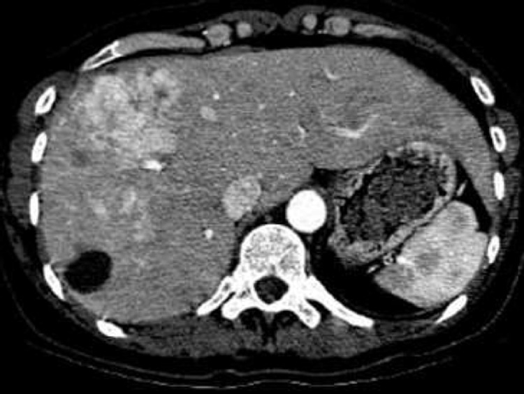
Example of an axial CT slice showing an enlarged human liver with inhomogeneous gray-value appearance due to pathological changes.

Different approaches to liver segmentation have been developed, and can be classified into three categories:

a) Fully automated approaches Many methods in this category utilize either a statistical shape model^7–10 or atlas-based approaches, like the methods presented by Linguraru et al.,¹¹ Furukawa et al.,¹² or Rikxoort et al.,¹³ to constrain the segmentation process. Building a liver model is challenging because of the large variation in liver shapes, and several alternatives to model-based methods were developed. For example, a rule-based segmentation method was presented by Schmidt et al.¹⁴ Chi et al.¹⁵ proposed a gradient vector flow snake framework, and a three-dimensional (3D) region-growing method was presented by Ruskó et al.¹⁶ Susomboon et al.¹⁷ suggested a combination of clustering, voxel classification and 2D region-growing for liver segmentation. A segmentation approach for multiphase contrast enhanced CT images was reported in Ref. 18.

b) Semiautomatic approaches A number of different semiautomatic liver segmentation methods can be found in the literature. A user-guided live wire approach for liver segmentation was presented by Schenk et al.¹⁹ Beck and Aurich²⁰ developed an interactive region-growing method. Several level set methods were utilized for liver segmentation. For example, two-dimensional (2D) level sets were utilized by Lee et al.²¹ Dawant et al.²² proposed a method based on 2D level sets with transversal contour initialization and a dynamic speed function. Another 3D level sets approach with orthogonal contour initialization was published by Wimmer et al.²³ Slagmolen et al.²⁴ used a nonrigid atlas matching method to segment the liver based on B-splines.

c) Manual approaches Manual contour drawing tools that are operated by the user can be found on many radiological workstations. The achievable segmentation accuracy solely depends on the skills and experience of the user. A major disadvantage of a manual liver segmentation is that it is a very time-consuming and tedious process.

Fully automated liver segmentation methods are desirable, but usually such approaches are likely to produce erroneous segmentations in a subset of clinically important cases. Thus, semiautomatic approaches are the most promising solution for routine clinical use. However, many of these approaches still require a considerable amount of user interaction. Using the live wire algorithm²⁵ for liver segmentation is one example: user interaction is required in each slice, even if an automated approach would succeed to deliver a correct segmentation result.

In this paper, we investigate the potential of a 3D semi-automated liver segmentation method which utilizes a virtual reality (VR) interface. The approach consists of two main processing steps. First, an initial liver segmentation is generated by means of a graph cut segmentation method. Second, 3D refinement methods allow the user to manipulate the segmentation result in 3D (e.g., surface of segmentation) to correct the initial segmentation, if needed. This processing step is facilitated by means of a VR-based user interface which offers stereoscopic visualization and six degrees of freedom (6 DOF) input devices. The rationale behind utilizing such a VR system is directly related to efficiency of human computer interaction required for correcting segmentations. Manipulating a surface (3D object) in a slice-by-slice (2D) manner is highly inefficient, error prone, and unintuitive. On the other hand, humans are experienced in manipulating objects in 3D and utilize stereopsis for this task. A VR system allows us to present the segmentation refinement problem in a natural (3D) environment—stereoscopic displays facilitate depth perception, and tracked input devices let the computer sense the 3D movements (6 DOF) of the users input device. In this work, we present an evaluation of our approach on twenty clinical liver CT data sets with three physicians, provide a comparison to a 2D editing approach, and draw conclusion regarding segmentation performance as well as feasibility and utility regarding clinical application.

II. METHODS

II.A. Outline of approach

The proposed approach to liver segmentation consists of two main stages: (a) initial graph cuts based segmentation and b) interactive segmentation refinement. Stage a) produces satisfactory results in many standard situations, but might fail locally in the cases were organs with similar gray-value appearance are adjacent or if liver gray-values are very inhomogeneous, for example. Possibly occurring segmentation errors can be corrected in stage (b) by manipulating (refining) the segmentation results of step (a) in 3D. Refinement can be done in two stages. First, automatically generated volume chunks can be added to removed from the segmentation result. Second, remaining errors can be corrected by manipulating/deforming the liver surface in 3D by means of various tools. Both of the refinement steps utilize a VR user interface to make the interaction with volume parts (chunks) or the object surface efficient and intuitive.

This two-stage approach to segmentation refinement allows reducing user interaction. The first refinement step is usually very fast, since it is bounded to volume chunks which are automatically generated by our algorithm. The majority of segmentation errors can be fixed or at least reduced by this approach. The second refinement step is based on the interactive deformation of the object surface and allows to arbitrarily modify the segmentation result. It may require more time compared to the first refinement stage, but typically the number of remaining segmentation errors is quite low.

The components of our approach are described in the following sections.

II.B. Graph cuts based segmentation

We use graph cuts²⁶ to generate an initial segmentation of the liver. For this purpose, we define a cost (energy) function as follows. Let P denote the set of voxels from the input volume data set V. To reduce computing time, only voxels with density values above −600 Hounsfield Units (HU) are considered as potentially belonging to the liver. The partition A = (A₁,…,A_p,…,A_|P|) with $A_p\in \{\text{``}\mathrm{obj}\text{''},\text{``}\mathrm{bkg}\text{''}\}$ can be used to represent the segmentation of P into liver/object (“obj”) and background (“bkg”) voxels. Let N be the set of unordered neighboring pairs {p, q} in set P according to a six-neighborhood relation. The cost of a given segmentation A is defined as

$$E\left(A\right)=B\left(A\right)+\lambda R\left(A\right),$$ (1)

where $R\left(A\right)={\sum }_{p\in P}{R}_p\left(A_p\right)$ takes into account region properties and $B(A)={\sum }_{\{p,q\}\in N}{B}_{p,q}{\delta }_{A_p\ne A_q}$ with ${\delta }_{A_p\ne A_q}=\{\begin{array}{cc}\multicolumn{1}{c}{1}& \hfill \mathit{if}{A}_p\ne A_q\hfill \\ \multicolumn{1}{c}{0}& \hfill \mathit{if}{A}_p=A_q\hfill \end{array}$ being boundary properties. The parameter λ in Eq. (1) with λ ≥ 0 allows to tradeoff the influence of the region versus boundary terms R(A) and B(A), respectively. Using the s-t cut algorithm, a partition (segmentation) A can be found which minimizes Eq. (1) (see Ref. 26 for details).

The region term R(A) specifies the costs of assigning a voxel to a label based on its gray-value similarity to object seed regions. For this purpose, user defined seed regions are utilized. Region cost R_p for a given voxel p is defined for labels “obj” and “bkg” as negative log-likelihoods

$$R_p(\text{``}\mathrm{obj}\text{''})=-\ln (\mathit{Pr}(I_p|\text{``}\mathrm{obj}\text{''}))=-\ln (e^{\frac{{(I_P-m_{\mathrm{obj}})}^2}{2{\sigma }_{\mathrm{obj}}^2}}),$$ (2)

and

$$R_p(\text{``}\mathrm{bjg}\text{''})=-\ln (\mathit{Pr}(I_p|\text{``}\mathrm{bkg}\text{''}))=-\ln (1-e^{\frac{{(I_P-m_{\mathrm{obj}})}^2}{2{\sigma }_{\mathrm{obj}}^2}}),$$ (3)

where m_obj and σ_obj represent the mean and standard deviation of the gray-values in the object seed region, and I_p denotes the gray-value of voxel p. In the above outlined approach, a simplification is made since liver gray-value appearance is usually not homogeneous, especially in contrast enhanced CT data due to vessels or tumors. However, this simplification works quite well in practice. Further, object seeds and the image boundaries are incorporated as hard constraints for object and background regions, respectively.

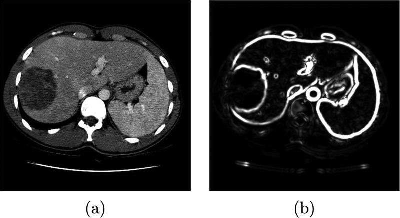
The basic idea behind the boundary term B(A) is to utilize a surfaceness measure, which allows to enhance weak edges and to suppress noise without blurring edges. First, to reduce the effect of unrelated structures on the gradient, the gray-value range of the image is truncated to a range between −150 and 200 HU. Second, the tensor of the Gaussian gradient S(x) is calculated for each voxel x. Image smoothing with a Gaussian with σ = 3.0 before gradient calculation reduces noise and restricts responses to structures of a certain scale. Third, to enhance weak edges and to reduce false responses, a 3D structure tensor W(x) is calculated (Fig. 2), similar as described in Ref. 27 for the 2D case. The structure tensor represents a second-moment matrix and is utilized to describe the predominant directions of the gradient in the neighborhood of a point. Fourth, a surfaceness measure t(W(x)) is calculated as described below. Let ${\mathbf{e}}_{1_{\mathbf{w}(\mathbf{x})}}$, ${\mathbf{e}}_{2_{\mathbf{w}(\mathbf{x})}}$, ${\mathbf{e}}_{3_{\mathbf{w}(\mathbf{x})}}$ be the eigenvectors and ${\lambda }_{1_{\mathbf{w}(\mathbf{x})}}\ge {\lambda }_{2_{\mathbf{w}(\mathbf{x})}}\ge {\lambda }_{3_{\mathbf{w}(\mathbf{x})}}$ the corresponding eigenvalues of W(x) at position x. If x is located on a plane-like structure, we can observe that ${\lambda }_1>>0$, ${\lambda }_2\approx 0$, and ${\lambda }_3\approx 0$. Thus, we define the surfaceness measure as

$$t(\mathbf{W}(\mathbf{x}))=\sqrt{{\lambda }_{1_{\mathbf{w}(\mathbf{x})}}-{\lambda }_{1_{\mathbf{w}(\mathbf{x})}}}.$$ (4)

In CT images, the liver is often separated only by weak boundaries, with higher gray level gradients present in close proximity. To take these circumstances into account, we utilize the following boundary cost term B_p,_q

$${B_{p,}}_q=\min \{\xi \left(t\left(\mathbf{W}\left({\mathbf{x}}_p\right)\right)\right),\xi \left(t\left(\mathbf{W}\left({\mathbf{x}}_q\right)\right)\right)\},$$ (5)

with the weighting function

$$\xi (t)=\{\begin{array}{cc}\multicolumn{1}{c}{1.0}& \hfill \mathrm{if}t<t_1\hfill \\ \multicolumn{1}{c}{0.001}& \hfill \mathrm{if}t>t_2\hfill \\ \multicolumn{1}{c}{(t-t_1)\frac{0.001-1}{t_2-t_1}+1}& \hfill \mathrm{otherwise}\hfill \end{array},$$ (6)

with t₁ = 2.0 and t₂ = 10.0. The idea behind this function is as follows. For gradient magnitudes t < t₁, we are sure that there are no boundaries. Thus, the costs for a cut have to be expensive. For gradient magnitudes t > t₂ we are sure that there are boundaries. Consequently, cutting has to be inexpensive, and all “real” boundaries are equally inexpensive. For gradient magnitudes between t₁ and t₂ uncertainty exists and a linear interpolation between cost values is used. With this approach we encourage the graph cut algorithm not to “blindly” follow the strongest boundaries, since the edges might belong to another nearby object. In addition, to force the graph cut segmentation to follow the ridges of the gradient magnitude, local nonmaximal responses along the image gradient direction are adjusted as follows: ${\xi }_{{\mathrm{non}}_{\mathrm{-}}\max }\left(t\right)=\min \{\xi \left(\mathrm{t}\right)+0.75,1\}$.

FIG. 2.

Boundary term calculation. (a) Original image. (b) Magnitude of the 3D structure tensor image W(x).

II.C. Volume-based segmentation refinement

In the first refinement step, the segmentation can be corrected by adding or removing volume chunks which are automatically derived from the previous graph cut stage. The chunks subdivide the graph cut segmentation result (object) as well as the background into disjunct subregions based on edge information. Thus, the initial segmentation result can be represented by chunks. Figure 3 illustrates the basic idea behind chunk-based segmentation refinement (CBR).

FIG. 3.

Example of chunk-based segmentation refinement (CBR). (a) Coronal slice of CT volume showing liver and adjacent vena cava inferior imaged with similar gray-values. The border between these two objects can be barely seen. (b) Initial graph cut result composed of chunks. (c) CBR result after two chunks have been removed—the leak has been successfully removed with a minimal amount of user interaction. Note that disconnected chunks are removed automatically. For (b) and (c) a point-rendering method is used for visualization of volume chunks.

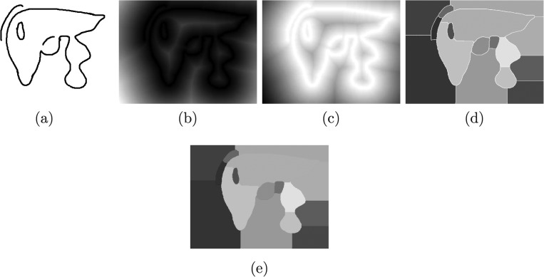
Volume chunks are generated by utilizing a distance transformation and watershed segmentation.²⁸ The processing steps are illustrated in Fig. 4 and described below. First, with the threshold operation N(t(W(x))) > 10, a binary volume is generated which represents boundaries/surfaces voxels, where N denotes the nonmaximal suppression operator.²⁸ In this context, the selection of the threshold (10 in our case) is not very critical. Since the method can handle gaps in the edge scene, the threshold can be set very conservative. Thus, it should be chosen such that background noise is suppressed completely. Second, the resulting volume is merged with the boundary from the graph cut segmentation by using a logical “or” operation, and a distance transformation²⁹ is calculated. Inverting this distance map results in an image that can be interpreted as a height map suitable for watershed segmentation. Due to the discrete nature of digital images, a number of small (catchment) basins arise. To avoid oversegmentation, all small local minima resulting from this quantization noise in the distance map are eliminated using the H-Minima algorithm.³⁰ After running a watershed segmentation on the height map, the binary boundary scene is almost completely segmented but the original boundaries are left over. Thus, boundary voxels are merged with the neighboring chunks containing the most similar bordering voxels.

FIG. 4.

2D illustration of the volume chunk generation process described in Sec. II C. (a) Binary boundary scene. (b) Distance map. (c) Height map. (d) Initial watershed segmentation, (e) Watershed segmentation with assigned boundaries.

The proposed method has some interesting properties (Fig. 4). First, it naturally handles broken boundaries. It closes even large gaps and groups pixels together similar to the medial axis transformation. This grouping is very intuitive and similar to human perception.³¹ It is well suited to split up an object at a constriction (e.g., two connected neighboring objects). Second, using initial boundary information, the initial segmentation is subdivided, which can be used to exclude parts like for example the vena cava inferior in Fig. 3.

CBR can be done very efficiently, since the user has to select/deselect predefined chunks, which does not require a detailed manual border delineation. However, this step requires tools for interactive data (CT information, segmentation, and chunks) visualization and interaction. For this purpose, a hybrid user interface was developed which is described in Sec. II E.

During the process of adding and removing volume chunks, holes within the object may be formed, or some chunks may become disconnected from the object to be segmented. Thus, to facilitate the chunk-based refinement, an adjacency-graph-based data structure is utilized in combination with an algorithm to close holes and remove disconnected chunks automatically.

II.D. Mesh-based segmentation refinement

After chunk-based segmentation refinement, the set of selected chunks is converted to a deformable mesh model to enable surface-based segmentation refinement. This is done by shrinking a coarse initial simplex mesh³² created using the Wrapper algorithm described in Ref. 33 to extract an initial triangular mesh (Ref. 34) based on a downsampled version (64 × 64 × 64 voxels) of the segmentation. The triangular mesh is converted to a simplex mesh using the duality between simplex meshes and triangular meshes.³² Subsequent mesh fitting is done by performing simplex mesh iterations

$${\mathbf{P}}_i^{t+1}=(1-\gamma )({\mathbf{P}}_i^t-{\mathbf{P}}_i^{t-1})+{\alpha }_i{\overrightarrow{F}}_{\mathrm{innt}}(i)+{\beta }_i{\overrightarrow{F}}_{\mathrm{ext}}(i),$$ (7)

with α_i = 0.3, β_i = 0.17, and γ = 0.9 until convergence. During this process, external forces ${\overrightarrow{F}}_{\mathrm{ext}}(i)$ for the simplex mesh deformation are calculated based on a 3D Bresenham traversal of the segmentation volume, while internal forces ${\overrightarrow{F}}_{\mathrm{int}}(i)$ avoid mesh degeneration. In addition, automatic mesh restructuring based on polygon merge and polygon split operations is performed by evaluating a number of mesh quality criteria. Criteria include discrete approximation of the mean curvature, polygon elongation and surface welding at edges. The mesh fitting process typically increases the number of vertices and polygons. However, this only happens in regions where segmentation surface properties require a more complex representation. The mesh quality criteria are set to values which ensure that each mesh vertex is closer than half a voxel diameter to the segmentation boundary. This results in surfaces accurately representing the segmentation, while keeping model complexity sufficiently low for real-time deformation in the mesh-based refinement step.

Surface-based segmentation refinement is an iterative process consisting of the following three steps:

• 1.Surface Inspection: The user locates errors in the surface model by comparing raw CT data with the boundary of the segmentation surface. This is supported by a variety of visualization modes for the mesh (e.g., rendering the opaque model either colored or textured with CT data), which helps to identify segmentation errors. In addition, a textured cutting plane showing original CT data can be arbitrarily placed in the data set volume. Clipping the model at the cutting plane while highlighting the contour on the plane greatly helps to identify segmentation errors.
• 2.Error Marking: Regions of the surface model that were found erroneous during the inspection step are marked red by means of painting tool to enable further processing. In addition, surface parts can be marked in green (default setting), which makes them immutable to prevent accidental modifications.
• 3.Error Correction: Regions marked in red are corrected by utilizing a range of interactive tools.

The above described steps are repeated until the desired result has been achieved. Several tools are available to the user to perform segmentation refinement:

Vertex Drag Tool—The vertex drag tool is the simplest mesh editing tool. It allows the user to manipulate a simplex mesh by moving individual vertices.

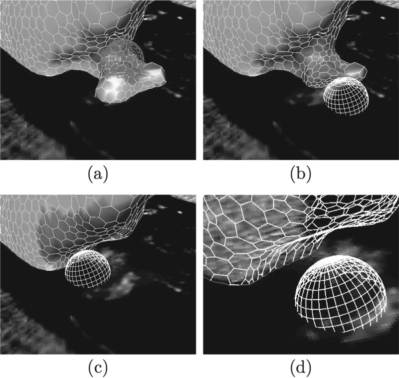
Sphere Tool—This refinement tool is based on the idea of using a geometrical shape (sphere of user-defined radius) as form element in the sense of sculpting tool. It can be interactively placed in the data set in 3D. Sphere deformation at a specific 3D position causes object surface parts located within the sphere shape to be successively moved outwards on the shortest possible path. Therefore, placing the sphere tool so that most parts of it are outside the object causes its surface to move inwards, while bulging behavior is achieved by placing the sphere mostly inside the object. Moving the input device while the deformation tool is active causes the tool to respond just as if one was deforming a piece of clay using a real world modeling tool. External simplex mesh forces ${\overrightarrow{F}}_{\mathrm{ext}}$ are calculated for all mesh vertices located inside the sphere visualized as a wire frame model. In order to deliver greater flexibility in terms of the shapes that can be modeled, automatic simplex mesh restructuring is performed throughout the deformation process. Figure 5 presents an example, showing the tool being used to remove a segmentation error.

FIG. 5.

Utilization of the sphere deformation tool to correct a leak. (a) Marking the region containing the segmentation error. (b) Refinement using the sphere tool. (c) After applying the sphere tool, the error is corrected. (d) The corrected region in wire frame mode highlighting the mesh contour.

Plane Tool—This tool is similar to the Sphere Tool, except that a disk shape is utilized as form element.

Smoothing Tool—The interactive mesh smoothing can be used to improve a mesh reconstructed from a noisy segmentation. This is achieved by setting all external forces ${\overrightarrow{F}}_{\mathrm{ext}}$ of the selected region to zero and automatic mesh restructuring operations are utilized to merge polygons.

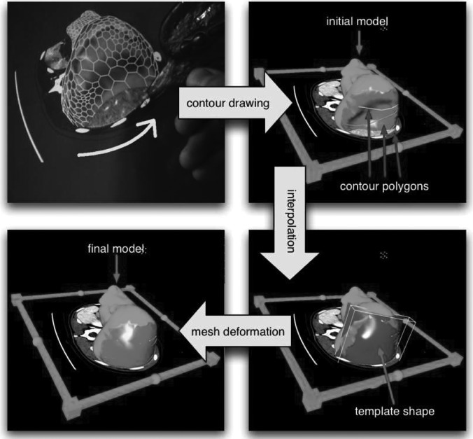
Template Shape Tool—Direct surface editing is most efficient for small segmentation errors. If larger surface regions are affected, a semiautomatic template shape tool can be utilized (Fig. 6). The developed tool is based on the idea to specify a three-dimensional surface—the template shape—which locally models the erroneous region correctly. The template shape has to be specified by the user in a first interactive stage, while the second stage, deformation towards the template, is automatic. Using the template shape tool starts by marking all parts of the surface to be corrected (Fig. 6). Next, a small number of contour polygonal lines have to be drawn utilizing the textured cutting plane. The template shape is then computed by interpolating the vertices of the polygonal lines using thin plate splines.³⁵ In the automatic stage, the template shape tool involves force calculation towards the template.

FIG. 6.

Segmentation refinement using the template shape tool. First, contours are drawn on the cutting plane showing context data, leading to a rough sketch of the erroneous region in form of polygonal lines. Usually a small number of contours is sufficient. In the next stage, the contours are interpolated using a spline surface to form the template shape. In this stage, contours can still be edited, thereby updating the template. Finally, the model automatically deforms towards the template shape.

II.E. Hybrid desktop/virtual reality user interface

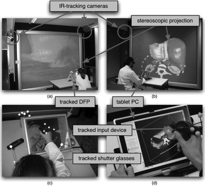
The user interface is of great importance for the utility of the segmentation refinement tools described in Secs. II C and II D. The proposed segmentation refinement process requires user interaction for two different tasks. In the first refinement stage (CBR), the user has to check the segmentation and refine it by adding or removing chunks, if necessary. This requires navigation tasks like viewing the initial segmentation from different sides/perspectives and placement of the cutting plane inside the data set. Second, 3D surface (mesh) manipulation has to be performed, which is a task clearly suggesting in place 3D interaction. To facilitate the above outlined tasks, we utilize a hybrid user interface (Fig. 7) which consists of a desktop part for 2D interaction and a VR part, offering stereoscopic visualization of 3D objects from the user’s viewpoint. In this way, 3D interaction techniques can be offered for tasks like segmentation refinement, while advantages of a conventional desktop setup like higher screen resolution and higher input precision are preserved. For the VR system part, a stereoscopic back-projection system was used. The user wears shutter glasses, and an optical tracking system is utilized to track the user’s head to enable a realistic visualization of 3D objects. The desktop part of the system consists of a PC equipped with a tracked digital flat panel (DFP) screen [Figs. 7(a) and 7(c)]. Alternatively, a tablet PC can be utilized [Figs. 7(b) and 7(d)]. The VR and desktop systems run separate applications which share and synchronize the segmentation data over a network connection.

FIG. 7.

Hybrid system setup. The VR setup consists of a stereoscopic projection screen and an optical tracking system to track the user’s head and the input device (a) and (b). For the 2D setup, a touchscreen or an arbitrary tracked screen can be placed in front of the user. (c) In case of a tracked screen mouse input is calculated by utilizing data from the tracking system. (d) Alternatively, a touch screen or a tablet PC can be used directly.

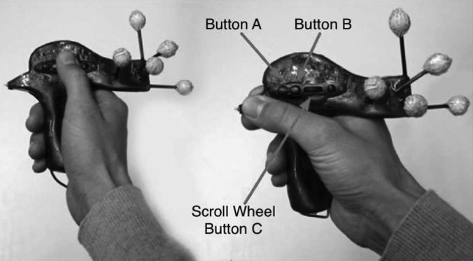
The utilized input device which is tracked in six degrees of freedom facilitates 2D as well as 3D interaction (Fig. 8). It supports coarse cutting plane placement (3D), precision tasks like mesh editing at vertex level (2D and 3D), and acting as a mouse replacement (2D) at the same time.

FIG. 8.

Input device utilized for 2D and 3D interaction. Various buttons are used to trigger interaction. The device is also equipped with tracking targets for optical tracking.

III. EXPERIMENTAL METHODS

III.A. Image data

Twenty routinely acquired multidetector CT data sets of potential liver surgery patients were collected. For each patient, the CT volume depicted the portal venous phase. The data sets show a large variation in anatomy, pathology, and image quality (e.g., tumors, abnormal shape due to previous resection, motion artifacts,...). The sizes of data sets ranged from 512 × 512 × 75 to 512 × 512 × 206 voxels with intraslice resolutions between 0.549 and 0.799 mm and a median of 0.703 mm. The interslice distances were between 1.0 and 4.0 mm, with the majority at 2 mm or smaller (median: 2 mm). None of the evaluation data sets has been used for the development of algorithms.

III.B. Independent reference standard

For each of the 20 test data sets, a physician traced the outline of the liver using a live wire²⁵ tool. Note that the reference segmentation excludes the vena cava inferior, which is frequently partly or fully surrounded by liver tissue. Excluding the vena cava inferior is important, because it is an anatomical feature of relevance for surgical resection planning or IGRT simulation.

III.C. Quantitative indices

For segmentation error assessment, surface- and volume-based measures are used. Let V_S and V_r be binary volume data sets describing the segmentation result and the reference segmentation, respectively. Corresponding surfaces will be denoted as S and R. The distance d(x, A) between a point x and a surface A is defined as $d(x,A)=\underset{x\text{'}\in A}{\min }\Vert x-x\text{'}\Vert$. In the following, surface-based error measures were used: the mean distance d_mean(S, R) = [I(S, R) + I(R, S)]/[|S| + |R|] with $I(A,B)={\int }_{x\in A}d(x,B)\mathit{dx}$ and the Hausdorff distance $d_H(S,R)=\max (\underset{x\in S}{\max }\{d(x,R)\},\underset{x\in S}{\max }\{d(x,S)\})$. To measure the volume error, the overlap v_abs(V_S,V_R) = |V_S/V_R|  + |V_r/V_s| and relative overlap error $v_r(V_S,V_R)=1-2\mathrm{|}{V}_S\cap V_R\mathrm{|}\mathrm{/}\left[\right|V_S|+|V_R\left|\right]$ were used. For depicting the distributions of error and time measurements, notched box-and-whisker plots were utilized. The box has lines at the lower quartile, median, and upper quartile values. The whiskers show the extent of the rest of the data. Outliers are displayed by a “+” symbol. Notches represent a robust estimate of the uncertainty about the medians for box to box comparison (significance level of 0.05).

III.D. Experimental setup

The initial seed region specification were provided and the graph cut segmentation as well as the chunk generation was calculated. Usually, the selection of the seed region is not very critical and can be performed by an assistant. Thus, all medical experts who took part in the evaluation had the same start conditions. The experts were required to generate high quality segmentations that clearly show anatomical landmarks like the vena cava inferior. Based on the initial graph cut segmentation and chunk generation results, three physicians were asked to perform the following interaction steps: (a) CBR and (b) mesh-based refinement (MBR). All two steps were performed using the hybrid desktop/VR user interface. Intermediate results and task completion times were recorded. Data sets were presented in random order to experts. Prior to evaluation, all experts were introduced to the system by an instructor. Afterwards, users were allowed to explore the system using data sets other than the test data sets. After that two-step training phase, which lasted for 1 h, experts were asked to segment the liver in the twenty test data sets. All experts were using our system for the first time. In the following, the initial graph cut segmentation errors are reported too and will be denoted as “initial”.

For a comparison with standard 2D (i.e., slice-by-slice) segmentation refinement tools, a fourth expert (expert 4), who had not seen or worked with the test data before, was asked to refine the initial graph cut segmentation by utilizing 3D Slicer, a state of the art open source software package for visualization and medical image computing.³⁶ The results obtained with this method will be denoted as “2D.” Prior to refining all twenty initial segmentations, expert 4 was trained on the 2D tools in the same manner as the other experts on the 3D system.

IV. RESULTS

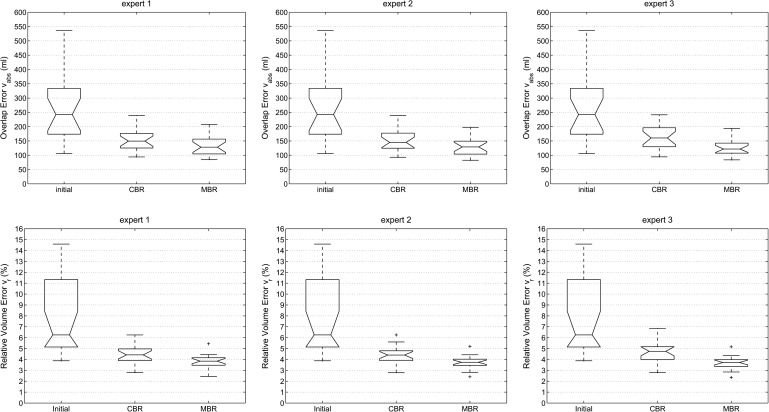
Box-and-whisker plots of the mean distance error d_mean and the corresponding volume overlap errors v_abs and v_r for all three experts (proposed method) and different processing stages are shown in Figs. 9 and 10, respectively. All three error metrics show a decrease of error with progressing refinement stages. Relating d_mean to the median voxel dimensions leads to an average error of one to two voxels. In addition, Table I summarizes volume-based and Table II distance-based error measurements for the proposed and 2D approach, and Fig. 11 provides a side-by-side comparison of final (i.e., after MBR) error indices with the 2D refinement approach.

FIG. 9.

Distance error d_mean for all three experts and different processing stages of the segmentation refinement process; initial: error after initial graph cut segmentation; CBR: error after chunk-based refinement; MBR: final result after mesh-based refinement.

FIG. 10.

Volume-based error indices v_abs and v_r for all three experts and different processing stages of the segmentation refinement process; initial: error after initial graph cut segmentation; CBR: error after chunk-based refinement; MBR: final result after mesh-based refinement.

TABLE I.

Volume error.

		Mean ± std	Mean ± std	Mean ± std	Mean ± std
Initial	vabs (ml)	283.5 ± 152.5
	vr (%)	7.90 ± 3.62
		Expert 1	Expert 2	Expert 3	2D
CBR	vabs (ml)	154.2 ± 40.6	153.6 ± 41.0	163.3 ± 44.7	N/A
	vr (%)	4.46 ± 0.86	4.43 ± 0.86	4.71 ± 0.96	N/A
MBR/final	vabs (ml)	131.9 ± 32.5	128.4 ± 30.0	126.2 ± 28.2	138.6 ± 38.7
	vr (%)	3.81 ± 0.63	3.72 ± 0.59	3.69 ± 0.60	4.00 ± 0.74

TABLE II.

Distance error.

		Mean ± std	Mean ± std	Mean ± std	Mean ± std
		(mm)	(mm)	(mm)	(mm)
initial	dmean	3.14 ± 1.65
		Expert 1	Expert 2	Expert 3	2D
CBR	dmean	1.43 ± 0.31	1.42 ± 0.32	1.51 ± 0.32	N/A
MBR/final	dmean	1.22 ± 0.24	1.18 ±0.21	1.17 ± 0.21	1.27 ± 0.37
initial	dH	59.53 ± 30.01
		Expert 1	Expert 2	Expert 3
CBR	dH	29.09 ± 7.45	28.07 ± 8.25	31.35 ± 8.80	N/A
MBR/final	dH	21.66 ± 7.00	22.26 ± 6.55	21.81 ± 5.96	30.22 ± 13.63

FIG. 11.

Comparison of segmentation refinement results between the proposed method (expert 1–expert 3) and 2D-based segmentation refinement. (a) Mean distance error d_mean. (b) Overlap error v_abs. (c) Relative volume error V_r.

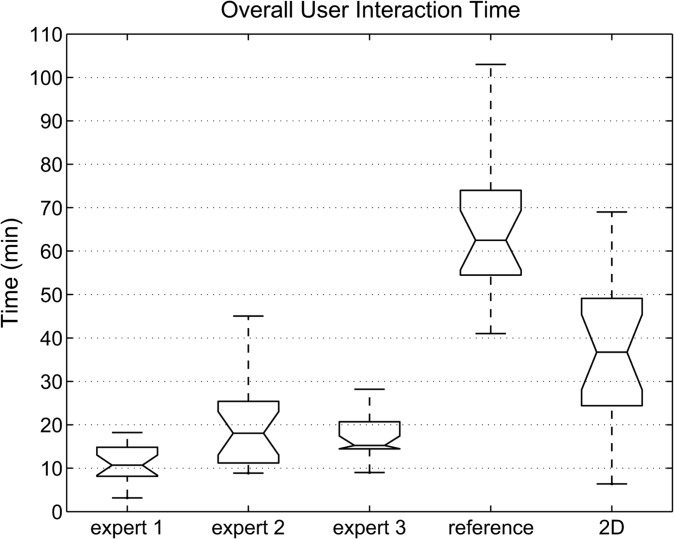
Table III and Fig. 12 show the overall interaction time required when utilizing the proposed (expert 1–expert 3) and standard 2D refinement approaches. For the proposed method, the times required for performing individual refinement steps are also listed in Table III. In addition, the fraction of time required for MBR in areas of vessel entrance or exit, which is denoted as “refinement of vessels”, is given. Similarly, the time spent on refining such areas with the 2D tool was recorded and is summarized in Table III. Handling vessels is a frequently occurring refinement step which accounts for quite a large portion of the required user interaction. Furthermore, the time required by the radiologist to generate the reference segmentation using the live wire tools is shown for comparison in Table III and Fig. 12, respectively. On average, the three experts that were utilizing the proposed 3D approach required 11.6 s for refinement per axial CT slice that depicted liver tissue. In comparison, 47.7 and 18.7 s were required per liver slice for the live wire and 2D approach, respectively. Comparisons between MBR results and reference segmentations are shown in Figs. 13 and 14.

TABLE III.

Interaction time.

	Mean ± std	Mean ± std	Mean ± std	Mean ± std	Mean ± std
	(min)	(min)	(min)	(min)	(min)
	Expert 1	Expert 2	Expert 3	Reference	2D
CBR	3.2 ± 1.3	5.9 ± 2.7	2.9 ± 1.4	N/A	N/A
MBR	7.9 ± 3.8	13.8 ± 8.7	14.3 ± 5.8	N/A	N/A
Overall	11.1 ± 4.5	19.7 ± 9.9	17.2 ± 5.7	70.1 ± 28.8	38.3 ± 20.2
Refinement of vessels	2.9 ± 2.3	5.5 ± 4.7	4.1 ± 3.3	N/A	19.82 ± 14.03

FIG. 12.

User interaction time needed for the segmentation of the 20 test cases. The interaction times required for generating the reference segmentation using a live wire and 2D tool are shown for comparison.

FIG. 13.

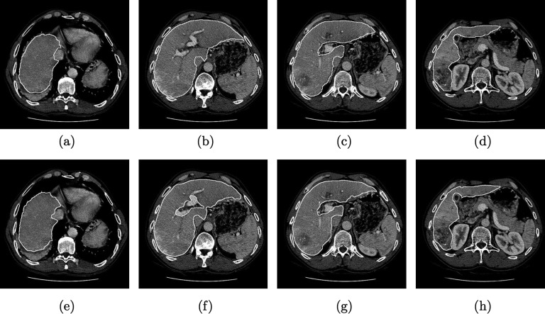
Example showing segmented axial CT slices of a data set. (a)–(d) Live wire reference segmentation. (e)–(h) Result after MBR performed by expert 3. Differences in the region of portal vein entrance are clearly visible.

FIG. 14.

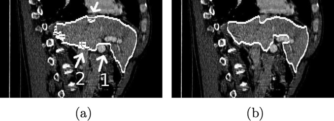
Comparison between (a) reference segmentation and (b) MBR segmentation result (expert 3) in a sagittal slice. The area of portal vein entrance is marked with a white arrow and the number one in (a), and regions close to the vena cava inferior are marked with arrows and the number two. Axial images of the same data set are depicted in Fig. 13.

An analysis of variance (ANOVA) test was performed to verify the impression gained from Fig. 10, that the mean relative overlap error mean(v_r) for each expert is not significantly different after MBR. A p-value of p = 0.82 confirms the ANOVA null hypothesis that all relative overlap errors are drawn from populations with the same mean. This was also the case for the other error metrics: v_abs (p = 0.84), d_mean (p = 0.89), and d_H (p = 0.96). In contrast, the time required for user interaction by the three experts was found to be significantly different (p = 0.0009).

Table IV summarizes the number of unchanged, changed, added, and removed volume chunks during CBR. On average, six or less chunks were changed during CBR by the three experts. Despite the low average number of chunks changed, the achievable improvement in segmentation performance is quite large (Figs. 9 and 10).

TABLE IV.

Chunk refinement statistic.

		Expert 1	Expert 2	Expert 3
Unchanged	Mean ± std	24.05 ± 9.28	23.60 ± 9.56	23.85 ± 9.96
	Median	24.00	23.50	24.00
Changed	Mean ± std	5.80 ± 4.42	6.00 ± 3.96	5.00 ± 4.05
	Median	6.00	6.00	4.50
Added	Mean ± std	2.20 ± 2.73	2.50 ± 2.52	1.75 ± 2.38
	Median	1.50	2.00	1.00
Removed	Mean ± std	3.60 ± 3.73	3.50 ± 3.63	3.25 ± 3.65
	Median	3.00	3.00	2.50

To compare the proposed 3D with the standard 2D approach, ANOVA tests were performed. The utilized error indices V_r (p = 0.4602), v_abs (p = 0.6357), d_mean (p = 0.6926), and d_H (p = 0.0522) were not found to be statistically significant different at significance level of 0.05. In contrast, the overall time required for the 2D refinement was found to be significantly larger (p = 0.000098). An example of 2D and 3D refinement results is depicted in Fig. 15. In addition, the time required for refinement with the 2D tool was found to be statistically significant lower (p = 6.34 × 10⁻⁷) when compared to the live wire tool utilized for generating the reference segmentation.

FIG. 15.

Comparison of segmentation refinement approaches. (a) Initial graph cut segmentation, (b) Corresponding 2D (slice-by-slice) segmentation refinement result. (c) Corresponding 3D (after MBR) segmentation refinement result generated by expert 1.

V. DISCUSSION

In this work we investigated a new VR-based approach for interactive segmentation of livers in volumetric CT data. The main idea behind this approach is that the user interacts with volume chunks and/or surfaces instead of 2D contours in cross-sectional images (i.e., slice-by-slice). To facilitate this process, a VR-based user interface was utilized which enables stereoscopic visualization and manipulation of virtual objects in 6 DOF. For our experiments, the user interface was implemented in a general purpose VR environment with a large back-projection wall, and many components of this setup were custom-made. For clinical application, this setup can be further optimized. For example, a desktop version of our system, which uses consumer active stereo display technology (e.g., NVIDIA 3D Vision, nvidia Corporation, Santa Clara, California), can be built for the price of a radiology workstation. Recent trends in consumer electronics (3D TVs) and interactive entertainment (video games) industry suggest, that VR systems are becoming mainstream. As a consequence, VR technology will become cheaper and standardized. Thus, we expect that the utilization of such VR technology for medical applications will steadily increase over the coming years.

The three physicians that participated in our study had not used our system before and had no experience with VR systems in general. Despite the short introduction phase of 1 h, all three experts were able to produce segmentations with low error rates, that showed no statistically significant different error indices amongst each other. The produced segmentations were well suited for the evaluation of liver cancer treatment options (e.g., surgery, radiation treatment, etc.).

Compared to the live wire based slice-by-slice segementation approach (labeled reference in Table III and Fig. 12), the achieved time savings range between 72% and 85% on average per CT scan, depending on the expert performing the refinement. Average time savings of our method ranged between 49% and 71% per CT scan, compared to 2D segmentation refinement. The differences in user interaction time required by the three experts (Table III and Fig. 12) was statistically significant and can be explained as follows. The proposed 3D system offers several tools designed to effectively correct different types of segmentation errors. Consequently, a suboptimal tool selection or refinement strategy will result in a longer interaction time. Since all experts were using the segmentation system for the first time, some experts might benefit from a longer training phase, allowing them to fully get used to the refinement tools and to develop efficient refinement strategies. Thus, it is very likely that after an extended learning phase, an average interaction time of 11 min per liver or less, as measured for expert 1, can be routinely achieved. Our results suggest a quick amortization of the time spent on training of users.

Figures 13 and 14 depict the reference and the segmentation results (after MBR) produced by expert 3 for one data set. For this case, a relative overlap error v_r of 4.4% was achieved by expert 3. In this case, v_r is higher than the average (Table I). Major differences can be noticed in areas where vessels enter/leave (e.g, portal vein) or are close to the liver (e.g., vena cava inferior), which is clearly visible in Figs. 13(b) and 13(f), and 14. In such regions, no accepted criteria for defining liver boundaries exist.

For all utilized error indices, the 2D approach has higher values for mean and standard deviation (Tables I and II). In a statistical analysis, these differences were not found to be significant. In contrast, time required for user interaction was significantly lower for the 3D method. Figure 15 depicts a comparison of segmentation refinement results between the 2D and 3D approach. In this case, the initial graph cut segmentation of the liver was not correct and included parts of the inferior vena cava, besides other errors (e.g., excluded tumor). The 3D refinement result shows a smooth and very accurate boundary in this region, whereas the 2D refinement result has inconsistencies between slices (zigzag line). This example demonstrates the advantages of 3D segmentation refinement: a) inconsistencies between slices are avoided and b) refinement can be done faster, because a surface is manipulated instead of a set of 2D contours.

For a comparison of our approach with other methods, we applied it to all ten test CT data sets collected for the MICCAI 2007 liver segmentation competition.^37,38 Segmentation results were sent to the organizers, which then provided evaluation results (error metrics) in return. Detailed rules for handling of vessels were provided; vessel were counted as internal if they were completely surrounded by liver tissue in the transversal view or were inside the convex hull enclosing liver tissue. The average results achieved on the test cases were as follows: overlap error 5.2%, relative absolute volume difference (vol. diff.) 1.0%, average symmetric surface distance (avg. diff.) 0.8 mm, root mean square (RMS) symmetric surface distance 1.4 mm, and maximum symmetric surface distance 15.7 mm. Based on these performance metrics, a total score of 82 was calculated. In comparison, the score after CBR was 74. A larger total score represents a more accurate segmentation result.³⁸ The expert who was using the system had already some experience with the proposed segmentation system. For the CBR step, 58 s were required on average, and the MBR step took 5 min on average. Based on the comparison published by Heimann et al.,³⁸ out of ten automated segmentation approaches, a shape-constrained segmentation approach based on a heuristic intensity model achieved the highest total score of 77. Thus, with our approach, more accurate segmentations can be produced than with fully automated liver segmentation approaches. The highest total score of other semiautomatic liver segmentation approaches was 77.³⁸ The liver segmentation performance comparison (competition) is ongoing, and the reader is referred to MICCAI 2007 liver segmentation competition website³⁷ for more recent scores. However, in some cases, a meaningful/fair comparison with methods not included in the original study presented by Heimann et al.³⁸ is not possible, because methods or improvements to prior published methods have not been published and/or details about algorithms, computing time or user interaction, etc. are not available.

For the study presented in Sec. IV, experts were asked to produce high quality liver segmentations. However, for some clinical applications, a less detailed segmentation might be sufficient (e.g., omitted MBR step). Thus, the user can find the optimal trade-off between segmentation quality and interaction time for each application. This is also clearly demonstrated by the time needed to segment the ten data sets for the liver segmentation competition, where a lower level of detail was required. In this case, the time for refinement was approximately half the time needed by expert 1.

VI. CONCLUSIONS

A VR-based liver segmentation concept was presented and evaluated. Experiments on twenty routinely acquired contrast enhanced CT data sets showed that all three participating physicians were able to produce liver segmentations with low error indices that were well suitable for assessment of liver cancer treatment options. Average user interaction time savings of up to 85% and 71% were achieved, compared to a standard semiautomatic live wire and 2D segmentation refinement approach, respectively.

The developed segmentation refinement method represents a new paradigm for the utilization of stereoscopic display devices and advanced interaction concepts in the context of segmentation of volumetric medical image data. The concept is not limited to a specific organ or modality. In the future, we plan to adapt our approach to other application domains.

REFERENCES

- 1. The World Health Report, World Health Organization http://www.who.int/whr/2004/en
- 2.Burak K. W. and Bathe O. F., “Is surgical resection still the treatment of choice for early hepato-cellular carcinoma?,” J. Surg. Oncol. 104 (1), 1–2 (2011). 10.1002/jso.21765 [DOI] [PubMed] [Google Scholar]
- 3.Llovet J. M., Schwartz M., and Mazzaferro V., “Resection and liver transplantation for hepato-cellular carcinoma,” Semin Liver Dis. 25 (2), 181–200 (2005). 10.1055/s-2005-871198 [DOI] [PubMed] [Google Scholar]
- 4.Lamade W., Glombitza G., Fischer L., Chiu P., Cardenas C. E., Thorn M., Meinzer H.-P., Grenacher L., Bauer H., Lehnert T., and Herfarth C., “The impact of 3-dimensional reconstructions on operation planning in liver surgery,” Arch. Surg. 135 (11), 1256–1261 (2000). 10.1001/archsurg.135.11.1256 [DOI] [PubMed] [Google Scholar]
- 5.Selle D., Preim B., Schenk A., and Peitgen H.-O., “Analysis of vasculature for liver surgical planning,” IEEE Trans. Med. Imaging 21 (11), 1344–1357 (2002). 10.1109/TMI.2002.801166 [DOI] [PubMed] [Google Scholar]
- 6.Lang H., Radtke A., Liu C., Frühauf N. R., Peitgen H.-O., and Broelsch C. E., “Extended left hepatectomy-modified operation planning based on three-dimensional visualization of liver anatomy,” Langenbecks Arch. Surg. 389, 306–310 (2004). 10.1007/s00423-003-0441-z [DOI] [PubMed] [Google Scholar]
- 7.Kainmüller D., Lange T., and Lamecker H., “Shape constrained automatic segmentation of the liver based on a heuristic intensity model,” in MICCAI 2007 Workshop proceedings of 3-D Segmentation Clinic: A Grand Challenge, edited by Heimann T., Styner M., and van Ginneken B. (Brisbane, Australia, 2007), pp. 109–116 [Google Scholar]
- 8.Heimann T., Meinzer H. P., and Wolf I., “A statistical deformable model for the segmentation of liver CT volumes,” in MICCAI 2007 Workshop proceedings of 3-D Segmentation Clinic: A Grand Challenge, edited by Heimann T., Styner M., and van Ginneken B. (Brisbane, Australia, 2007), pp. 161–166 [Google Scholar]
- 9.Seghers D., Slagmolen P., Lambelin Y., Hermans J., Loeckx D., Maes F., and Suetens P., “Landmark based liver segmentation using local shape and local intensity models,” in MICCAI 2007 Workshop proceedings of 3-D Segmentation Clinic: A Grand Challenge, edited by Heimann T., Styner M., and van Ginneken B. (Brisbane, Australia, 2007), pp. 135–142 [Google Scholar]
- 10.Saddi K. A., Rousson M., Chefd’hotel C., and Cheriet F., “Global-to-local shape matching for liver segmentation in CT imaging,” in MICCAI 2007 Workshop proceedings of 3-D Segmentation Clinic: A Grand Challenge, edited by Heimann T., Styner M., and van Ginneken B. (Brisbane, Australia, 2007), pp. 207–214 [Google Scholar]
- 11.Linguraru M. G., Sandberg J. K., Li Z., Shah F., and Summers R., “Automated segmentation and quantification of liver and spleen from CT images using normalized probabilistic atlases and enhancement estimation,” Med. Phys. 37 (2), 771–783 (2010). 10.1118/1.3284530 [DOI] [PMC free article] [PubMed] [Google Scholar]
- 12.Furukawa D. , Shimizu A. , and Kobatake H. , “Automatic liver segmentation based on maximum a posterior probability estimation and level set method,” in MICCAI 2007 Workshop proceedings of 3-D Segmentation Clinic: A Grand Challenge , edited by Heimann T. , Styner M. , and van Ginneken B. (Brisbane, Australia, 2007), pp. 117–124 [Google Scholar]
- 13.van Rikxoort E., Arzhaeva Y., and van Ginneken B., “Automatic segmentation of the liver in com puted tomography scans with voxel classification and atlas matching,” in MICCAI 2007 Workshop proceedings of 3-D Segmentation Clinic: A Grand Challenge, edited by Heimann T., Styner M., and van Ginneken B. (Brisbane, Australia, 2007), pp. 101–108 [Google Scholar]
- 14.Schmidt G., Athelogou M. A., Schönmeyer R., Korn R., and Binnig G., “Cognition network technology for a fully automated 3-D segmentation of liver,” in MICCAI 2007 Workshop proceedings of 3-D Segmentation Clinic: A Grand Challenge, edited by Heimann T., Styner M., and van Ginneken B. (Brisbane, Australia, 2007), pp. 125–133 [Google Scholar]
- 15.Chi Y., Cashman P. M. M., Bello F., and Kitney R. I., “A discussion on the evaluation of a new automatic liver volume segmentation method for specified CT image datasets,” in MICCAI 2007 Workshop proceedings of 3-D Segmentation Clinic: A Grand Challenge, edited by Heimann T., Styner M., and van Ginneken B. (Brisbane, Australia, 2007), pp. 167–175 [Google Scholar]
- 16.Ruskó L., Bekes G., Németh G., and Fidrich M., “Fully automatic liver segmentation for contrast- enhanced CT images,” in MICCAI 2007 Workshop proceedings of 3-D Segmentation Clinic: A Grand Challenge, edited by Heimann T., Styner M., and van Ginneken B. (Brisbane, Australia, 2007), pp. 143–140 [Google Scholar]
- 17.Susomboon R., Raicu D. S., and Furst J., “A hybrid approach for liver segmentation,” in MICCAI 2007 Workshop proceedings of 3-D Segmentation Clinic: A Grand Challenge, edited by Heimann T., Styner M., and van Ginneken B. (Brisbane, Australia, 2007), pp. 151–160 [Google Scholar]
- 18.Ruskó L., Bekes G., and Fidrich M., “Automatic segmentation of the liver from multi- and single-phase contrast-enhanced CT images,” Med. Image Anal. 13 (6), 871–882 (2009). 10.1016/j.media.2009.07.009 [DOI] [PubMed] [Google Scholar]
- 19.Schenk A., Prause G. P. M., and Peitgen H. O., “Efficient semiautomatic segmentation of 3D objects in medical images,” in Medical Image Computing and Computer-Assisted Intervention — MICCAI 2000, Lecture Notes in Computer Science, (Springer, Berlin/Heidelberg, 2000), Vol. 1935, pp. 186–195 [Google Scholar]
- 20.Beck A. and Aurich V., “Tux-a semiautomatic liver segmentation system,” in MICCAI 2007 Workshop proceedings of 3-D Segmentation Clinic: A Grand Challenge, edited by Heimann T., Styner M., and van Ginneken B. (Brisbane, Australia, 2007), pp. 225–234 [Google Scholar]
- 21.Lee J., Kim N., Lee H., Seo J. B., Won H. J., Shin Y. M., and Shin Y. G., “Efficient liver segmentation exploiting level-set speed images with 2.5D shape propagation,” in MICCAI 2007 Workshop proceedings of 3-D Segmentation Clinic: A Grand Challenge, edited by Heimann T., Styner M., and van Ginneken B. (Brisbane, Australia, 2007), pp. 189–196 [Google Scholar]
- 22.Dawant B. M., Li R., Lennon B., and Li S., “Semi-automatic segmentation of the liver and its evaluation on the MICCAI 2007 grand challenge data set,” in MICCAI 2007 Workshop proceedings of 3-D Segmentation Clinic: A Grand Challenge, edited by Heimann T., Styner M., and van Ginneken B. (Brisbane, Australia, 2007), pp. 215–221 [Google Scholar]
- 23.Wimmer A., Soza G., and Hornegger J., “Two-stage semi-automatic organ segmentation framework using radial basis functions and level sets,” in MICCAI 2007 Workshop proceedings of 3-D Segmentation Clinic: A Grand Challenge, edited by Heimann T., Styner M., and van Ginneken B. (Brisbane, Australia, 2007), pp. 179–188 [Google Scholar]
- 24.Slagmolen P., Elen A., Seghers D., Loeckx D., Maes F., and Haustermans K., “Atlas based liver segmentation using nonrigid registration with a B-spline transformation model,” in MICCAI 2007 Workshop proceedings of 3-D Segmentation Clinic: A Grand Challenge, edited by Heimann T., Styner M., and van Ginneken B. (Brisbane, Australia, 2007), pp. 197–206 [Google Scholar]
- 25.Barrett W. and Mortensen E., “Interactive live-wire boundary extraction,” Med. Image Anal. 1 (4), 331–341 (1997). 10.1016/S1361-8415(97)85005-0 [DOI] [PubMed] [Google Scholar]
- 26.Boykov Y. and Funka-Lea G., “Graph cuts and efficient N-D image segmentation,” Int. J. Comput. Vis. 70 (2), 109–131 (2006). 10.1007/s11263-006-7934-5 [DOI] [Google Scholar]
- 27.Köthe U., “Edge and junction detection with an improved structure tensor,” in Pattern Recognition, Lecture Notes in Computer Science, edited by Michaelis B. and Krell G. (Springer, Berlin/Heidelberg, 2003), Vol. 2781, pp. 25–32 [Google Scholar]
- 28.Sonka M., Hlavac V., and Boyle R., Image Processing: Analysis and Machine Vision, 3rd ed. (Thomson Engineering, Toronto, Ontario, Canada, 2007). [Google Scholar]
- 29.Rosenfeld A. and Pfaltz J. L., “Sequential operations in digital picture processing,” J. ACM 13 (4), 471–494 (1966). 10.1145/321356.321357 [DOI] [Google Scholar]
- 30.Soille P., Morphological Image Analysis, 2nd ed. (Springer-Verlag, Heidelberg, 2003). [Google Scholar]
- 31.Blum H., “A Transformation for Extracting New Descriptors of Shape,” in Models for the Perception of Speech and Visual Form, edited by Wathen-Dunn W.MIT, Cambridge, 1967), pp. 362–380 [Google Scholar]
- 32.Delingette H., “General object reconstruction based on simplex meshes,” Int. J. Comput. Vis. 32 (2), 111–146 (1999). 10.1023/A:1008157432188 [DOI] [Google Scholar]
- 33.Guéziec A. and Hummel R., “The wrapper algorithm for surface extraction in volumetric data,” Symposium on Applications of Computer Vision in Medical Image Processing, AAAI (1994).
- 34.Gibson S. F., “Constrained elastic surface nets: Generating smooth surfaces from binary segmented data,” in Medical Image Computing and Computer-Assisted Interventation — MICCAI’98, Lecture Notes in Computer Science, edited by Wells W., Colchester A., and Selp S. (Springer, Berlin/Heidelberg, 1998), Vol. 1946, pp. 888–898 [Google Scholar]
- 35.Bookstein F. L., “Principal warps: Thin-plate splines and the decomposition of deformations,” IEEE Trans. Pattern Anal. Mach. Intell. 11 (6), 567–585 (1989). 10.1109/34.24792 [DOI] [Google Scholar]
- 36.http://www.slicer.org/
- 37.http://www.sliver07.org/
- 38.Heimann T.et al. , “Comparison and evaluation of methods for liver segmentation from CT datasets,” IEEE Trans. Med. Imaging 28 (8), 1251–1265 (2009). 10.1109/TMI.2009.2013851 [DOI] [PubMed] [Google Scholar]