Coarse Grained Model for Biological Simulations: Recent Refinements and Validation

Abstract

Exploring the free energy landscape of proteins and modeling the corresponding functional aspects presents a major challenge for computer simulation approaches. This challenge is due to the complexity of the landscape and the enormous computer time needed for converging simulations. The use of various simplified coarse grained (CG) models offers an effective way of sampling the landscape, but most current models are not expected to give a reliable description of protein stability and functional aspects. The main problem is associated with insufficient focus on the electrostatic features of the model. In this respect our recent CG model offers significant advantage as it has been refined while focusing on its electrostatic free energy. Here we review the current state of our model, describing recent refinement, extensions and validation studies while focusing on demonstrating key applications. These include studies of protein stability, extending the model to include membranes and electrolytes and electrodes as well as studies of voltage activated proteins, protein insertion trough the translocon, the action of molecular motors and even the coupling of the stalled ribosome and the translocon. Our example illustrates the general potential of our approach in overcoming major challenges in studies of structure function correlation in proteins and large macromolecular complexes.

Introduction

Although computer power has increased enormously in recent years including the emergence of petaflop supercomputers, the available computer time is not infinite, and in many cases the use of brute-force computational approaches is not the optimal solution. Additionally, as outlined in our recent review¹, in many examples, biologically important problems have already been successfully resolved by the use of physically sound simplifications, even before the existence of such powerful supercomputers. In fact, there exist cases where one neither can nor should approach the problem without the use of a simplified model. Although here, of course, a key question is what level of simplification to employ in order to be able to accurately model the problem at hand without sacrificing too much of the physics of the system, while also taking into account the available computational power and its ability to give a convergent result at that point in the history of the field. The earliest example of the use of coarse graining in modeling proteins was introduced in 1975, with the development of a simplified model for protein folding. The Levitt Warshel (LW) model² replaces the side chains with spheres. These spheres have an effective potential which implicitly represents the average potential of the solvated side chains. Remarkably, this drastically simplified approach was able to find several native structures while starting from the native unfolded state, making it (probably) the first realistic treatment of large amplitude motion in proteins, as well as the first physically based solution to the Levinthal paradox². A further useful simplification suggested at the same time was a model that kept the helices of the simplified model in a fixed helical configuration³.

Subsequently, Gô and coworkers⁴ introduced another CG model for protein folding. This model, which has come to be referred to as a “lattice model”, considers the system as being a chain of non-intersecting units of a given length on a 2D square lattice. Although this approach has some problems (as discussed by us and others^1,5) it provided significant insight and has been used by some of the key workers in the field^6–10, while others tried to be more realistic and used the LW model.

Since the development of the above models, it has been widely recognized that CG model can offer a powerful tool for exploring fundamental problems such as the protein folding and aggregation problems^11–13 as well as membrane properties¹⁴ and other general properties.^15,16 The use of various CG models offers an effective way of studying the energetics and dynamical features of complex macromolecules at varying levels of simplicity^14–17, but most current models are not likely to provide a quantitative structure-function correlation of complex biological systems. In our view, a part of the problem has been associated with the fact that most CG models do not include a description of the chemical part of the simulated processes. This problem is further compounded by the fact that most current CG models have deficiencies in describing the electrostatic effects (which are essential components to understand the mechanochemical coupling in cellular complexes). One of the most promising CG strategies for description of functional properties has been our recently developed model^1,18,19 that focused on improving the description of the electrostatic features of the model. Since this model has been evolved while being developed and verified, we provide here description of the recent developments and recent applications.

In considering our model, it may be useful to comment on the general idea of CG refinement. In trying to obtain a CG (or any other empirical force field) description of reality, it is important to realize that the constraints of reproducing different properties can include both theoretical and experimental properties. This idea goes back to the original consistent force field (CFF) model^20,21 which required reproducing energies, structures and vibrations as well as properties of molecular crystals. It also reflects the idea of what we call now paradynamics^1,22–24 (PD), where we required a simple model to reproduce the energetics and structures of a more complete model. Our point here is that the specific strategy used in the fitting is less relevant than what is being fitted. Thus it does not matter if one tries to fit forces (in what is called force matching²⁵) or fit structures²⁶, what counts is how well the fitting works in reproducing the desired properties. In fact, the exact reproduction of some features (e.g. forces) of an explicit model might well be a non-optimal strategy. For example, if we are looking for effective CG description of electrostatic energies, it is by far better to fit to PMF or to actual observed electrostatic energies, rather than any electrostatic forces. The reason is that the dielectric compensation of the electrostatic force is a reflection of many contributions and relaxation processes and not of a seemingly rigorous single contribution.

With unprecedented advancements in computation power and efficiently parallelized codes, it is now possible to run simulations of macromolecules beyond microseconds²⁷, sometimes cumulatively reaching the milliseconds regime using distributed computing strategies²⁸. In spite of such advances, using atomistic simulations methodologies in elucidating quantitative structure-function relationships in complex biological systems is still very challenging. In our experience, the use of CG models is extremely crucial in studies of complex systems, where despite the tendency to believe that single long microscopic simulations will tell us how the system is working, it is essential to run many short runs with different hypothesis and different conditions, in order to gradually identify the key functional features of the system. Finally we note that the use of CG models can be classified as a branch of the general idea of using multi-level modeling, which has turned out, for example, to provide a major direction in combining high level quantum mechanical calculations with classical force fields, in the frame work of QM/MM and related modeling (see for review e.g. ref²⁹). However, this direction is out of the scope of the present work.

Methods

The CG model

Our current CG model^1,19 has one major difference relative to the early LW as well as most other CG models - it emphasizes consistent treatment of the electrostatic free energy contributions. Below we review the main features of the model including the special electrostatic terms.

Our model, depicted schematically in Figure 1, is created by replacing the side chain of each residue by an effective “atom” (named X) and an additional dummy atom (named D). The atom X is usually placed at the geometrical center of the heavy atoms of the corresponding side chains (with a residue dependent charge and van der Waals radius). For the ionizable residues (ASP, GLU, LYS, HIS), the atom X is placed in the direction of the geometrical center of the ionizable functional group. The dummy atoms are placed along the corresponding C_α - C_β vectors and serve as tools for rotational transformations in the process of moving between the simplified and explicit models. Since side chains are packed with varying conformations inside folded proteins, the equilibrium distances r⁰_{Cα − X} are within the values mentioned in Table I. The dummy atoms do not have any charge or van der Waals interaction with the rest of the system. The backbone atoms of each residue are treated explicitly and the interactions between main chain atoms are identical to those used in the explicit model, but then modified to reflect the missing solvent terms.

Figure 1.

The relationship between the explicit model and the CG model. The left side represents the original side chain, the middle figure describes the change of the side chain to a simplified united atom and the right figure describes the full CG representation. This figure is taken from ref¹⁹

Table I.

The van der Waals radii for the simplified side chains^a

Residue	${\mathrm{r}}_{\mathrm{i}}^0$ (Å)	${\mathrm{\epsilon }}_{\mathrm{i}}^0$ (kcal mol−1)	Polarity	r0Cα− Xb
ALA	2.80	0.04	Nonpolar	1.4–1.5
CYS	3.10	0.05	Polar	2.3–2.4
ASP	3.40	0.11	Polar	2.8–3.0
GLU	4.40	0.13	Polar	3.4–4.3
PHE	4.10	0.24	Nonpolar	3.4–3.6
HIS	3.80	0.23	Polar	3.5–3.6
ILE	3.80	0.15	Nonpolar	2.0–2.5
LYS	3.80	0.13	Polar	5.4–6.4
LEU	3.50	0.13	Nonpolar	2.6–2.7
MET	3.80	0.21	Nonpolar	2.9–3.0
ASN	3.30	0.13	Polar	2.4–2.5
PRO	3.40	0.30	Nonpolar	1.8–1.9
GLN	3.70	0.17	Polar	2.3–3.4
ARG	4.10	0.29	Polar	5.3–6.8
SER	2.90	0.09	Polar	2.3–2.5
THR	3.40	0.10	Polar	1.9–2.0
VAL	3.50	0.05	Nonpolar	1.9–2.1
TRP	4.40	0.33	Nonpolar	3.7–3.9
TYR	4.20	0.30	Polar	5.6–6.1
MEM	4.24	0.05	Nonpolar	-

^aRadii in Å, energies in kcal/mol.

^bLower and upper limits of the equilibrium distances of simplified side chains.

The overall free energy of the model is expressed as:

$$\mathrm{\Delta }{G}_{\mathit{total}}=\mathrm{\Delta }{G}_{\mathit{side}}+\mathrm{\Delta }{G}_{\mathit{main}}+\mathrm{\Delta }{G}_{\mathit{main}-\mathit{side}}$$ (1)

where the different terms are described in the next sessions.

The ΔG_side term

The ΔG_side term is given by:

$$\mathrm{\Delta }{G}_{\mathit{side}}=\mathrm{\Delta }{G}_{\mathit{side}}^{\mathit{vdw}}+\mathrm{\Delta }{G}_{\mathit{side}}^{\mathit{elec}}+\mathrm{\Delta }{G}_{\mathit{side}}^{\mathit{polar}}+\mathrm{\Delta }{G}_{\mathit{side}}^{\mathit{hyd}}$$ (2)

The first term of the right hand side of Equation 2, $\mathrm{\Delta }{G}_{\mathit{side}}^{\mathit{vdw}}$, describes the effective van der Waals interactions between simplified side chains. $\mathrm{\Delta }{G}_{\mathit{side}}^{\mathit{vdw}}$ consists of two components: a) the interactions between the protein residues simplified side chains, $\mathrm{\Delta }{G}_{\mathit{side}-\mathit{side}}^{\mathit{vdw}}$, and b) the interactions between side chains and membrane grid atoms, $\mathrm{\Delta }{G}_{\mathit{side}-\mathit{mem}}^{\mathit{vdw}}$. $\mathrm{\Delta }{G}_{\mathit{side}-\mathit{side}}^{\mathit{vdw}}$ is described by a “8–6” potential of the form:

$$\mathrm{\Delta }{G}_{\mathit{side}-\mathit{side}}^{\mathit{vdw}}=\sum _{i<j}{\epsilon }_{ij}^0\left[3{\left(r_{ij}^0/r_{ij}\right)}^8-4{\left(r_{ij}^0/r_{ij}\right)}^6\right]$$ (3)

where ${\epsilon }_{ij}^0=\sqrt{{\epsilon }_i^0{\epsilon }_j^0}$ and $r_{ij}^0=\sqrt{r_i^0{r}_j^0}$ . The parameters ${\epsilon }_{ij}^0$ and $r_{ij}^0$ define, respectively, the well depth and equilibrium distance. These parameters were refined by minimizing the root-mean-square deviations between the calculated and observed values of both the atomic positions and the protein size (i.e., the radii of gyration) for a series of proteins. The corresponding refined parameters are given in Table I.

The van der Waals interactions with the membrane grid points, $\mathrm{\Delta }{G}_{\mathit{side}-\mathit{mem}}^{\mathit{vdw}}$, are treated in a different way to allow for efficient modeling of the membrane effect¹⁸. That is, the membrane grid is treated with continuous derivatives in order to reduce the need for generating a new grid when the protein is displaced or changes its structure. This was done by building a continuous membrane (instead of deleting membrane points that appears in direct contact with the protein). Accounting for the fact that the membrane grid should be deleted upon contact with the simplified side chain protein atoms, we replaced the standard van der Walls interaction between the protein and the membrane by

$$\mathrm{\Delta }{G}_{\mathit{side}-\mathit{mem}}^{\mathit{vdw}}=\sum _{i<j}\left[\frac{A_{ij}}{{(\overline{\alpha }+{r_{ij}}^6)}^2}-\frac{B}{\overline{\alpha }+{r_{ij}}^6}\right]$$ (4)

where A_ij and B_ij are parameters for interacting i^th side chain and j^th membrane grid atom, r_ij is the distance between the two atoms, and ᾱ is a vdw cutoff parameter.

$$\begin{array}{l}{A}_{ij}=4{\epsilon }_{ij}^0{(r_{ij}^0)}^{12}\\ B_{ij}=4{\epsilon }_{ij}^0{(r_{ij}^0)}^6\end{array}$$ (5)

where ${\epsilon }_{ij}^0=\sqrt{{\epsilon }_i^0{\epsilon }_j^0},r_{ij}^0=\frac{1}{2}(r_i^0+r_j^0)$ are, respectively, the well depth and equilibrium distance for the pair of atoms i and j. Note the different way of calculating $r_{ij}^0$, compared to the one used for $\mathrm{\Delta }{G}_{\mathit{side}-\mathit{side}}^{\mathit{vdw}}$. The parameter ᾱ is taken as 7452.75 Å⁶.

The second term in equation 2, $\mathrm{\Delta }{G}_{\mathit{side}}^{\mathit{elec}}$, was originally given by :

$$\mathrm{\Delta }{G}_{\mathit{side}}^{\mathit{elec}}=-2.3RT\sum _i{Q}_i({pK}_{a,i}^w-pH)+\mathrm{\Delta }{G}_{QQ}+\mathrm{\Delta }{G}_{\mathit{self}}$$ (6)

where i runs over the proteins’ ionized residues, ${pK}_{a,i}^w$ is the pK_a of the i^th residue in water and Q_i is the charge of the i^th residue in the given ionization state. ΔG_QQ is the charge-charge interaction free energy, which is given (in kcal/mol) by:

$$\mathrm{\Delta }{G}_{QQ}=332\sum _{i<j}\frac{Q_i{Q}_j}{r_{ij}{\epsilon }_{\mathit{eff}}}$$ (7)

where the distances and charges are expressed in Å and electronic charge units, respectively, and ε_eff is the effective dielectric for charge-charge interaction, which reflects the idea established in many of our earlier works (e.g.^30,31) that the optimal value is large even in protein interiors (namely ε_eff > 20). This type of dielectric has been found to provide very powerful insight in recent studies of protein stability (see^30,32). The ionization state of the protein residues were determined by the Metropolis Monte Carlo approach of ref¹⁹ for the given pH. The expression in Equation 6 has been refined more recently and the corresponding modifications are given in the ‘Modeling Protein Stability and Folding Energy’, of the Results section.

A key element of our approach is the treatment of the self energy, ΔG_self, associated with charging each ionizable group (residues ASP, GLU, LYS, ARG and HIS) in its specific environment. This term is given by:

$$\mathrm{\Delta }{G}_{\mathit{self}}=\sum _i\left(U_{\mathit{self}}^{np}\left(N_i^{np}\right)+U_{\mathit{self}}^p\left(N_i^p\right)+U_{\mathit{self}}^{\mathit{mem}}\left(N_i^{\mathit{mem}}\right)\right)$$ (8)

where U designates effective potential, i runs over all ionized residues, $U_{\mathit{self}}^{np},U_{\mathit{self}}^p$ and $U_{\mathit{self}}^{\mathit{mem}}$ are the contributions to the self-energy from non-polar (np) residues, polar (p) residues and membrane (mem) atoms (more precisely, membrane grid points as clarified below), respectively. Here $N_i^{np},N_i^p$ and $N_i^{\mathit{mem}}$ are, respectively, the number of non-polar residues, polar residues and membrane atoms in the neighborhood of the i^th residue. Note that the non-polar contribution for the membrane is taken into account separately in the hydrophobic term (described below).

The empirical functions $U_{\mathit{self}}^p$ and $U_{\mathit{self}}^{np}$ are given by:

$$U_{\mathit{self}}^{np}(N_i^{np})=\{\begin{array}{ll}{B}_{np(i)}^{\mathit{self}}exp\left[-{\alpha }_U^{np}{\left(N_i^{np}-N_{max}^{np}\right)}^2\right],\hfill & 0<N_i^{np}\le N_{max}^{np}\hfill \\ B_{np(i)}^{\mathit{self}},\hfill & N_i^{np}>N_{max}^{np}\hfill \end{array}$$ (9)

and

$$U_{\mathit{self}}^p(N_i^p)=\{\begin{array}{ll}{B}_{p(i)}^{\mathit{self}}exp\left[-{\alpha }_U^p{\left(N_i^p-N_{max}^p\right)}^2\right],\hfill & 0<N_i^p\le N_{max}^p\hfill \\ B_{p(i)}^{\mathit{self}},\hfill & N_i^p>N_{max}^p\hfill \end{array}$$ (10)

The number of non-polar residues neighboring the i^th ionized residue is determined by the analytical function:

$$N_i^{np}=\sum _{j(np)}F\left(r_{ij}\right)$$ (11)

with:

$$F\left(r_{ij}\right)=\{\begin{array}{ll}1\hfill & r_{ij}\le r_{np}\hfill \\ exp\left[-{\alpha }_{np}{\left(r_{ij}-r_{np}\right)}^2\right]\hfill & r_{ij}>r_{np}\hfill \end{array}$$ (12)

where r_ij is the distance between the simplified side chains of ionizable residue (i) and non-polar residue (j), r_np and α_np are the parameter radius and factor, respectively, that determine the effect of the non-polar residues. Similar equations were used for the number of polar residues neighboring the i^th ionized residue with parameters r_p and α_p, $N_i^p$, and for number of membrane grid points neighboring the i^th ionized residue with parameters r_mem and α_mem, $N_i^{\mathit{mem}}$ . The relevant parameters are given in Tables II to IV.

Table II.

The parameters for the calculation (general case) of the number of neighbors for all types of residues (ionizable, polar and non polar/hydrophobic).

Residue Type	Value	Units
Polar
αp	0.1	1/Ǻ
rp	5	Ǻ
Non Polar
αnp	0.1	1/Ǻ
rnp	7	Ǻ
Membrane
αmem	6	1/Ǻ
rmem	2.5Dspacing	Ǻ

Table IV.

The parameters for the self energy terms $U_{\mathit{self}}^p(N_i^p),U_{\mathit{self}}^{np}(N_i^{np})$ and $U_{\mathit{mem}}^{\mathit{self},0}\left(N_{\mathit{mem}}^i\right)$ of the ionizable residues^a

Residue	$B_p^{\mathit{Self}}$	$B_{np}^{\mathit{Self}}$	$B_{\mathit{mem}}^{\mathit{Self}}$
ARG	−0.5	2.5	10.0
LYS	−0.6	2.5	10.0
GLU	−0.5	2.0	10.0
ASP	−0.6	2.2	10.0
HIS	−0.3	4.0	10.0

^aNote that parameter $B_{\mathit{mem}}^{\mathit{Self}}$ has been reduced to 10 in compare to the previous value of 15 (see ref³³) to include water penetration and other effects.

The values of $N_{max}^p$ and $N_{max}^{np}$ have been estimated, by observing the values of neighbors in a set of diverse proteins³². For specific values of r_p and r_np given in Table II and used extensively in our previous work^{1,18,19,32–34}, we have observed that less than 5% of ionizable residues have more than $N_i^p=6$. The same feature occurs for the non-polar neighbors: Less than 5% of the ionizable residues have more than $N_i^{np}=15$, and those who are, are deeply buried inside the interior part of the contained protein. The resulting dependence of $U_{\mathit{self}}^{np}$ and $U_{\mathit{self}}^p$ on $N_i^{np}$ and $N_i^p$ is described in Figure 2.

Figure 2.

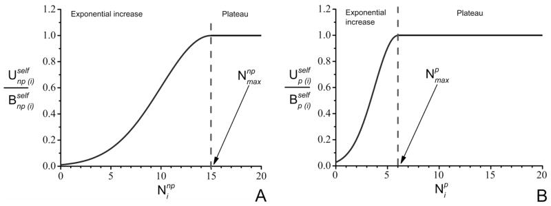
The dependence of the self energy contributions $U_{\mathit{self}}^{np}$ (A) and $U_{\mathit{self}}^p$ (B) of residue (i) on $N_i^{np}$ and $N_i^p$. Until the number of neighbors (polar or non-polar) reaches N_max, the self energy contributions increase exponentially. When number of neighbors is larger than N_max, the self energy contributions remain constant, taking the highest value B^self.

In cases of membrane proteins we represent the membrane by a grid of unified atoms, as we have done in our previous studies (e.g. see ref^19,31,34 ). This grid is used in a similar way to that used in Equation 9 and 10. The resulting self energy term which also reflects the boundaries between the protein and the membrane is given by:

$${\left[U_{\mathit{mem}}^{\mathit{self}}\left(N_{\mathit{mem}}^i\right)\right]}_{\mathit{burried}}=\{\begin{array}{ll}{U}_{\mathit{mem}}^{\mathit{self},0}exp\left[-{\left(\frac{R^{\mathit{solvent}}-W_{\mathit{mem}}/2}{L_s}\right)}^2\right],\hfill & R^{\mathit{solvent}}\le \frac{W_{\mathit{mem}}}{2}\hfill \\ U_{\mathit{mem}}^{\mathit{self},0},\hfill & R^{\mathit{solvent}}>\frac{W_{\mathit{mem}}}{2}\hfill \end{array}$$ (13)

where the term $U_{\mathit{mem}}^{\mathit{self},0}$ is given by :

$$U_{\mathit{mem}}^{\mathit{self},0}\left(N_{\mathit{mem}}^i\right)=\{\begin{array}{ll}{B}_{\mathit{mem}(i)}^{\mathit{self}}exp\left[-{\alpha }_U^{\mathit{mem}}{(N_{\mathit{mem}}^i-N_{\mathit{mem}}^{max})}^2\right],\hfill & 0<N_{\mathit{mem}}^i<N_{\mathit{mem}}^{max}\hfill \\ B_{\mathit{mem}(i)}^{\mathit{self}},\hfill & N_{\mathit{mem}}^i\ge N_{\mathit{mem}}^{max}\hfill \end{array}$$ (14)

The parameter R^solvent in Equation 13 is the distance to the closest solvent molecule, which is determined by a water grid around the system, and using the distance to the closest water grid point. W_mem is the width of the membrane atoms grid. L_s is a parameter that determines the effect of the burial of residue (i), and its suggested value (see^18,33,34) is one quarter of the membrane grid width W_mem. For a membrane grid spacing D_spacing = 2Å and width W_mem = 36Å, the value of L_s is taken as 9Ǻ (see ref^18,33,34 for more details). A description of the process of finding the contribution to the self energy of a fully buried ionizable residue from membrane grid atoms is depicted in Figure 3.

Figure 3.

A representation of an ionizable residue, surrounded by membrane grid points. Water grid atoms are also created, outside the membrane grid, and distances of water grid atoms from the residues side chain are calculated. The distance of the water grid atom closest to the ionizable residue is R^solvent. Also, W_mem is the total width of the membrane grid atoms with membrane spacing D_spacing. Half of this width, along with R^solvent is used in equation 13 to calculate ${\left[U_{\mathit{mem}}^{\mathit{self}}\left(N_{\mathit{mem}}^i\right)\right]}_{\mathit{burried}}$.

The effect of zwitterionic membrane head groups is simulated by placing positive and negative charges on the outer and the subsequent layer of the membrane grid, respectively. The corresponding electrostatic interactions with the protein charges were treated with Equation 7 and ε_eff = 20, which has been justified by earlier studies of the field from membrane head groups.

The third term in equation 2, $\mathrm{\Delta }{G}_{\mathit{side}}^{\mathit{polar}}$, is treated with equations identical to the ones used to calculate the self energies of the ionizable residues and is given by :

$$\mathrm{\Delta }{G}_{\mathit{side}}^{\mathit{polar}}=\sum _i\left[U_{\mathit{polar}}^{np}\left(N_i^{np}\right)+U_{\mathit{polar}}^p\left(N_i^p\right)+U_{\mathit{polar}}^{\mathit{mem}}\left(N_i^{\mathit{mem}}\right)\right]$$ (15)

where i runs over all polar residues (SER, THR, TYR, CYS, ASN, GLN), $N_i^{np},N_i^p$ and $N_i^{\mathit{mem}}$ are the number of non-polar residues, polar residues, and membrane atoms in the neighborhood of the i^th residue. The terms in Equation 15 are calculated by using equation 11 and 12, with exactly the same parameters given in Tables II and III. The functions $U_{\mathit{polar}}^{np},U_{\mathit{polar}}^p$ and $U_{\mathit{polar}}^{\mathit{mem}}$ are given by the same expression as in equations 9–10 and the corresponding parameter $B_p^{\mathit{pol}},B_{np}^{\mathit{pol}}$ and $B_{\mathit{mem}}^{\mathit{pol}}$ for each polar residue are given in Table V.

Table III.

The parameters for calculations of the free energy contributions to U for all types of residues (ionizable, polar and non polar/hydrophobic).

Parameter	Value
${\alpha }_U^p$	0.1
$N_{max}^p$	6
${\alpha }_U^{np}$	0.02
$N_{max}^{np}$	15
${\alpha }_U^{\mathit{mem}}$	0.05
$N_{max}^{\mathit{mem}}$	28
$R_{\mathit{cutoff}}^{\mathit{solvent}}$	18 Ǻ

Table V.

The parameters for the polar terms $(U_{\mathit{polar}}^p(N_i^p),U_{\mathit{polar}}^{np}(N_i^{np})$ and $U_{\mathit{polar}}^{\mathit{mem}}(N_i^{\mathit{mem}})$.

Residue	$B_p^{\mathit{pol}}$	$B_{np}^{\mathit{pol}}$	$B_{\mathit{mem}}^{\mathit{pol}}$
SER	−0.040	0.040	0.040
THR	−0.065	0.065	0.065
TYR	−0.125	0.125	0.125
CYS	−0.005	0.005	0.005
ASN	−0.215	0.215	0.215
GLN	−0.195	0.195	0.195

The last term in equation 2, $\mathrm{\Delta }{G}_{\mathit{side}}^{\mathit{hyd}}$, is treated by adopting similar model used in the self energy and polar free energy calculations, as follows.

$$\mathrm{\Delta }{G}_{\mathit{side}}^{\mathit{hyd}}=\sum _i\left[U_{\mathit{hyd}}^{np}\left(N_i^{\mathit{Ring}}\right)+U_{\mathit{hyd}}^p\left(N_i^p\right)+U_{\mathit{hyd}}^{\mathit{mem}}\left(N_i^{\mathit{mem}}\right)\right]$$ (16)

where i runs over all non-polar residues (ALA, LEU, ILE, VAL, PRO, MET, PHE, TRP), $N_i^p$ and $N_i^{\mathit{mem}}$ are the number of polar residues and membrane atoms in the neighborhood of the i^th non polar (hydrophobic) residue. They are calculated by using equation 11 and 12, with exactly the same parameters given in Table II. The functions $U_{\mathit{hyd}}^p$ and $U_{\mathit{hyd}}^{\mathit{mem}}$ are given by the same expression as in equations 10 and 13–14. The corresponding parameters are given in Table VI.

Table VI.

The parameters for the nonpolar and hydrophobic terms $U_{\mathit{hydro}}^p(N_i^p)$ and $U_{\mathit{hydro}}^{\mathit{mem}}(N_i^p)$.

Residue	$B_{\mathit{hydro}}^p$	$B_{\mathit{hydro}}^{\mathit{mem}}$
ALA	0.56	−1,07
LEU	0.80	−1.28
ILE	0.76	−1.61
VAL	0.80	−1.14
PRO	0.4	−1.71
MET	0.44	−0.71
PHE	1.0	−2.43
TRP	1.16	−3.21

The term $U_{\mathit{hyd}}^{np}$ however, is being treated in a different way, compared to its counterparts. That is, $U_{\mathit{hyd}}^{np}$ is given by:

$$U_{\mathit{hyd}}^{np}\left(N_i^{\mathit{Ring}}\right)=B_{\mathit{hyd}(i)}^{np}exp\left[-1.4(N_i^{\mathit{Ring}}/N_i^{\mathit{Water}})\right]$$ (17)

where $B_{\mathit{hyd}(i)}^{np}$ is a constant, similar in nature with the constants described in equations 8 to 14. $N_i^{\mathit{Ring}}$ is the number of implicit water grid points within a certain radius from the side chain center. $N_i^{\mathit{Water}}$ is the total number of implicit water grid points that this specific residue is surrounded with, when it is by itself in a water environment.

To calculate $N_i^{\mathit{Ring}}$ for each non polar residue (i), we create an implicit water grid around that residue and eliminate the grid points which collide with protein main chain atoms. Next we retain the grid points that are within the volume between the spheres of radii r_{hydro (i)} and r_{hydro (i)} + 4Ǻ from the center of the side chain atom of i^th residue. The rest of the grid points are eliminated. The total number of these grid points, is taken as the value of $N_i^{\mathit{Ring}}$. Figure 4 demonstrates how $N_i^{\mathit{Ring}}$ is calculated from the implicit water grid points, and the values of $B_{\mathit{hyd}(i)}^{np}$ and $N_i^{\mathit{Water}}$ are given in Table VII.

Figure 4.

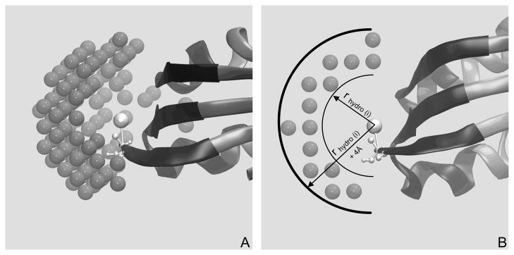
(A) Implicit water grid points, surrounding a CG residue of a protein (demonstrated in (B) The same water grid shown on (A) from a different viewing angle, which shows that the water grid points are only within a hollow spherical volume, created by two spheres of radius r_{hydro (i)} and r_{hydro (i)} + 4Ǻ.

Table VII.

The parameters for the hydrophobic (non polar) term $U_{\mathit{hyd}}^{np}\left(N_i^{\mathit{Ring}}\right)$

Residue	$B_{\mathit{hydro}}^{np}$	rhydro(Ǻ)	$N_i^{\mathit{Water}}$
ALA	−1,07	3.0	60
VAL	−1.28	4.5	110
LEU	−1.61	5.5	115
ILE	−1.14	6.0	120
PRO	−1.71	3.5	50
PHE	−0.71	5.0	130
TRP	−2.43	6.0	140
MET	−3.21	6.0	110

The free energy term ΔG_main

The main chain free energy ΔG_main is given by:

$$\mathrm{\Delta }{G}_{\mathit{main}}=\mathrm{\Delta }{G}_{\mathit{bond}}+\mathrm{\Delta }{G}_{\mathit{angle}}+\mathrm{\Delta }{G}_{\mathit{tor}}+\mathrm{\Delta }{G}_{i\mathit{tor}}+\mathrm{\Delta }{G}_{\mathit{tor}}^{\phi -\psi }+\mathrm{\Delta }{G}_{\mathit{main}}^{\mathit{Solv}}+\mathrm{\Delta }{G}_{HB}^{\mathit{TOTAL}}+\mathrm{\Delta }{G}_{\mathit{main}}^{qq}$$ (18)

where ΔG_bond, ΔG_angle, ΔG_tor, and ΔG_itor are contributions from the regular ENZYMIX force field. Also, the last term of the RHS of equation 18, $\mathrm{\Delta }{G}_{\mathit{main}}^{qq}$, is the charge-charge interaction free energy between the main chain atoms, which is calculated by equation 7 with a dielectric constant ε_eff = 10. The additional terms will be discussed below.

Since the secondary structure of proteins depends strongly on the solvation of the main chains we added the correction potential $\mathrm{\Delta }{G}_{\mathit{tor}}^{\phi -\psi }$ that is used to modify the gas phase potential. This solvation potential is given by

$$\mathrm{\Delta }{G}_{\mathit{tor}}^{\phi -\psi }=\sum _{i=1}^4{A}_{i}g\left(\phi -{\phi }_0^i,{\omega }_0^i\right)g\left(\psi -{\psi }_0^i,{\omega }_0^i\right)$$ (19)

where:

$$g(x,\omega )=exp\left(-0.693(1-cos(x))/sin(\omega /2)\right)$$ (20)

The values of ${\phi }_0^i$ and ${\psi }_0^i$ are chosen to represent the minima of the α-helix and β-sheet regions of the Ramachandran plot, while A_i and ${\omega }_0^i$ have been selected to tune the simple model α-helix and β-sheet regions to match those of the explicit model. The specific values of these parameters are listed in Table VIII.

Table VIII.

The parameters for the $\mathrm{\Delta }{\mathrm{G}}_{\text{tor}}^{\phi -\psi }$ term^a.

Region	Ai (kcal mol−1)	${\phi }_0^{\mathrm{i}}$	${\omega }_{\phi ,0}^{\mathrm{i}}$	${\psi }_0^{\mathrm{i}}$	${\omega }_{\psi ,0}^{\mathrm{i}}$
α - helix	−1	−95	8	−5	16
β - sheet	−10	−150	10	175	16
γ′ -turn	−3	−80	6	65	5
L-α - helix	−5	60	5	40	16

^aAngles in degrees and energies in kcal/mol.

The main chain solvation term is given by

$$\mathrm{\Delta }{G}_{\mathit{main}}^{\mathit{Solv}}=-B_{\mathit{solv}}\sum _i{U}_{\alpha ,i}$$ (21)

$$U_{\alpha ,i}=\{\begin{array}{ll}exp\left(-{\alpha }_{\theta }{\left(\mid {\theta }_i\mid -{\theta }_{max}\right)}^2\right),\hfill & \mid {\theta }_i\mid <{\theta }_{max}\hfill \\ 1,\hfill & \mid {\theta }_i\mid \ge {\theta }_{max}\hfill \end{array}$$ (22)

where B_solv = −2 and (i) runs over all residues in the sequence. The function θ, which reflects the percentage of polar residues around the C_α atom of a given residue (i), is given by

$${\theta }_i=\frac{N_{np,i}+N_{\mathit{mem},i}\left(N_p^{\theta \mathit{max}}/N_{\mathit{mem}}^{\theta \mathit{max}}\right)-N_p^{\theta \mathit{max}}}{N_p^{\theta \mathit{max}}}$$ (23)

where $N_p^{\theta \mathit{max}}$ is the maximum number of polar residues around a C_α atom (taken as 27 based on the total number of neighbors around the residue buried inside SecY translocon that was used as a test system); $N_{\mathit{mem}}^{\theta \mathit{max}}$ is the maximum number for membrane atoms around a C_α atom (taken as 33, based on using ALA in a membrane with membrane spacing of 4Ǻ as described in Figure 3). N_mem,i is the number of nonpolar and membrane residues around residue (i), which are calculated by the same approach used in the self energy calculation. The only difference is that we count the residues around the C_α and not the C_β atom, as done for the calculation of the self energy contributions.

The hydrogen bond function, $\mathrm{\Delta }{G}_{HB}^{\mathit{total}}$, is given by

$$\mathrm{\Delta }{G}_{HB}^{\mathit{total}}=\mathrm{\Delta }{G}_{HB}^{\mathit{water}}·U_{\alpha }^i·U_{\alpha }^j+\mathrm{\Delta }{G}_{HB}^{\mathit{mem}}·\left(1-U_{\alpha }^i·U_{\alpha }^j\right)$$ (24)

where we have

$$\mathrm{\Delta }{G}_{HB}^{\mathit{water}}=A_{\mathit{water}}·\left(\mathrm{\Delta }{G}_{HB}^{CG,0}+\mathrm{\Delta }{G}_{HB}^{\mathit{regular}}\right)+exp\left(-{\mu }_{HB}{\left(r_{ij}-r_{HB}\right)}^2\right)$$ (25)

and

$$\mathrm{\Delta }{G}_{HB}^{\mathit{mem}}=A_{\mathit{mem}}·\left(\mathrm{\Delta }{G}_{HB}^{CG,0}+\mathrm{\Delta }{G}_{HB}^{\mathit{regular}}\right)$$ (26)

where we use μ_HB = 22.2 Å⁻², r_HB =2.9Ǻ, A_water = 0.044 and A_MEM = 0.22. $\mathrm{\Delta }{\mathrm{G}}_{\text{HB}}^{\text{regular}}$ is the regular HB function used in the standard MOLARIS force field. $\mathrm{\Delta }{\mathrm{G}}_{\text{HB}}^{\text{CG},0}$ is given by

$$\mathrm{\Delta }{G}_{HB}^{CG,0}\{\begin{array}{ll}-1\hfill & r_{ij}\le r_0\hfill \\ -exp\left(-\mu {\left\{r_{ij}-r_0\right\}}^2\right)\hfill & r_{ij}>r_0\hfill \end{array}$$ (27)

with μ = 15, and r₀ = 2.0Ǻ. The scaling factors A_water and A_mem are given by the function

$$A=\left(1-0.8U_{\mathrm{\alpha }}^i{U}_{\mathrm{\alpha }}^j\right)/4.5$$ (28)

where in water, U_α is equal to 1 for all residues, and in this case we have

$$A_{\mathit{water}}\approx (1-0.8·1)/4.5=0.2/4.5=0.044$$ (29)

On the other hand in the membrane, U_α is equal to 0 for all residues, and from equation 24, we have

$$A_{\mathit{mem}}\approx (1-0.8·0)/4.5=1/4.5=0.22$$ (30)

The free energy term ΔG_main–side

ΔG_main–side consists of two parts, the electrostatic and the van der Waals parts:

$$\mathrm{\Delta }{G}_{\mathit{main}-\mathit{side}}=\mathrm{\Delta }{G}_{\mathit{main}-\mathit{side}}^{\mathit{elec}}+\mathrm{\Delta }{G}_{\mathit{main}-\mathit{side}}^{\mathit{VDW}}$$ (31)

The electrostatic part, $\mathrm{\Delta }{G}_{\mathit{main}-\mathit{side}}^{\mathit{elec}}$ is treated with the same electrostatic interactions as in equation 7, but with the ε_eff = 10.

The van der Waals for main-side interactions, $\mathrm{\Delta }{G}_{\mathit{main}-\mathit{side}}^{\mathit{VDW}}$ consists of two parts, a) the one where the side chain is a regular protein side chain, $\mathrm{\Delta }{G}_{\mathit{main}-\mathit{side}\mathit{protein}}^{\mathit{VDW}}$ and b) the one where the side chain is a membrane grid atom, $\mathrm{\Delta }{G}_{\mathit{main}-\mathit{side}\mathit{mem}}^{\mathit{VDW}}$. $\mathrm{\Delta }{G}_{\mathit{main}-\mathit{side}\mathit{protein}}^{\mathit{VDW}}$ is treated as a regular 12–6 potential, only that side chain is treated as a Carbon atom. Again, the van der Waals interactions of membrane grid atoms $\mathrm{\Delta }{G}_{\mathit{main}-\mathit{side}\mathit{mem}}^{\mathit{VDW}}$ are handled with the same treatment and the same equation, as discussed before for the calculation of the $\mathrm{\Delta }{G}_{\mathit{side}-\mathit{mem}}^{\mathit{vdw}}$. That is, we use:

$$\mathrm{\Delta }{G}_{\mathit{main}-\mathit{side}\mathit{mem}}^{\mathit{VDW}}=\sum _{i<j}\left[\frac{A_{ij}}{{(\overline{\alpha }+{r_{ij}}^6)}^2}-\frac{B_{ij}}{\overline{\alpha }+{r_{ij}}^6}\right]$$ (32)

$$\begin{array}{l}{A}_{ij}=A_i{A}_j\\ B_{ij}=B_i{B}_j\end{array}$$ (33)

where A_i, A_j and B_i, B_j are the vdw parameters for main chain atoms i and membrane grid atoms j. The parameter ᾱ for this case is taken as 2871.33 Å⁶.

Results and discussions

Key applications and validations

Our CG model has been used effectively in key applications and we will consider below some of the recent directions. In doing so, we will consider both validation studies and general structure function correlations.

Modeling Protein Stability and Folding Energy

Our previous approach for evaluation the absolute stability of proteins has been based on using the PDLD/S-LRA electrostatic model with focused dielectric constants (ref³²) where we searched for the optimal set of the effective dielectric ε_eff and the self energy PDLD dielectric ε_p. While the results obtained have been very encouraging (Figure 5), we attempted to obtain similar results with the more qualitative CG model. In the case of our CG model we replaced the more rigorous self energy calculations with the more implicit ΔG_self term. At any rate we refined the CG model by requiring the best fit to the observed absolute stability of a bench mark of proteins, expressing $\mathrm{\Delta }{G}_{\mathit{fold}}^{CG}$ as:

$$\mathrm{\Delta }{G}_{\mathit{fold}}^{CG}=\mathrm{\Delta }{G}_{\mathit{elec}}^{\mathit{fold}}+\mathrm{\Delta }{G}_{\mathit{side}}^{\mathit{polar}}+\mathrm{\Delta }{G}_{\mathit{side}}^{\mathit{hyd}}+c_1\mathrm{\Delta }{G}_{\mathit{side}-\mathit{side}}^{\mathit{vdw}}+c_2\mathrm{\Delta }{G}_{\mathit{solv}}^{CG}+c_3\mathrm{\Delta }{G}_{HB}^{\mathit{TOTAL}}$$ (34)

where the scaling constants c₁, c₂ and c₃ have the values of 0.1, 0.25 and 0.15 respectively. $\mathrm{\Delta }{G}_{\mathit{elec}}^{\mathit{fold}}$ is expressed by modifying Equation 6, using:

$$\mathrm{\Delta }{G}_{\mathit{elec}}^{\mathit{fold}}=-2.3RT\sum _i{Q}_i^{MC}·({pK}_a^i-{pK}_a^w)+\mathrm{\Delta }{G}_{QQ}+\mathrm{\Delta }{G}_Q^{\mathit{dev}}$$ (35)

where ΔG_QQ is the charge-charge interactions of all protein’s ionizable residues, and it is calculated by using Equation 7 with a distant dependent dielectric constant ε_eff(ij) of the form:

$${\epsilon }_{\mathit{eff}(ij)}=1+80\left(1+exp(-0.5r_{ij})\right)$$ (36)

where r_ij is the distance between the indicated ionizable residues, $\mathrm{\Delta }{G}_Q^{\mathit{dev}}$ is a correction term, which is given by:

$$\mathrm{\Delta }{G}_Q^{\mathit{dev}}=2.3RT\sum _i\left[(Q_{uf(i)}-\langle Q_i\rangle )·({pK}_a^w-pH)·(1-exp\left(-\mu ·\mid {pK}_a^i-{pK}_a^w\mid \right)\right]$$ (37)

Figure 5.

Absolute folding energies (stabilities) of various proteins, obtained using the PDLD/S LRA model (taken from ref³²). (A) The best fitted predictions, where low values of dielectric constants have been used for the buried ionizable residues. For the remaining residues, values of the dielectric constants ${\epsilon }_p^{\prime }$ and ${\epsilon }_{\mathit{eff}}^{\prime }$ are between 35 and 40. (B) The actual predictions of the absolute stabilities of the tested proteins, where individual predictions for specific dielectric constants ${\epsilon }_p^{\prime }$ and ${\epsilon }_{\mathit{eff}}^{\prime }$ have been averaged. For more information see ref³².

Here, 〈Q_i〉 is the MC averaged charge of the i^th residue, Q_{uf (i)} is the charge of residue (i) in water, and μ = 0.1. Q_i is the charge of each ionizable residue (i), which minimizes the electrostatic free energy. ${pK}_a^i$ and ${pK}_a^w$ are the intrinsic pK_a of the i^th ionizable residue, in protein and in water, respectively.

The results obtained after refining the CG model are given in Figure 6 and the corresponding results are summarized in Table IX. As seen from Figure 6, the CG model does not achieve the accuracy of the more explicit PDLD/S –LRA model in reproducing absolute folding energy. However the overall trend in stability is reproduced. It is important to realize that the fitting procedure reflects a compromise between different requirements. For example, we found out that we cannot get a quantitative agreement between the calculated and observed effects of hydrophobic mutations without getting serious deterioration in the agreement between the calculated and observed absolute stability. Apparently, as is the case with other models, it is hard to reproduce absolute folding energies quantitatively, but we believe that reproducing the observed trend is a very effective way of calibrating a CG model. We also note that we have the option of using the CG as a reference potential for moving into the explicit potential.¹⁹ This approach should be particularly effective in reproducing mutational effects on protein stability.¹⁹ It should also be pointed out that the CG should perform the best in exploring the electrostatic effect on protein stability. Considering the fact that the CG model allows for a very fast screening of protein stability, we also like to point out the our CG estimate can be evaluated for any protein by using the MOLARIS-XG³⁵ package.

Figure 6.

Absolute folding energies (stabilities) of various proteins (taken from ref³²), obtained using the CG model. The charges for each protein are calculated by using Monte Carlo minimization method, and the contributions to the folding free energy ΔG_fold have been described in equations 34 and 35.

Table IX.

Predicted and observed absolute stabilities of a set of proteins, using CG Model

Protein set	ΔGobs	ΔGcalc
Staphylococcal Nuclease	6.2	6.7
Staphylococcal Nuclease Δ+PHS75	11.9	7.5
Ribonuclease	10.5	10.7
Barstar	5.7	3.1
Bc CSP	5	8.7
SS07d	8	10.0
Chey	9.5	13.4
FeCyt b562	10.1	10.3
Thioredoxin	9	12.0
Apoflavodoxin	4.3	2.5
Barnase wt	8.8	11.2
Bnase W94F76	8	11.0
Bnase W94L76	7.5	10.2
Ec DHFR WT	6.1	8.5
Ec DHFR W22L77	6.2	6.7
Ec DHFR_W30A78	4.0	7.6
bCSP WT79	3.5	0.1
bCSP F27A79	2.7	−0.5
bCSP F17A79	2	−0.5
bCSP F15A79	1.2	−0.3
Ribosomal s6	8	6.0
λ-Repressor	4.6	7.7
Bs Hpr Phosphotransferase	4	3.7
Arc Repressor	4.6	7.7
GDH Domain2	4.9	12.7
Ferridoxina	-	-
Sac7d	7.4	12.4
Ubiquitin F45W	7.4	4.7
Interleucine	9.1	15.2
R_Nase A80	9.3	9.2
R_Nase T180	7.7	11.9

Observed values of protein stabilities have been found from ref³², unless otherwise stated.

^aFerridoxin without the SF₄ ligand is considered unstable.

Modeling Membrane Proteins

Some of the challenging applications of CG models involve the functions of membrane proteins. This include such problems as the insertion of proteins in membranes^29,36, the energetics of voltage activated proteins^37,38, the action of proton pumps^17,39 and transporters^40,41. While other CG models of membranes emphasize the properties of the membrane¹⁴ we follow our very early philosophy of using membrane grid (with induced dipoles) in studies of electrostatic effect in proteins and related systems^42,43, focusing on the electrostatic aspects of the model. This included calibration with respect to the insertion of charges in membranes and the insertion of peptides in membranes. The resulting model is described in the “Methods” section, and a validation of the model with respect to its performance in studies of charge insertion to a membrane is summarized in Figure 7. The calibration of the model is not completely unique due to the serious absence of relevant experimental studies and fully believable microscopic studies (see discussion in⁴⁴). Thus the current consensus energetics (which is open to modifications) is summarized in Table X. The insertion values obtained by our model are similar to those obtained by other CG approaches^45,46 and obviously with the emergence of more reliable experimental or microscopic results it will be easier to further refine the model. The recent applications include studies of the energetics of protein insertion into membranes through the translocon⁴⁴ (see Figure 8), the energetics of proton transport through the protein membrane interface in F₀-ATPase35 and the interplay between the translocon and the stalled ribosome⁴⁷. We believe that the main advances in our CG simulations of membrane proteins are based on the emphasis on the electrostatic aspects of the protein membrane system.

Figure 7.

The PMF profiles for the insertion of ARG into the membrane. The figure compares the free energy profiles for our CG model (dash line), microscopic calculations⁷³ (thick line) and a CG model⁷⁴ (thin line). This figure is taken from ref ³⁴.

Table X.

Examination and calibration of the energies of helix insertion into membranes.

Model	ΔGelec	ΔGhyd	ΔGsolv	ΔGHB	ΔGtot	Δ ΔGtot (wat→mem)	ΔΔGest (wat→mem)
polyA_wat	0.00	−4.44	−12.65	−5.12	−22.21
polyA_mem	0.00	−16.36	−0.49	−9.90	−26.75	−4.55	−(4÷5)
M2δ_wat	−0.74	−4.96	−19.24	−0.23	−25.17
M2δ_mem	0.16	−26.13	−6.25	−2.17	−34.40	−9.22	−(6.0÷11.3)
polyL_wat	0.00	−5.24	−8.52	−2.15	−15.91
polyL_mem	0.00	−34.72	−0.39	−5.11	−40.23	−24.32	−3.0
RR_wat	0.45	−11.99	−19.82	−3.91	−35.27
RR_mem	1.18	−54.82	−7.47	−7.88	−68.99	−33.72	—

Energies in kcal/mol. ΔG_tot, ΔG_elec, ΔG_hyd, ΔG_solv and ΔG_HB are, respectively, the total free energy (relative to water state), the electrostatic energy, the hydrophobic contribution, the main chain solvation and the hydrogen bond contribution. Δ ΔG_tot(wat→mem) is the free energy change for moving the peptide from water to membrane. Δ ΔG_est(wat→mem) designated estimated values of the free energy change, which includes: the observed value for the 20mer polyA^67,68, the value for the 23-amino-acid M2δ segment of the nicotinic acetylcholine receptor, estimated by other CG calculations^46,81, the value for the 12mer polyL estimated from microscopic simulations⁷³. Table is taken from ref⁴⁴.

Figure 8.

The CG free energy profiles for insertion into the TR (blue lines), into the membrane (red lines) and translocation (green lines) for the RR SP in the N_in (solid line) and N_out (dashed line) orientations. All profiles are plotted relative to the free energy of the N_in SP in water (at the very negative X). The data points were obtained from the calculations for the SP without the tail. Note that the difference between the energy of C_(in) and C_(out) is an artifact due to the fluctuations in the distance between the SP and the TR as well as due to the limited membrane spacing. The energy in the membrane is most probably too negative and indicated by the tentative gray lines. This figure is taken from ref ⁴⁴. (Please see the online version for the color figure).

Ionic solutions, ionic strength and external potentials

Another major challenge for simulations is the modeling of voltage activated proteins and to capture the microscopic physics of the interaction between the external potential and the protein charge. Although there have been significant advances in computational modeling efforts of ion channel energetics^27,48–53, the understanding of the voltage activation process is still rather limited. Not only that the exact structural changes during the activation process have not been fully determined, but also the energetics of the conformational transition and the coupling to the external voltage are far from being understood. Obtaining such a description requires one to capture the effect of the electrolytes between the protein/membrane system and the electrodes. Such a description is provided by our recent model^18,33 that represents the ionic solution as a grid whose spacing is taken here as Δ with a (volume element τ = Δ³) and placed at the center of the i^th grid point of residual charge ( $q_i^g$) determined by:

$$q_i^g=q_i^{+}+q_i^{-}$$ (38)

where

$$q_i^{\pm }=\frac{{\alpha }^{\pm }\left(N_{\mathit{box}}^{\pm }+N_{\mathit{bulk}}^{\pm }\right)e^{\mp \beta {\varphi }_i}}{\left({\displaystyle \sum _{i\in \mathit{box}}}{e}^{\mp \beta {\varphi }_i}+N_{\mathit{bulk}}^{\mathit{grid}}{e}^{\mp \beta {\varphi }_{\mathit{bulk}}}\right)}$$ (39)

where $q_i^{+}$ and $q_i^{-}$ are, respectively, the positive and negative fractional charges that are assigned to the i^th grid point, α^± is the ion charge of the electrolyte ions in atomic units (namely, ±1 for the 1:1 electrolyte used in our calculations), $N_{\mathit{box}}^{\pm }$ is the total number of cations/anions in the simulation box, $Q_{\mathit{box}}^{\pm }$ is the total charge of cations/anions in the simulation system given by $Q_{\mathit{box}}^{\pm }={\mathrm{\alpha }}^{\pm }{N}_{\mathit{box}}^{\pm }$, φ_i is the electrostatic potential (times a unit charge) at the i^th grid point and β = (k_BT)⁻¹. $N_{\mathit{bulk}}^{\mathit{grid}}$ is the number of grid points within the bulk system and ϕ_bulk is a constant potential on the bulk grid points. φ_i can be expressed as

$${\phi }_i=332\sum _j\frac{q_j^P}{{\mathrm{\epsilon }}_{\mathit{eff}}^{gp}{r}_{ij}}+332\sum _{k\ne i}\frac{q_k^g}{{\mathrm{\epsilon }}^{\mathit{wat}}{r}_{ik}}+V_i^{\mathit{ext}}$$ (40)

where $V_i^{\mathit{ext}}$ represents the external potential (times a unit charge ) on the i^th grid point that will be described below. Here, $q_j^P$ is the charge of the j^th protein residue (these charges are evaluated by MC procedure described above) and $q_k^g$ is the point charge at the k^th grid point (representing the excess net charge of the k^th volume element).

The final set of the grid charges (q^g) are obtained iteratively (see SI), and the effect of the ionic strength is evaluated as outlined in³³.

This model reproduces the standard test cases of the Debye-Huckel and Gouy-Chapman models, as well as the potential between electrodes (Figure 9, the potential between electrodes). However, in contrast to continuum models, our CG model represent explicitly the medium between the membrane an the electrode and allow one to obtain explicitly key quantities such as gating charges and gating current, using the change in charge on the ionic grid.^18,33 This allow one to move beyond treatments that look at the shifts of the protein charges assuming basically a linear model (e.g. ⁴⁹).

Figure 9.

(a) The electrolyte potential (in Volt) and (b) the electrolyte charge distribution along Z-axis for a system with two electrodes (external potential is 100 mV). The results for two different electrolyte concentrations are shown: 10 mM (red) and 100 mM (blue). The linear electrode potential (in absence of electrolyte) is shown as a reference in (a) (black). Calculations have been performed with (17 X 17) periodic images in the XY plane. This figure is taken from ref ³³. (Please see the online version for the color figure).

Another use of our ionic grid is in treating highly charged proteins (see below). The implementation of our CG grid model in studies of the effect of electrode potentials included the introduction of a specialized bulk region that allows us to extend the simulation system to very large dimensions and thus to explore the realistic effects of the electrodes. Furthermore, we also represent the electrodes in an explicit way using both explicit surface charges (with periodic boundary conditions) and the equivalent vacuum field. Here the insistence on explicit model of the electrolytes allow us to represent explicitly all the key elements of voltage activated channels and thus to overcome some of the key uncertainties in the field.

Unfolding and folding processes

The CG model can be used (at least in principle) to explore the nature of folding paths, the relevant activation barriers and the linear free energy relationships (LFER) observed in folding processes^10,54. This can be done both on an approximated level by the CG potential or by using the CG potential as a reference potential for the explicit potential.^19,22 While we have not yet moved in this interesting direction, we explored in a preliminary way the performance of the model in reproducing the energetics of the unfolding of the Ribosomal Protein S6 and its mutants as it was described in the work of Oliveberg and his coworkers⁵⁵. Three specific systems have been studied: 1) the WT protein at pH~7, whose charges include 16 basic and 16 acidic amino acid residues and the charges at the N and C terminals. 2) a highly charged mutant at pH~7, where all original basic residues of the WT have been mutated to SER, 16 acidic residues and the charges at the N and C terminals and finally, 3) the same mutant -all basic residues mutated to SER- but studied at a very low pH~2, forcing the acidic amino acids and the N terminal to be in a protonated state, thus being uncharged, leaving an almost uncharged mutant with only one positive charge at the N terminal.

The calculations of the absolute stability gave reasonable but not perfect results (see Table XI), after considering the effect of the ionic strength and the fact that we were forced to scale down the hydrophobic effect that seems to have a large effect in case 3. However the main challenge has been in exploring the unfolding barrier. This was done in a rather primitive way by unfolding the protein systems (all three studied) by moving in a direction that minimizes the so called contact order (CO). That is, the CO that provides an effective way to explore folding landscapes (see for example the review paper of Fersht⁵⁴ ) is given by

Table XI.

Predicted and observed absolute stabilities of the Ribosomal protein S6 and its mutants.

Systems	Observed ΔGfold	Calculated ΔGfold
Ribosomal S6 WT +17 −17	−8.2	−6.0
aRibosomal S6 +1 −17	−2.9	−3.1
aRibosomal S6 +1	−4.0	3.5

Energies in kcal/mol. Systems and observed absolute stabilities taken from ref⁵⁵.

^aIonic strength of 150 mM has been used to calculate absolute stabilities.

$$CO=\frac{1}{L·N}\sum _{}^N\mathrm{\Delta }{Z}_{ij}$$ (41)

where N is the total number of contacts in the protein, ΔZ_ij is the number of residues separating contacts i and j, and L is the total number of residues in the protein.

Here we look for a function that reduces the CO by applying an energy constraint of the form:

$$\begin{array}{l}{E}_{C_{\alpha }}=\sum _{\begin{array}{c}j>i\\ j-i\ge 4\end{array}}\frac{A}{r_{ij}}\left(N_{C_{\alpha }}-N_{un\mathit{fold}}\right){\theta }_{ij}\\ \begin{array}{ll}{\theta }_{ij}=1\hfill & r_{ij}\le R_{\mathit{cutoff}}^{C_{\alpha }}\hfill \\ {\theta }_{ij}=0\hfill & r_{ij}>R_{\mathit{cutoff}}^{C_{\alpha }}\hfill \end{array}\end{array}$$ (42)

Where r_ij is the distance between C_α atoms of the i^th and the j^th residues, N_unfold is a parameter that specifies the desired value of long ranged contacts during a simulation, $R_{\mathit{cutoff}}^{C_{\alpha }}$ is the C_α cut-off distance and N_Cα is the total number of contact pairs. Here we used N_unfold = 0.015 and A =10, whereas the value of $R_{\mathit{cutoff}}^{C_{\alpha }}$ was changed gradually between 6Å (fully folded) and 15Å (fully unfolded). The simulations with the constraint described in Equation 42 induce a gradual unfolding along the coordinate that minimizes N_Cα, forcing the CO to become smaller.

The results for the unfolding profile for the WT and the −17+1 proteins are given in Figure 10. The most interesting part is the enormous effect when including the ionic strength on the highly charged protein. In this respect the results are very encouraging. On the other hand the results for the + 1 protein are disappointing, not capturing the observed trend. Here the only encouraging part is the fact that the folding barrier (around 7 kcal/mol) is very small in agreement with the experimental observation⁵⁵.

Figure 10.

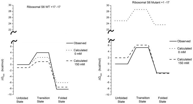
Barriers (observed and calculated) for the study of Ribosomal S6 WT and the highly charged mutant +1-17.

General Applications

The electrostatically based CG model has been found to be extremely useful in studies of structure-function relationships in large biological assemblies, where it is almost impossible to determine and analyze the origin of the functional coupling using traditional brute-force simulation approaches. Several cellular phenomena like the mechano-chemical coupling in the rotational motor F₁F₀-ATPsynthase^56,57, action of the voltage-gated ion-channels18 and unstalling of the nascent peptide in the ribosome-translocon assembly⁴⁷ have been studied to elucidate the underlying physical principles driving the functional directionality in such complexes. Here we will consider some of our recent advances.

The F₁F₀-ATPsynthase is a ubiquitous cellular engine composed of two rotational motors, the cytoplasmic F₁ coupled to the membrane embedded F₀ units. The F₀ rotor uses the energy of the proton transport across the cellular membrane to rotate the membrane embedded c-ring, while the F₁ couples the rotation of the c-ring with its central stalk (γ subunit) to generate ATP from ADP and P_i. In spite of numerous simulation and phenomenological studies^58,59, the nature of the coupling between chemical and mechanical events in the F₁F₀-ATPsynthase has remained elusive. In the case of F₁-ATPase, we succeeded to produce the vectorial nature of the γ subunit rotation coupled to the conformational changes of the α/β catalytic subunits. The CG electrostatic free energy surface revealed the presence of the 80º/40º stepwise rotation of the system that has been observed in several single molecule experiments⁶⁰, but is especially difficult to understand from the structural perspectives, owing to the large system size and very long time scales extending beyond the millisecond regime. The CG electrostatic free energy surface coupled to the ATP hydrolysis and product release free energies (Figure 11) could successfully predict the role of the high electrostatic barrier of the catalytic subunit conformational changes in funneling the chemical step after the 80º γ rotation. This produces the “catalytic dwell” between the 80º/40º steps as observed from the experiments⁵⁶.

Figure 11.

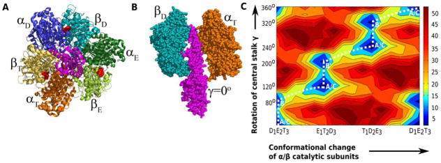
The structure of F₁-ATPase is shown from the (A) membrane side and (B) along the vertical direction parallel to the central γ stalk. The α catalytic subunits are shown in deep blue, deep green and orange, while β units are shown in cyan, light green and yellow. The γ stalk is shown in magenta. The nucleotide occupancies of the β subunits are depicted as T (ATP bound), D (ADP bound) or E (empty) states. (C) The CG electrostatic free energy surface of the rotation of γ coupled to the α/β conformational changes reflects stepwise 80°/40° features. This figure is taken from ref⁵⁶ (Please see the online version for the color figure).

Our CG model has also been successfully applied to the problem of understanding the electrochemically driven F₀ motor function. Phenomenological models have attempted to understand the action of the F₀ c-ring rotation coupled to the proton transfer from the low to high pH reservoirs across the membrane^61,62, but once again, a quantitative structure-function relationship elucidating the physical nature of the directional rotation has been missing. We utilized the CG model to generate the electrostatic free energy surface of the c-ring rotation coupled to the proton transport from the P side (pH=5) to the N side (pH=8) of the membrane. As revealed from the CG surface, the molecular origin of the directional c-ring rotation is mostly due to the asymmetry of the proton transport path on the N and P sides of the F₀, rather than driven by the energetics of the centrally placed salt bridge between the c-ring and the stator subunit-a⁵⁷. These studies also produce a clear conceptual basis (Figure 12) of the electrostatic driven energy transduction process in the F₁F₀ motor that could be further explored in the future.

Figure 12.

The structure of the membrane embedded F₀-ATPase is shown from the (A) XY plane of the membrane and (B) along the Z direction of the membrane (membrane width). The c-ring helices are shown in green while subunit-a is shown in orange. The centrally located ASP-ARG ion pair is shown in red/blue ball and stick representation. The proton positions along the cring/subunit-a interface are designated as N1 to N5 and P1 to P6 in the N and P sides of the membrane. The N and P sides of the membrane correspond to the physiological pH of 8 and 5 respectively. (C) The electrostatic free energy map of the proton transport coupled to the rotation of the c-ring reflects the asymmetry of the proton transport paths in the N and P sides of the central Arg. This figure is taken from ref⁵⁷ (Please see the online version for the color figure).

Another large biological system that was explored with our CG model is the translocon complex. It is responsible for protein translocation across the membrane as well as their proper integration into the membrane through the so called lateral gate.^29,36 In exploring this system we investigated several puzzling questions related to the translocon-assisted membrane protein integration. One of such questions involves the mechanism of membrane insertion of charged residues. The discrepancy between the experimental and theoretical studies led to multiple attempts to resolve the issue^63–66. To advance on this front we used our CG model to estimate the energetics of the transmembrane helix with central ionized arginine in the presence of the translocon and other helixes³⁴. Our study indicated that the free energy of inserting arginine from water to membrane could be substantially reduced by interaction with other helix. Another important question related to the translocon-assisted protein insertion is the mechanism of establishing proper membrane protein topology. It is known from experiments that some mutations of the translocon or flanking residues of the peptide transmembrane domain affect final protein orientation in the membrane^67,68. This subject is complicated by the fact that little is known about the mechanism of membrane integration as well as about the intermediate structures of the peptide during the insertion. Here we challenged ourselves to obtain the complete free energy profile for the protein translocation through the translocon as well as membrane integration. By applying several constraints on the system we were able to obtain the profile⁴⁴, which we used to investigate the effect of different mutations and the ribosome binding. Comparison with experimental data led to the conclusion that the insertion process is most likely a non-equilibrium process and the peptide topology is controlled by the barrier of inserting into the translocon. The obtained free energy profile allowed us to approach fundamental questions regarding the nature of the coupling between two large biological systems – translocon and ribosome. That is, we investigated the origin of the biphasic pulling force from the translocon that, as was shown experimentally⁶⁹, allows releasing the stalling of the elongated nascent peptide chain from the ribosome. Combining the estimate of the chemical barriers of the peptide bond formation for the regular and stalled peptide sequences with the profile for the translocon-assisted protein membrane integration and performing the Langevin dynamics simulations of the ribosome/translocon model, we were able to reproduce the experimental effect⁴⁷ (see Figure 13). This and other studies highlight the importance of obtaining the free energy profile for the thorough understanding of the mechanisms underlying different biological processes.

Figure 13.

The results of LD simulation of the peptide penetration process and the stalling effect. The figure describes the time dependence of x_istall and x₁ for a peptide chain with 40 and 36 units, which corresponds to L = 31 (blue) and 27 (red), respectively. [The barriers used for the LD simulations were obtained by scaling down the energy terms by 0.43. This allowed simulating the insertion process in a relatively short time and then estimating the relevant time for the actual barriers by using the corresponding Boltzmann probability.]. The snapshots on the top and bottom of the plot shows the configuration of the nascent peptide chain for L = 31 and L = 27, respectively. The ribosome and TR are shown schematically, the starting configuration of the nascent chain is in cyan, the leading particle (x₁) is in red, and all other particles added to the growing chain are shown in magenta. The interpolated time (that should be obtained without scaling) for L = 31 and L = 27 are 6 min and 36 min, respectively. Other parameters can lead to a larger time difference. This figure is taken from ref⁴⁷ (Please see the online version for the color figure).

Concluding Remarks

This work considers recent refinements and applications of our CG model. This model has been calibrated on absolute protein stabilities and other effects with emphasis on electrostatic effects that are arguably the most important factors in structure function correlation. The model has been found to provide a very powerful tool for exploring complex biological systems. This includes specialized applications like insertion of proteins through the translocon^34,44,47 or more general studies of conformational coupling in molecular motors^56,57, as well as the activation of voltage activated channels.^18,33

In considering the CG strategy, we realize that it is not a perfect strategy; however in many cases it gives the best option for capturing the function of complex biological systems. This is likely to be true for some time, despite the great increase in computer power, considering the enormous convergence problems especially since the key functional properties seem to be dictated by electrostatic effects.

Obviously after capturing the main physics behind the function of a given system it would be important to move to a more explicit description. Here it may be useful to exploit our ability to move from the CG to the corresponding explicit model.^19,22 This option, that has not been exploited sufficiently, can be considered as a version of our paradynamics strategy^1,22–24 were we can convert the qualitative CG findings to more quantitative conclusions. Of course, it is essential to obtain sufficient convergence, but the PD strategy allows one to obtain faster convergence than full exploration of the complete free energy surface by the explicit model.

Our CG studies indicate that the electrostatic contribution by far play the most crucial role on dictating the functional properties of biological systems. This confirms our many previous findings^31,70,71 as well as those of others,^36,72 that electrostatic energies provide the most effective way of correlating structure and functions. Thus, we anticipate that our CG model (which is implemented in the program MOLARIS-XG³⁵) offers one of the best current options of modeling protein function due to its focus on the electrostatic contributions.

References

- 1.Kamerlin SC, Vicatos S, Dryga A, Warshel A. Coarse-grained (multiscale) simulations in studies of biophysical and chemical systems. Ann Rev Phys Chem. 2011;62:41–64. doi: 10.1146/annurev-physchem-032210-103335. [DOI] [PubMed] [Google Scholar]
- 2.Levitt M, Warshel A. Computer Simulation of Protein Folding. Nature. 1975;253(5494):694–698. doi: 10.1038/253694a0. [DOI] [PubMed] [Google Scholar]
- 3.Warshel A, Levitt M. Folding and Stability of Helical Proteins - Carp Myogen. J Mol Biol. 1976;106(2):421–437. doi: 10.1016/0022-2836(76)90094-2. [DOI] [PubMed] [Google Scholar]
- 4.Taketomi H, Ueda Y, Go N. Studies on protein folding, unfolding and fluctuations by computer simulation. I. The effect of specific amino acid sequence represented by specific inter-unit interactions. International journal of peptide and protein research. 1975;7(6):445–459. [PubMed] [Google Scholar]
- 5.Nymeyer H, Garcia AE, Onuchic JN. Folding funnels and frustration in off-lattice minimalist protein landscapes. Proceedings of the National Academy of Sciences of the United States of America. 1998;95(11):5921–5928. doi: 10.1073/pnas.95.11.5921. [DOI] [PMC free article] [PubMed] [Google Scholar]
- 6.Dill KA. Dominant forces in protein folding. Biochemistry. 1990;29:7133–7155. doi: 10.1021/bi00483a001. [DOI] [PubMed] [Google Scholar]
- 7.Heath AP, Kavraki LE, Clementi C. From coarse-grain to all-atom: toward multiscale analysis of protein landscapes. Proteins. 2007;68(3):646–661. doi: 10.1002/prot.21371. [DOI] [PubMed] [Google Scholar]
- 8.Hinds DA, Levitt M. A lattice model for protein structure prediction at low resolution. Proceedings of the National Academy of Sciences of the United States of America. 1992;89(7):2536–2540. doi: 10.1073/pnas.89.7.2536. [DOI] [PMC free article] [PubMed] [Google Scholar]
- 9.Shakhnovich E, Abkevich V, Ptitsyn O. Conserved residues and the mechanism of protein folding. Nature. 1996;379:96–98. doi: 10.1038/379096a0. [DOI] [PubMed] [Google Scholar]
- 10.Wolynes PG. Recent successes of the energy landscape theory of protein folding and function. Quarterly reviews of biophysics. 2005;38(4):405–410. doi: 10.1017/S0033583505004075. [DOI] [PubMed] [Google Scholar]
- 11.Wu C, Shea JE. Coarse-grained models for protein aggregation. Curr Opin Struct Biol. 2011;21(2):209–220. doi: 10.1016/j.sbi.2011.02.002. [DOI] [PubMed] [Google Scholar]
- 12.Tozzini V. Coarse-grained models for proteins. Curr Opin Struct Biol. 2005;15(2):144–150. doi: 10.1016/j.sbi.2005.02.005. [DOI] [PubMed] [Google Scholar]
- 13.Guardiani C, Livi R, Cecconi F. Coarse Grained Modeling and Approaches to Protein Folding. Curr Bioinform. 2010;5(3):217–240. [Google Scholar]
- 14.Marrink SJ, Risselada HJ, Yefimov S, Tieleman DP, de Vries AH. The MARTINI force field: Coarse grained model for biomolecular simulations. Journal of Physical Chemistry B. 2007;111(27):7812–7824. doi: 10.1021/jp071097f. [DOI] [PubMed] [Google Scholar]
- 15.Voth GA. Multiscale Simulation of Multiprotein Assemblies: The Challenges of Ultra-Coarse-Graining. Biophys J. 2013;104(2):376a–376a. [Google Scholar]
- 16.Hyeon C, Thirumalai D. Capturing the essence of folding and functions of biomolecules using coarse-grained models. Nat Commun. 2011:2. doi: 10.1038/ncomms1481. [DOI] [PubMed] [Google Scholar]
- 17.Zhang B, Miller TF. Long-Timescale Dynamics and Regulation of Sec-Facilitated Protein Translocation. Cell Rep. 2012;2(4):927–937. doi: 10.1016/j.celrep.2012.08.039. [DOI] [PMC free article] [PubMed] [Google Scholar]
- 18.Dryga A, Chakrabarty S, Vicatos S, Warshel A. Realistic simulation of the activation of voltage-gated ion channels. Proceedings of the National Academy of Sciences of the United States of America. 2012;109(9):3335–3340. doi: 10.1073/pnas.1121094109. [DOI] [PMC free article] [PubMed] [Google Scholar]
- 19.Messer BM, Roca M, Chu ZT, Vicatos S, Kilshtain AV, Warshel A. Multiscale simulations of protein landscapes: Using coarse-grained models as reference potentials to full explicit models. Proteins: Struct Funct and Bioinf. 2010;78(5):1212–1227. doi: 10.1002/prot.22640. [DOI] [PMC free article] [PubMed] [Google Scholar]
- 20.Lifson S, Warshel A. Consistent Force Field for Calculations of Conformations Vibrational Spectra and Enthalpies of Cycloalkane and N-Alkane Molecules. J Chem Phys. 1968;49(11):5116. [Google Scholar]
- 21.Warshel A, Levitt M, Lifson S. Consistent Force Field for Calculation of Vibrational Spectra and Conformations of Some Amides and Lactam Rings. J Mol Spectrosc. 1970;33(1):84. [Google Scholar]
- 22.Fan ZZ, Hwang JK, Warshel A. Using simplified protein representation as a reference potential for all-atom calculations of folding free energy. Theor Chem Acc. 1999;103(1):77–80. [Google Scholar]
- 23.Plotnikov NV, Warshel A. Exploring, Refining, and Validating the Paradynamics QM/MM Sampling. Journal of Physical Chemistry B. 2012;116(34):10342–10356. doi: 10.1021/jp304678d. [DOI] [PubMed] [Google Scholar]
- 24.Plotnikov NV, Kamerlin SC, Warshel A. Paradynamics: An Effective and Reliable Model for Ab Initio QM/MM Free-Energy Calculations and Related Tasks. J Phys Chem B. 2011;115(24):7950–7962. doi: 10.1021/jp201217b. [DOI] [PMC free article] [PubMed] [Google Scholar]
- 25.Izvekov S, Voth GA. A multiscale coarse-graining method for biomolecular systems. Journal of Physical Chemistry B. 2005;109(7):2469–2473. doi: 10.1021/jp044629q. [DOI] [PubMed] [Google Scholar]
- 26.Warshel A, Lifson S. Consistent Force Field Calculations.2. Crystal Structures, Sublimation Energies, Molecular and Lattice Vibrations, Molecular Conformations, and Enthalpies of Alkanes. J Chem Phys. 1970;53(2):582. [Google Scholar]
- 27.Jensen MO, Jogini V, Borhani DW, Leffler AE, Dror RO, Shaw DE. Mechanism of Voltage Gating in Potassium Channels. Science. 2012;336(6078):229–233. doi: 10.1126/science.1216533. [DOI] [PubMed] [Google Scholar]
- 28.Voelz VA, Bowman GR, Beauchamp K, Pande VS. Molecular Simulation of ab Initio Protein Folding for a Millisecond Folder NTL9(1–39) J Am Chem Soc. 2010;132(5):1526. doi: 10.1021/ja9090353. [DOI] [PMC free article] [PubMed] [Google Scholar]
- 29.Kamerlin SCL, Haranczyk M, Warshel A. Progress in Ab Initio QM/MM Free-Energy Simulations of Electrostatic Energies in Proteins: Accelerated QM/MM Studies of pK(a), Redox Reactions and Solvation Free Energies. Journal of Physical Chemistry B. 2009;113(5):1253–1272. doi: 10.1021/jp8071712. [DOI] [PMC free article] [PubMed] [Google Scholar]
- 30.Roca M, Messer B, Warshel A. Electrostatic contributions to protein stability and folding energy. FEBS letters. 2007;581(10):2065–2071. doi: 10.1016/j.febslet.2007.04.025. [DOI] [PubMed] [Google Scholar]
- 31.Warshel A, Sharma PK, Kato M, Parson WW. Modeling electrostatic effects in proteins. Bba-Proteins Proteom. 2006;1764(11):1647–1676. doi: 10.1016/j.bbapap.2006.08.007. [DOI] [PubMed] [Google Scholar]
- 32.Vicatos S, Roca M, Warshel A. Effective approach for calculations of absolute stability of proteins using focused dielectric constants. Proteins-Structure Function and Bioinformatics. 2009;77(3):670–684. doi: 10.1002/prot.22481. [DOI] [PMC free article] [PubMed] [Google Scholar]
- 33.Dryga A, Chakrabarty S, Vicatos S, Warshel A. Coarse grained model for exploring voltage dependent ion channels. Biochim Biophys Acta. 2012;1818(2):303–317. doi: 10.1016/j.bbamem.2011.07.043. [DOI] [PMC free article] [PubMed] [Google Scholar]
- 34.Rychkova A, Vicatos S, Warshel A. On the energetics of translocon-assisted insertion of charged transmembrane helices into membranes. Proceedings of the National Academy of Sciences of the United States of America. 2010;107(41):17598–17603. doi: 10.1073/pnas.1012207107. [DOI] [PMC free article] [PubMed] [Google Scholar]
- 35.Warshel A, et al. Molaris-XG: Theoretical Background and Practical Examples. 2013 available at: http://laetro.usc.edu/programs/doc/theory_molaris_9.11.pdf.
- 36.Perutz MF. Electrostatic Effects in Proteins. Science. 1978;201(4362):1187–1191. doi: 10.1126/science.694508. [DOI] [PubMed] [Google Scholar]
- 37.Bezanilla F. How membrane proteins sense voltage. Nat Rev Mol Cell Bio. 2008;9(4):323–332. doi: 10.1038/nrm2376. [DOI] [PubMed] [Google Scholar]
- 38.Swartz KJ. Sensing voltage across lipid membranes. Nature. 2008;456(7224):891–897. doi: 10.1038/nature07620. [DOI] [PMC free article] [PubMed] [Google Scholar]
- 39.Zhang B, Arun G, Mao YS, Lazar Z, Hung GN, Bhattacharjee G, Xiao XK, Booth CJ, Wu J, Zhang CL, Spector DL. The lncRNA Malat1 Is Dispensable for Mouse Development but Its Transcription Plays a cis-Regulatory Role in the Adult. Cell Rep. 2012;2(1):111–123. doi: 10.1016/j.celrep.2012.06.003. [DOI] [PMC free article] [PubMed] [Google Scholar]
- 40.Forrest LR. (Pseudo-)Symmetrical Transport. Science. 2013;339(6118):399–401. doi: 10.1126/science.1228465. [DOI] [PubMed] [Google Scholar]
- 41.Rees DC, Johnson E, Lewinson O. ABC transporters: the power to change. Nat Rev Mol Cell Bio. 2009;10(3):218–227. doi: 10.1038/nrm2646. [DOI] [PMC free article] [PubMed] [Google Scholar]
- 42.Alden RG, Parson WW, Chu ZT, Warshel A. Calculations of Electrostatic Energies in Photosynthetic Reaction Centers. J Am Chem Soc. 1995;117(49):12284–12298. [Google Scholar]
- 43.Aqvist J, Warshel A. Energetics of Ion Permeation through Membrane Channels - Solvation of Na+ by Gramicidin-A. Biophys J. 1989;56(1):171–182. doi: 10.1016/S0006-3495(89)82662-1. [DOI] [PMC free article] [PubMed] [Google Scholar]
- 44.Rychkova A, Warshel A. Exploring the nature of the translocon-assisted protein insertion. Proceedings of the National Academy of Sciences of the United States of America. 2013;110(2):495–500. doi: 10.1073/pnas.1220361110. [DOI] [PMC free article] [PubMed] [Google Scholar]
- 45.Hall BA, Chetwynd AP, Sansom MSP. Exploring Peptide-Membrane Interactions with Coarse-Grained MD Simulations. Biophys J. 2011;100(8):1940–1948. doi: 10.1016/j.bpj.2011.02.041. [DOI] [PMC free article] [PubMed] [Google Scholar]
- 46.Kessel A, Haliloglu T, Ben-Tal N. Interactions of the M2 delta segment of the acetylcholine receptor with lipid bilayers: A continuum-solvent model study. Biophys J. 2003;85(6):3687–3695. doi: 10.1016/S0006-3495(03)74785-7. [DOI] [PMC free article] [PubMed] [Google Scholar]
- 47.Rychkova A, Mukherjee S, Bora RP, Warshel A. Simulating the pulling of stalled elongated peptide from the ribosome by the translocon. Proceedings of the National Academy of Sciences of the United States of America. 2013;110(25):10195–10200. doi: 10.1073/pnas.1307869110. [DOI] [PMC free article] [PubMed] [Google Scholar]
- 48.Khalili-Araghi F, Tajkhorshid E, Roux B, Schulten K. Molecular Dynamics Investigation of the omega-Current in the Kv1. 2 Voltage Sensor Domains. Biophys J. 2012;102(2):258–267. doi: 10.1016/j.bpj.2011.10.057. [DOI] [PMC free article] [PubMed] [Google Scholar]
- 49.Khalili-Araghi F, Jogini V, Yarov-Yarovoy V, Tajkhorshid E, Roux B, Schulten K. Calculation of the Gating Charge for the Kv1. 2 Voltage-Activated Potassium Channel. Biophys J. 2010;98(10):2189–2198. doi: 10.1016/j.bpj.2010.02.056. [DOI] [PMC free article] [PubMed] [Google Scholar]
- 50.Henrion U, Renhorn J, Borjesson SI, Nelson EM, Schwaiger CS, Bjelkmar P, Wallner B, Lindahl E, Elinder F. Tracking a complete voltage-sensor cycle with metal-ion bridges. Proceedings of the National Academy of Sciences of the United States of America. 2012;109(22):8552–8557. doi: 10.1073/pnas.1116938109. [DOI] [PMC free article] [PubMed] [Google Scholar]
- 51.Schwaiger CS, Bjelkmar P, Hess B, Lindahl E. 3(10)-Helix Conformation Facilitates the Transition of a Voltage Sensor S4 Segment toward the Down State. Biophys J. 2011;100(6):1446–1454. doi: 10.1016/j.bpj.2011.02.003. [DOI] [PMC free article] [PubMed] [Google Scholar]
- 52.Delemotte L, Tarek M, Klein ML, Amaral C, Treptow W. Intermediate states of the Kv1. 2 voltage sensor from atomistic molecular dynamics simulations. Proceedings of the National Academy of Sciences of the United States of America. 2011;108(15):6109–6114. doi: 10.1073/pnas.1102724108. [DOI] [PMC free article] [PubMed] [Google Scholar]
- 53.Freites JA, Schow EV, White SH, Tobias DJ. Microscopic Origin of Gating Current Fluctuations in a Potassium Channel Voltage Sensor. Biophys J. 2012;102(11):A44–A46. doi: 10.1016/j.bpj.2012.04.021. [DOI] [PMC free article] [PubMed] [Google Scholar]
- 54.Fersht AR. Transition-state structure as a unifying basis in protein-folding mechanisms: Contact order, chain topology, stability, and the extended nucleus mechanism. Proceedings of the National Academy of Sciences of the United States of America. 2000;97(4):1525–1529. doi: 10.1073/pnas.97.4.1525. [DOI] [PMC free article] [PubMed] [Google Scholar]
- 55.Kurnik M, Hedberg L, Danielsson J, Oliveberg M. Folding without charges. Proceedings of the National Academy of Sciences of the United States of America. 2012;109(15):5705–5710. doi: 10.1073/pnas.1118640109. [DOI] [PMC free article] [PubMed] [Google Scholar]
- 56.Mukherjee S, Warshel A. Electrostatic origin of the mechanochemical rotary mechanism and the catalytic dwell of F1-ATPase. Proceedings of the National Academy of Sciences of the United States of America. 2011;108(51):20550–20555. doi: 10.1073/pnas.1117024108. [DOI] [PMC free article] [PubMed] [Google Scholar]
- 57.Mukherjee S, Warshel A. Realistic simulations of the coupling between the protomotive force and the mechanical rotation of the F0-ATPase. Proceedings of the National Academy of Sciences of the United States of America. 2012;109(37):14876–14881. doi: 10.1073/pnas.1212841109. [DOI] [PMC free article] [PubMed] [Google Scholar]
- 58.Wang HY, Oster G. Energy transduction in the F-1 motor of ATP synthase. Nature. 1998;396(6708):279–282. doi: 10.1038/24409. [DOI] [PubMed] [Google Scholar]
- 59.Pu JZ, Karplus M. How subunit coupling produces the gamma-subunit rotary motion in F-1-ATPase. Proceedings of the National Academy of Sciences of the United States of America. 2008;105(4):1192–1197. doi: 10.1073/pnas.0708746105. [DOI] [PMC free article] [PubMed] [Google Scholar]
- 60.Noji H, Yasuda R, Yoshida M, Kinosita K. Direct observation of the rotation of F-1-ATPase. Nature. 1997;386(6622):299–302. doi: 10.1038/386299a0. [DOI] [PubMed] [Google Scholar]
- 61.Dimroth P, von Ballmoos C, Meier T. Catalytic and mechanical cycles in F-ATP synthases - Fourth in the cycles review series. Embo Rep. 2006;7(3):276–282. doi: 10.1038/sj.embor.7400646. [DOI] [PMC free article] [PubMed] [Google Scholar]
- 62.Junge W, Sielaff H, Engelbrecht S. Torque generation and elastic power transmission in the rotary F0F1-ATPase. Nature. 2009;459(7245):364–370. doi: 10.1038/nature08145. [DOI] [PubMed] [Google Scholar]
- 63.Dorairaj S, Li L, Allen TW. The energetics of arginine-membrane interactions. Biophys J. 2007:545a–545a. [Google Scholar]
- 64.Gumbart J, Chipot C, Schulten K. Free-energy cost for translocon-assisted insertion of membrane proteins. Proceedings of the National Academy of Sciences of the United States of America. 2011;108(9):3596–3601. doi: 10.1073/pnas.1012758108. [DOI] [PMC free article] [PubMed] [Google Scholar]
- 65.Johansson ACV, Lindahl E. Protein contents in biological membranes can explain abnormal solvation of charged and polar residues. Proceedings of the National Academy of Sciences of the United States of America. 2009;106(37):15684–15689. doi: 10.1073/pnas.0905394106. [DOI] [PMC free article] [PubMed] [Google Scholar]
- 66.Schow EV, Freites JA, Cheng P, Bernsel A, von Heijne G, White SH, Tobias DJ. Arginine in Membranes: The Connection Between Molecular Dynamics Simulations and Translocon-Mediated Insertion Experiments. J Membrane Biol. 2011;239(1–2):35–48. doi: 10.1007/s00232-010-9330-x. [DOI] [PMC free article] [PubMed] [Google Scholar]
- 67.BenTal N, BenShaul A, Nicholls A, Honig B. Free-energy determinants of alpha-helix insertion into lipid bilayers. Biophys J. 1996;70(4):1803–1812. doi: 10.1016/S0006-3495(96)79744-8. [DOI] [PMC free article] [PubMed] [Google Scholar]
- 68.Moll TS, Thompson TE. Semisynthetic Proteins - Model Systems for the Study of the Insertion of Hydrophobic Peptides into Preformed Lipid Bilayers. Biochemistry. 1994;33(51):15469–15482. doi: 10.1021/bi00255a029. [DOI] [PubMed] [Google Scholar]
- 69.Ismail N, Hedman R, Schiller N, von Heijne G. A biphasic pulling force acts on transmembrane helices during translocon-mediated membrane integration. Nat Struct Mol Biol. 2012;19(10):1018–U1068. doi: 10.1038/nsmb.2376. [DOI] [PMC free article] [PubMed] [Google Scholar]
- 70.Warshel A. Electrostatic Basis of Structure-Function Correlation in Proteins. Accounts Chem Res. 1981;14(9):284–290. [Google Scholar]
- 71.Warshel A, Sharma PK, Kato M, Xiang Y, Liu H, Olsson MH. Electrostatic basis for enzyme catalysis. Chemical reviews. 2006;106(8):3210–3235. doi: 10.1021/cr0503106. [DOI] [PubMed] [Google Scholar]
- 72.Sharp KA, Honig B. Electrostatic Interactions in Macromolecules - Theory and Applications. Annu Rev Biophys Bio. 1990;19:301–332. doi: 10.1146/annurev.bb.19.060190.001505. [DOI] [PubMed] [Google Scholar]
- 73.Ulmschneider JP, Andersson M, Ulmschneider MB. Determining Peptide Partitioning Properties via Computer Simulation. J Membrane Biol. 2011;239(1–2):15–26. doi: 10.1007/s00232-010-9324-8. [DOI] [PMC free article] [PubMed] [Google Scholar]
- 74.Li LB, Vorobyov I, Allen TW. Potential of mean force and pK(a) profile calculation for a lipid membrane-exposed arginine side chain. Journal of Physical Chemistry B. 2008;112(32):9574–9587. doi: 10.1021/jp7114912. [DOI] [PubMed] [Google Scholar]
- 75.Isom DG, Castaneda CA, Velu PD, Garcia-Moreno B. Charges in the hydrophobic interior of proteins. Proceedings of the National Academy of Sciences of the United States of America. 2010;107(37):16096–16100. doi: 10.1073/pnas.1004213107. [DOI] [PMC free article] [PubMed] [Google Scholar]
- 76.Loewenthal R, Sancho J, Fersht AR. Histidine Aromatic Interactions in Barnase - Elevation of Histidine Pk(a) and Contribution to Protein Stability. J Mol Biol. 1992;224(3):759–770. doi: 10.1016/0022-2836(92)90560-7. [DOI] [PubMed] [Google Scholar]
- 77.Arai M, Maki K, Takahashi H, Iwakura M. Testing the relationship between foldability and the early folding events of dihydrofolate reductase from Escherichia coli. J Mol Biol. 2003;328(1):273–288. doi: 10.1016/s0022-2836(03)00212-2. [DOI] [PubMed] [Google Scholar]
- 78.Arai M, Iwakura M. Probing the interactions between the folding elements early in the folding of Escherichia coli dihydrofolate reductase by systematic sequence perturbation analysis. J Mol Biol. 2005;347(2):337–353. doi: 10.1016/j.jmb.2005.01.033. [DOI] [PubMed] [Google Scholar]
- 79.Schindler T, Perl D, Graumann P, Sieber V, Marahiel MA, Schmid FX. Surface-exposed phenylalanines in the RNP1/RNP2 motif stabilize the cold-shock protein CspB from Bacillus subtilis. Proteins-Structure Function and Genetics. 1998;30(4):401–406. doi: 10.1002/(sici)1097-0134(19980301)30:4<401::aid-prot7>3.0.co;2-l. [DOI] [PubMed] [Google Scholar]
- 80.Pace CN, Laurents DV, Thomson JA. Ph-Dependence of the Urea and Guanidine-Hydrochloride Denaturation of Ribonuclease-a and Ribonuclease-T1. Biochemistry. 1990;29(10):2564–2572. doi: 10.1021/bi00462a019. [DOI] [PubMed] [Google Scholar]
- 81.Kessel A, Shental-Bechor D, Haliloglu T, Ben-Tal N. Interactions of hydrophobic peptides with lipid bilayers: Monte Carlo simulations with M2 delta. Biophys J. 2003;85(6):3431–3444. doi: 10.1016/S0006-3495(03)74765-1. [DOI] [PMC free article] [PubMed] [Google Scholar]