First passage time distribution in stochastic processes with moving and static absorbing boundaries with application to biological rupture experiments

Abstract

We develop and investigate an integral equation connecting the first passage time distribution of a stochastic process in the presence of an absorbing boundary condition and the corresponding Green’s function in the absence of the absorbing boundary. Analytical solutions to the integral equations are obtained for three diffusion processes in time-independent potentials which have been previously investigated by other methods. The integral equation provides an alternative way to analytically solve the three diffusion-controlled reactive processes. In order to help analyze biological rupture experiments, we further investigate the numerical solutions of the integral equation for a diffusion process in a time-dependent potential. Our numerical procedure, based on the exact integral equation, avoids the adiabatic approximation used in previous analytical theories and is useful for fitting the rupture force distribution data from single-molecule pulling experiments or molecular dynamics simulation data, especially at larger pulling speeds, larger cantilever spring constants, and smaller reaction rates. Stochastic simulation results confirm the validity of our numerical procedure. We suggest combining a previous analytical theory with our integral equation approach to analyze the kinetics of force induced rupture of biomacromolecules.

I. INTRODUCTION

First passage time distributions of stochastic processes in the presence of absorbing boundaries have important applications in diffusion controlled reactions, self-organized criticality, dynamics of neurons, and trigger of stock options.¹ Recently, first passage models have been proposed to analyze the kinetics of unfolding (or bond rupture) in single-molecule pulling experiments by atomic force spectroscopy.^2–5 Hummer and Szabo² showed that a simple first passage time model incorporating Kramers rate theory can be used to extract much more accurate kinetic information than the previously used Bell’s model. Their analytic theory fits experimental data both for the average rupture force as a function of pulling speed and the distribution of rupture forces at certain (usually slow) pulling speeds. Their work and later work of Dudko et al.^3,4 and Freund⁵ assumed a first-order rate equation governing the decay of the survival probability with a time-dependent rate constant $\left(\approx \text{exp}\left(-{\int }_0^{t}d\tau k\left(\tau \right)\right)\right)$. In addition Dudko et al.⁶ independently applied Kramers theory to a smooth free energy surface. It has been noted that the adiabatic approximation underlying this rate equation breaks down^2,3 at extreme pulling speeds where the rate of pulling is fast compared to the diffusion rate. In this paper we will show how to bypass this approximation. Aside from its validity being dependent on the rate of pulling, the validity of the formulas based on the adiabatic assumption^2–5 has never been investigated with respect to other parameters such as the cantilever spring constant and the intrinsic reaction rate even though reasonable parameters have been extracted from rupture experiments of unfolding proteins^7,8 and unzipping of DNA hairpins.⁹

In this letter, we present integral equations connecting the first passage time distribution in the presence of an absorbing boundary condition and the corresponding conditional probability (Green’s function) without the absorbing boundary. The equations are a generalized version of similar treatments of discrete random walks.^10,11 We solve the integral equation analytically for three different potential functions to determine how the first passage time distribution of a particle diffusion is affected by time-independent external fields. Because the first passage time distribution was already determined analytically by other methods, these three cases provide benchmarks that validate our integral equation approach. We then apply the integral equation to the case of time-dependent pulling experiments and obtain numerical results for different pulling speeds, cantilever spring constants, and intrinsic reaction rates. We show that the previous theory is likely to break down not only at larger pulling speeds, but also at smaller reaction rates and larger cantilever spring constants. The simple iteration scheme based on the integral equation will thus help to fit force distribution data at these conditions where the adiabatic approximation breaks down.

II. INTEGRAL EQUATIONS OF FIRST PASSAGE TIME DISTRIBUTION

In general, we are interested in the following Markov process of a random variable $u$:¹²

$$\frac{du}{dt}=-D\frac{\partial \beta V\left(u,t\right)}{\partial u}+\sqrt{2D}\xi \left(t\right),$$ (1)

where $D$ is the diffusion constant and $\xi$ satisfies the white noise condition $⟨\xi \left(t\right)\xi \left(t^{\prime }\right)⟩=\delta \left(t-t^{\prime }\right)$. The time-dependent potential $V\left(u,t\right)$ has discontinuity at a point $b$

$$V\left(u,t\right)=\{\begin{array}{cc}{V}_0\left(u,t\right)& u\le b\\ -\infty & u>b\end{array}\phantom{\}},$$ (2)

where $\beta =1/k_{b}T$ and $V_0\left(u,t\right)$ is a smooth function, differentiable for the range $-\infty <u<\infty$ at an arbitrary time. This random process may correspond to the diffusion of a particle in an external field $V_0\left(x\right)$ in the limit of large friction,¹³ but – in addition to this – the particle may disappear when passing over the point $b$. Assuming that the particle is initially located at $x_0\left(x_0<b\right)$ with probability of 1, the probability density function of the random variable $u$ as a function of time, $f_u\left(x,t\right)$ satisfies the Smoluchowski equation

$$\frac{\partial f}{\partial t}=D\frac{\partial }{\partial x}\left[\frac{\partial \beta V_0\left(x,t\right)}{\partial x}+\frac{\partial }{\partial x}\right]f$$ (3)

subject to the initial condition and the absorbing boundary condition

$$\{\begin{array}{ll}f\left(x,0\right)=\delta \left(x-x_0\right)\hfill & \hfill \\ f\left(b,t\right)=0\hfill & \text{for}0\le t<+\infty \hfill \end{array}\phantom{\}}.$$ (4)

We are interested in calculating the survival probability defined as

$$S\left(t\right)\equiv {\int }_{-\infty }^{b}dx{f}_u\left(x,t\right)=P\left(u\left(t\right)\le b\mid u\left(0\right)=x_0\right),$$ (5)

which is a conditional probability of finding the particle having not passed over the point $b$ at time $t$ given that the particle is initially located at $x_0$. The first passage time distribution, $h\left(t\right)\equiv -dS\left(t\right)/dt$, is such that $h\left(t\right)dt$ is the probability that a particle passes through the point $b$ for the first time in the time interval $\left(t,t+dt\right)$. It is usually difficult to solve the combined initial value and boundary value problem described by Eqs. (3) and (4) while the solution to the Smoluchowski Eq. (3) itself without any absorbing boundary condition, the usual conditional probability (Green’s function) in the absence of reaction, might be easily obtained for special cases of $V_0\left(u,t\right)$. Letting $f_u^0\left(x,t\mid x_{\tau },\tau \right)$ denote that conditional probability subject to a general initial condition $f\left(x,\tau \right)=\delta \left(x-x_{\tau }\right)$, we derive an integral equation relating $h\left(t\right)$ to $f_u^0\left(x,t\mid x_{\tau },\tau \right)$, and we obtain analytical and numerical solutions for several different potentials $V_0\left(u,t\right)$.

Clearly, the usual conditional probability in the absence of reaction at time $t$ for any point $x<b$ has two contributions: one from the real survival events and the other from events where the particle passed over the point $b$ at an earlier time $\tau \left(\tau <t\right)$ but later comes back to the point $x$. Our argument yields

$$f_u^0\left(x,t\mid x_0,0\right)=f_u\left(x,t\right)+{\int }_0^{t}d\tau h\left(\tau \right)f_u^0\left(x,t\mid b,\tau \right)\text{for}x\le b^{-}.$$ (6)

Similarly, in the event that the particle is at any point $x>b$ at time $t$, the particle must have passed over the point $b$ at an earlier time $\tau$. We thus have the relation for $x>b$

$$f_u^0\left(x,t\mid x_0,0\right)={\int }_0^{t}d\tau h\left(\tau \right)f_u^0\left(x,t\mid b,\tau \right)\text{for}x\ge b^{+}.$$ (7)

The arguments used here to derive Eqs. (6) and (7) are conceptually similar to arguments used for discrete random walks with absorbing walls.^1,10,11 Similar relations in Laplace space connecting the two Green’s functions (with and without the absorbing boundaries) have been previously derived as well.^14,15 When the usual conditional probability $f_u^0\left(x,t\mid x_0,0\right)$ is continuous at the point $b$, Eqs. (6) and (7) are consistent with the absorbing boundary condition in Eq. (4). Integrating both sides of Eqs. (6), we obtain the self-consistent relation between survival probability and the first passage time distribution

$${\int }_{-\infty }^{b}dx{f}_u\left(x,t\right)\equiv S\left(t\right)={\int }_{-\infty }^{b}dx{f}_u^0\left(x,t\mid x_0,0\right)-{\int }_0^{t}d\tau h\left(\tau \right){\int }_{-\infty }^{b}dx{f}_u^0\left(x,t\mid b,\tau \right).$$ (8)

III. ANALYTICAL SOLUTIONS

Exact Eqs. (6)–(8) are soluble for three cases of time-independent potentials shown in Fig. 1(a). In case of the free particle diffusion $V_0\left(x\right)=0$, the usual conditional probability and the first passage time distribution are

$$f_u^0\left(x,t\mid x_{\tau },\tau \right)=\frac{1}{\sqrt{4\pi D\left(t-\tau \right)}}\text{exp}\left\{-\frac{{\left(x-x_{\tau }\right)}^2}{4D\left(t-\tau \right)}\right\}$$ (9)

and

$$h\left(t\right)=\frac{\left(b-x_0\right)}{\sqrt{4\pi D{t}^3}}\text{exp}\left\{-\frac{{\left(b-x_0\right)}^2}{4Dt}\right\},$$ (10)

respectively. In the long time limit $t⪢{\left(b-x_0\right)}^2/D$, the first passage time distribution asymptotically decays as $t^{-3/2}$. In case of the linear potential $V_0\left(x\right)=-Fx$, we have

$$f_u^0\left(x,t\mid x_{\tau },\tau \right)=\frac{1}{\sqrt{4\pi D\left(t-\tau \right)}}\text{exp}\left\{-\frac{{\left(x-x_{\tau }-FD\left(t-\tau \right)\right)}^2}{4D\left(t-\tau \right)}\right\}$$ (11)

and

$$h\left(t\right)=\frac{\left(b-x_0\right)}{\sqrt{4\pi D{t}^3}}\text{exp}\left\{-\frac{{\left(b-x_0-FDt\right)}^2}{4Dt}\right\}.$$ (12)

In the long time limit $t⪢\left(b-x_0\right)/\left(FD\right)$, $h\left(t\right)$ decays as $t^{-3/2}{e}^{-F^{2}Dt/4}$. In case of the harmonic potential $V_0\left(x\right)=\frac{1}{2}k{x}^2$ with $b=0$, we have

$$f_u^0\left(x,t\mid x_{\tau },\tau \right)=\frac{1}{\sqrt{2\pi {\sigma }_{t-\tau }}}\text{exp}\left\{-\frac{{\left(x-x_{\tau }{e}^{-Dk\left(t-\tau \right)}\right)}^2}{2{\sigma }_{t-\tau }}\right\}$$ (13)

and

$$h\left(t\right)=\frac{2D{e}^{-Dkt}\left|x_0\right|}{\sqrt{2\pi {\sigma }_t^3}}\text{exp}\left\{-\frac{{\left(x_0{e}^{-Dkt}\right)}^2}{2{\sigma }_t}\right\}.$$ (14)

where the variance ${\sigma }_t=\left(1-e^{-2Dkt}\right)/k$. In the long time limit $t⪢1/\left(Dk\right)$, the asymptotic behavior is $h\left(t\right)\sim e^{-Dkt}$. For convenience, we have assumed $\beta =1$ for all the three cases considered here. For cases of particle diffusion in zero or linear potential, the results for first passage time distribution, Eqs. (10) and (12) can be alternatively obtained either by a Green’s function approach or by an intuitive image method.^1,10 For the harmonic potential with the absorbing boundary at the bottom, Eq. (14) has also been previously obtained through the image method by Szabo et al.¹⁶ In the Appendix A, we show how one can easily solve the first passage problem through the integral Eqs. (7) and (8) for the three linear processes. A plot of the first passage time distributions for parameters $D=1$, $b-x_0=1$, $F=1$, and $k=2$ are shown in Fig. 1(b). The long tail behavior $t^{-3/2}$ in the case of free diffusion rapidly vanishes as the diffusion is biased while the peak of the $h\left(t\right)$ is much more slowly varying. As the first passage model of the biased diffusive process in the linear potential was used to understand the distribution of times between voltage spikes in neuron dynamics,^17,18 the analytical formula Eq. (14) might be useful to study the cases of integrate-and-fire neurons where the excitatory or inhibitory inputs linearly depends on the distance between the accumulated potential and the threshold.

FIG. 1.

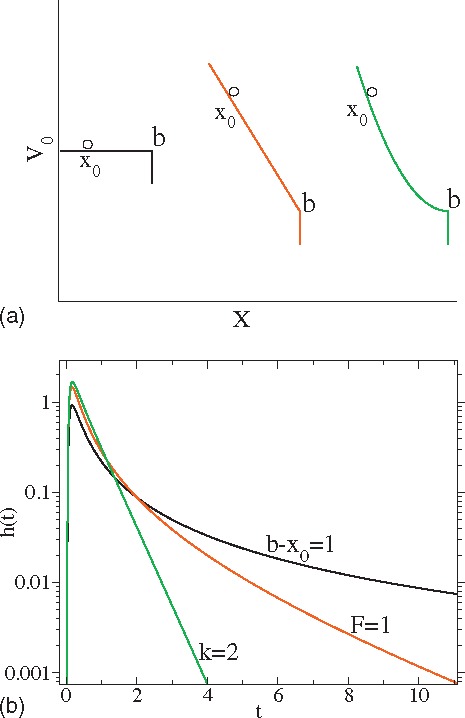
Several different potentials where we can solve the boundary value problem analytically. The particle starts from a position $x_0$ and disappear when passing over the point $b$. From left to right, $V_0\left(x\right)=0$, $V_0\left(x\right)=-Fx$, and $V_0\left(x\right)=\frac{1}{2}k{x}^2$.

IV. NUMERICAL SOLUTIONS

The total time-dependent interaction potential $V_0\left(x,t\right)$ of a protein molecule acted upon by a constant speed pulling force (exerted by either an atomic force microscope or laser tweezers) is taken to be

$$\beta V_0\left(x,t\right)=\beta V_m\left(x\right)+\frac{1}{2}{k}_s{\left(x-vt\right)}^2,$$ (15)

where $x$ is the fluctuating distance between the two pulling points, $V_m\left(x\right)$ is the intrinsic potential of mean force of the molecular system along the pulling coordinate, $v$ is the pulling speed, and $k_s$ is the effective spring constant of the pulling apparatus. An approximation used by Hummer and Szabo² and later by Dudko et al.^3,4 and Freund⁵ is to calculate a Kramers rate constant at time $t$, $K\left(t\right)$, using the instantaneous force at time $t$, an approximation that is probably valid only if the force varies slowly compared to the diffusional exploration of the instantaneous potential surface. This time-dependent rate constant is then used to estimate the survival probability so that

$$S\left(t\right)\simeq \text{exp}\left\{-{\int }_0^{t}K\left(\tau \right)d\tau \right\},$$ (16)

assuming first-order reaction kinetics, $dS\left(t\right)/dt=-K\left(t\right)S\left(t\right)$. The classical work of Kramers^13,19–21 states that the mean first passage time or the inverse of the rate constant for the barrier crossing problem of a time-independent potential $V_0\left(x\right)$ is given by

$$k_0^{-1}=\frac{1}{D}{\int }_{\text{b}}dx{e}^{\beta V_0\left(x\right)}{\int }_{\text{well}}dy{e}^{-\beta V_0\left(y\right)}.$$ (17)

Extending the Kramers result to the time-dependent potential in Eq. (15) when the pulling speed is slow, as suggested by Hummer and Szabo, yields the time-dependent mean first passage time

$$K{\left(t\right)}^{-1}=\frac{1}{D}{\int }_{\text{b}}dx{e}^{\beta V_0\left(x,t\right)}{\int }_{\text{well}}dy{e}^{-\beta V_0\left(y,t\right)}.$$ (18)

For a simple parabolic potential $\beta V_m\left(x\right)=\frac{1}{2}{k}_m{x}^2$, Eq. (18) can be evaluated approximately as (see details in the Appendix B)

$$K\left(t\right)\simeq \frac{D}{\sqrt{2\pi }}{k}^{3/2}\left(b-\frac{k_{s}vt}{k}\right)e^{-\left(1/2\right)k{\left(b-k_{s}vt/k\right)}^2},$$ (19)

where $k=k_m+k_s$. Following first-order kinetics, Eq. (16) reads

$$S\left(t\right)\simeq \text{exp}\left\{-\frac{D{k}^{3/2}}{\sqrt{2\pi }{k}_{s}v}\left[\text{exp}\left\{k_{s}vbt-\frac{1}{2}\frac{{\left(k_{s}vt\right)}^2}{k}\right\}-1\right]\right\}$$ (20)

which is the same as Eq. (16) in Ref. 2. The above procedure for handling this simple potential can be generalized to more complicated potentials as shown by Dudko et al.^3,4 and Freund.⁵ Freund has also shown that the first-order rate equation can be naturally derived from a thermodynamic approach. It has been noted that the underlying adiabatic approximation breaks down at extreme pulling speeds.³ It might be interesting to know whether their analytic formulas [Eq. (16) in Ref. 2, Eq. (4) in Ref. 3, Eq. (1) in Ref. 4, and Eqs. (10) and (14) in Ref. 5) are valid or not at conditions of slow intrinsic reaction rates (small $k_0$ or small $D$) or relatively larger pulling spring constant $k_s$.

For a complicated form of the potential of mean force $V_m\left(x\right)$, there is no analytical expression for either the first passage time distribution or the usual conditional probability in the absence of reaction. However, for the simple model potential $\beta V_m\left(x\right)=\frac{1}{2}{k}_m{x}^2$,^2–4 the usual conditional probability of this linear process has a Gaussian form (see details in Appendix C) (Ref. ¹²)

$$f_u^0\left(x,t\mid x_{\tau },\tau \right)=\frac{1}{\sqrt{2\pi {\sigma }_{t-\tau }}}\text{exp}\left\{-\frac{{\left(x-{\overline{x}}_{\tau ,t}\right)}^2}{2{\sigma }_{t-\tau }}\right\}$$ (21)

with the mean and variance

$${\overline{x}}_{\tau ,t}=x_{\tau }{e}^{-Dk\left(t-\tau \right)}+\frac{k_{s}v}{D{k}^2}\left(\left(1-Dk\tau \right)e^{-Dk\left(t-\tau \right)}+Dkt-1\right)$$ (22)

and

$${\sigma }_{t-\tau }=\left(1-e^{-2Dk\left(t-\tau \right)}\right)/k.$$ (23)

We are not able to solve the corresponding Smoluchowski Eq. (3) subject to the absorbing boundary condition (4) analytically to obtain the survival probability and the first passage time distribution. Instead, we evaluate the numerical solution of the integral Eq. (8) with the usual conditional probability of Eq. (21). Since the upper limit of the survival probability is

$$S\left(t\right)\le {\int }_{-\infty }^{b}dx{f}_u^0\left(x,t\mid x_0,0\right)=\frac{1}{2}\text{erfc}\left(-\frac{\left(b-{\overline{x}}_{0,t}\right)}{\sqrt{2{\sigma }_t}}\right),$$ (24)

Equation (8) might be solved iteratively by taking the upper limit as an ansatz. For general diffusive models having frequencies in the well $\left(x_0\right)$ and the transition $\left(b\right)$ regions, we might be able to use the analytical expression of the usual conditional probability corresponding to the harmonic potential for $f_u^0\left(x,t\mid x_0,0\right)$ as in Eq. (21) and use that corresponding to the inverted parabolic potential for $f_u^0\left(x,t\mid b,\tau \right)$ to solve Eq. (8) numerically.

We choose parameters $k_m=900\text{pN}/\text{nm}$, $k_s=10\text{pN}/\text{nm}$, and $b=0.42\text{nm}$ describing the unfolding of the I27 protein monomer.^2,7 The diffusion constant is chosen as either $D=0.044{\text{nm}}^2/\text{ms}$ or $D=0.0044{\text{nm}}^2/\text{ms}$ corresponding to the intrinsic reaction rate $k_0={10}^{-4}{\text{s}}^{-1}$ or $k_0={10}^{-5}{\text{s}}^{-1}$, respectively. Both intrinsic reaction rates are typical of biological systems. Figure 2 shows the results for the survival probability from direct simulations of the stochastic process Eq. (1) (black lines with circles), numerical solutions of the integral Eq. (8) (red), the approximate analytical form of Eq. (20) (green), and the upper limit Eq. (24) (blue lines with crosses). All green lines are terminated at $t$ such that ${\overline{x}}_{0,t}=b$ when the upper limit of the exact survival probability is equal to 1/2.

FIG. 2.

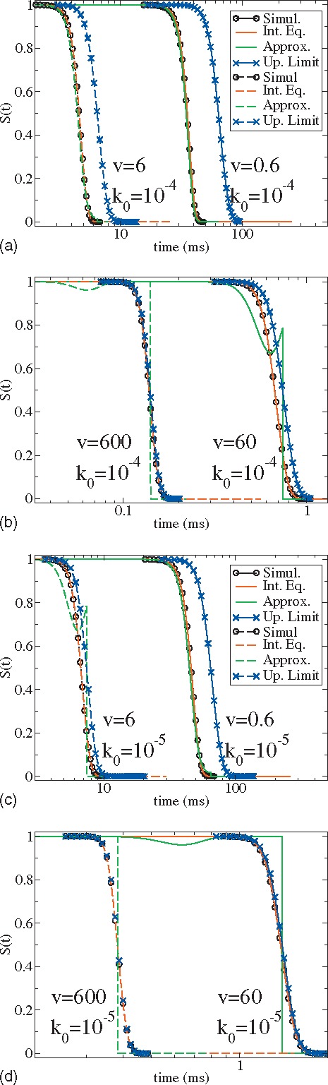
Survival probabilities at four different pulling speeds and two different diffusion constants calculated from several numerical and analytical methods. The $k_0$ rates are ${10}^{-4}{\text{s}}^{-1}$ (a and b) and ${10}^{-5}{\text{s}}^{-1}$ (c and d), respectively. Four pulling speeds $v=0.6$, 6.0, 60.0, and 600.0 nm/ms are studied. Black, red, green, and blue lines are numerical results from stochastic simulation, numerical results from the integral equation, approximated analytical results, and the Gaussian upper limit results, respectively. Black and red lines overlap in all graphs. Black, red, and blue dash lines in graphs (b) and (d) overlap. The pulling spring constant is $k_s=10\text{pN}/\text{nm}$ and $x_0=0$. We have put circles on the black lines (simulation results) and crosses on the blue lines (upper limit results) for a better view. Overlaps between black, red, and green lines at $v=0.6\text{nm}/\text{ms}$ (a and c) show that the adiabatic approximation works well at this experimental condition.

The overlap between the black and red lines confirms the exact relation between the usual conditional probability and the first passage time distribution at all pulling speeds and intrinsic reaction rates. The statistics and efficiency are much better when the numerical results are generated from the integral equation rather than from the stochastic simulation. As expected, the approximation underlying Eq. (16) is invalid at larger pulling speeds. Figures 2(a) and 2(c) shows that the previous theory [Eq. (16) in Ref. 2] starts to break down at relatively slower pulling speeds when the intrinsic rate of the system is relatively smaller $\left(k_0={10}^{-5}{\text{s}}^{-1}\right)$. In the limit of large pulling speeds, the survival probability approaches its upper limit indicating that the recrossing events make small contributions to the usual conditional probability. The analytical upper limit formula could be used to obtain estimates of thermodynamic and kinetic parameters when experimental data at large pulling speeds are available.

In experimental systems of forced protein unfolding where multimodules connected by molecular linkers are used instead of a single module, the effective pulling spring constant $k_s$ is relevant not only to the cantilever of the apparatus but also to the properties of the molecular linker and the module itself. In a recent experiment of unfolding I27 domain by Harris and Kiang,²² the spring constant of the cantilever is $50\text{pN}/\text{nm}$. As suggested by Hummer and Szabo,² a rough estimate from the slope of the force-extension curves before rupture [Fig. 1b in Ref. 22] yields the effective pulling spring constants $k_s=10–20\text{pN}/\text{nm}$. Figure 3 shows our calculations of the survival probabilities at $k_s=50\text{pN}/\text{nm}$ and $k_0={10}^{-4}{\text{s}}^{-1}$. Comparison between Figs. 2(a) and 3 reveals that the rupture time significantly reduces as $k_s$ increases from 10 to 50 pN/nm. Thus the approximated analytical theory based on Eq. (16) become less applicable at a larger $k_s$.

FIG. 3.

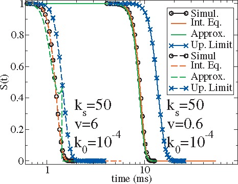
Survival probability at two different pulling speeds, similar to Fig. 2(a) but for the pulling spring constant $k_s=50\text{pN}/\text{nm}$. Black and red lines overlap. All the labels are the same as in Fig. 2.

Experimentalists usually report the distribution and average of the force at rupture for different pulling speeds determined from the integration and the differentiation of the measured survival probability

$$\overline{F}=-k_s\left(b-v{\int }_0^{\infty }d\tau \tau h\left(\tau \right)\right)=-k_s\left(b-v{\int }_0^{\infty }S\left(t\right)dt\right)$$ (25)

and

$$p\left(F\right)=\frac{1}{k_{s}v}h\left(t\right){\mid }_{t=\left(F+k_{s}b\right)/\left(k_{s}v\right)}.$$ (26)

As shown in Figs. 2 and 3, the areas under the survival probability from the exact solution (black or red) and the approximated analytical solution (green) are almost equal for all cases investigated. Thus the previous analytical expressions based on Eq. (16) are still approximately valid when fitting the average force as a function of the pulling speeds. However the deviations of the rupture force distribution are severe especially at larger pulling speeds $v$, slower intrinsic rates $k_0$, or larger effective pulling spring constants $k_s$. A comparison among the predictions of the approximate theory, the stochastic simulation results, and the exact results determined from the integral equation for varying $v$, $k_0$, and $k_s$ is shown in Fig. 4. Clearly, to fit the experimental data at relatively larger pulling speeds, larger pulling spring constant or smaller intrinsic reaction rates, it is quite necessary to obtain the numerical results from the integral equations for the specific model and not from the approximate theory.

FIG. 4.

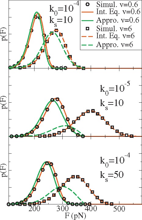
Rupture force distributions at two different pulling speeds, intrinsic rates, and effect pulling constants calculated from stochastic simulation (black circles or squares), the integral equation (red), and the approximated analytical theory (green). See Eqs. (8), (16), and (26).

V. CONCLUSION

We have presented an integral equation connecting the usual conditional probability in the absence of reaction and the first passage time distribution and have found analytical solutions of this equation for the cases of free and biased particle diffusion in time-independent potentials. The long time tail $t^{-3/2}$ in the case of free diffusion rapidly vanishes as the diffusion is biased by a linear or harmonic potential. For diffusion in a time-dependent potential of biological interest, we solved the integral equations numerically and compared the results with both stochastic simulations and a previously developed approximate theory bases on an adiabatic approximation. We found that iteration from the upper bound of the survival probability is useful for extracting kinetic and thermodynamic parameters ($k_0$, $k_s$, $b$, and $k_m$) from biological experimental data at extreme pulling speeds. We see that the approximated analytical formulas for the rupture force distribution based on the Kramers theory and the adiabatic assumption are likely to break down at larger pulling speeds, larger pulling spring constants, or smaller intrinsic reaction rates. Once these thermodynamic and kinetic parameters are estimated or extracted either by fitting the average rupture force to the approximate analytical theories or by fitting the survival probability at extreme pulling speeds to their upper limits, our numerical treatment, based on the integral equation, can be immediately extended to fit experimental rupture force distributions at all pulling speeds and to further verify the validity of the parameters.

In this paper we provide a simple numerical procedure, based on an iterative solution of an integral equation for the survival probability, to extend previous methods for fitting the force distribution for arbitrary conditions of pulling speeds, cantilever spring constants, and intrinsic reaction rates. However, we should point out that the underlying assumption that the rupture kinetics can be described by a Langevin process in its spatial diffusion limit might not be generally true. Recently, simulations and experiments have revealed that water insertion plays a significant role in the single-molecule kinetics of the forced unfolding of ubiquitin.^23,24 When the unfolding kinetics depends on the number of inserted water molecules, there might not exist a well-defined transition state, but rather a broad distribution of transition states which give rise to static disorder and nonexponential decay. Further investigation will be required to determine whether a diffusive model with an effective diffusion constant, fixed barrier height, and transition distance is still valid for the description of these biological rupture experiments.

Note added in proof. After our paper was accepted for publication, Attila Szabo told us that our integral equation Eq. (6) is similar to an established equation found in Schrødinger's 1915 paper.²⁵ Our self-consistent integral Eq. (8) is therefore a natural extension of Schrødinger's work in 1915.

APPENDIX A: ANALYTICAL SOLUTIONS FOR THE FIRST PASSAGE TIME DISTRIBUTION FOR THREE MODEL POTENTIALS

We derive the analytical solutions of the integral Eqs. (7) and (8) for the simple potentials illustrated in Fig. 1(a) in this appendix. For $V_0\left(x\right)=0$, we find

$${\int }_{-\infty }^{b}dx{f}_u^0\left(x,t\mid b,\tau \right)={\int }_{-\infty }^{b}dx\frac{1}{\sqrt{4\pi D\left(t-\tau \right)}}\text{exp}\left\{-\frac{{\left(x-b\right)}^2}{4D\left(t-\tau \right)}\right\}=\frac{1}{2}.$$ (A1)

Equation (8) thus takes a remarkably simple form

$$S\left(t\right)={\int }_{-\infty }^{b}dx{f}_u^0\left(x,t\mid x_0,0\right)-\frac{1}{2}\left(1-S\left(t\right)\right).$$ (A2)

The analytical solution of the survival probability is

$$S\left(t\right)=2{\int }_{-\infty }^{b}dx{f}_u^0\left(x,t\mid x_0,0\right)-1$$ (A3)

and its differentiation gives the first passage time distribution

$$h\left(t\right)=-\frac{dS\left(t\right)}{dt}=\frac{\left(b-x_0\right)}{\sqrt{4\pi D{t}^3}}\text{exp}\left\{-\frac{{\left(b-x_0\right)}^2}{4Dt}\right\}$$ (A4)

which is the same as Eq. (10). Alternatively, the Laplace transform of Eq. (7) in the case of free particle diffusion yields

$$\frac{1}{\sqrt{4Ds}}\text{exp}\left\{-\frac{\left(x-b\right)\sqrt{s}}{\sqrt{D}}\right\}\tilde{h}\left(s\right)=\frac{1}{\sqrt{4Ds}}\text{exp}\left\{-\frac{\left(x-x_0\right)\sqrt{s}}{\sqrt{D}}\right\}.$$ (A5)

Immediately we have

$$\tilde{h}\left(s\right)=\text{exp}\left\{-\frac{\left(b-x_0\right)\sqrt{s}}{\sqrt{D}}\right\}$$ (A6)

and its inverse Laplace transform gives the same result as in Eq. (A4).

We further rewrite Eq. (7) as

$${\int }_0^{t}d\tau h\left(\tau \right)\frac{f_u^0\left(x,t\mid b,\tau \right)}{f_u^0\left(x,t\mid x_0,0\right)}=1.$$ (A7)

$h\left(\tau \right)$ implicitly depends on $b$ and $x_0$ only and it has to be chosen such that the integration is 1 for any $x\ge b$. For the case of $V_0\left(x\right)=0$,

$$\frac{f_u^0\left(x,t\mid b,\tau \right)}{f_u^0\left(x,t\mid x_0,0\right)}=\frac{\sqrt{t}}{\sqrt{t-\tau }}\text{exp}\left\{-\frac{{\left(x-b\right)}^2}{4D\left(t-\tau \right)}+\frac{{\left(x-x_0\right)}^2}{4Dt}\right\}.$$ (A8)

The exponential part of $h\left(t\right)$ as in Eq. (A4) completes a parabolic form inside the exponential

$$-\frac{{\left(x-b\right)}^2}{4D\left(t-\tau \right)}+\frac{{\left(x-x_0\right)}^2}{4Dt}-\frac{{\left(b-x_0\right)}^2}{4D\tau }=-\frac{{\left[\left(x-x_0\right)\tau -\left(b-x_0\right)t\right]}^2}{4Dt\tau \left(t-\tau \right)}.$$ (A9)

After a substitution of the integration dummy variable $y=\sqrt{t-\tau }/\sqrt{t\tau }$, Eq. (A7) becomes a known result

$${\int }_0^{\infty }dy\frac{2d}{\sqrt{\pi }}\text{exp}\left\{-d^2{\left[y-\frac{c}{y}\right]}^2\right\}=1,$$ (A10)

where $c=\left(x-b\right)/\left[t\left(b-x_0\right)\right]$ and $d=\left(b-x_0\right)/\left(4D\right)$ are both positive parameters independent of $y$. The derivation from Eq. (A7) to Eq. (A10) provides a simple method through which we can guess the form of $h\left(t\right)$ such that the integration does not depend on the parameter $x$, for general cases of the biased diffusions.

For $V_0\left(x\right)=-Fx$, the usual conditional probability of the linear process takes the form of Eq. (11). We might make the following analogy:

$$x\leftrightarrow x-FDt,b\leftrightarrow b-FD\tau ,x_0\leftrightarrow x_0.$$

When we choose $h\left(\tau \right)\sim \text{exp}\left\{-{\left(b-FD\tau -x_0\right)}^2/\left(4D\tau \right)\right\}$, the analog expression inside the exponential of the integral is

$$-\frac{{\left[\left(x-x_0\right)\tau -\left(b-x_0\right)t\right]}^2}{4Dt\tau \left(t-\tau \right)}\leftrightarrow -\frac{{\left[\left(x-FDt-x_0\right)\tau -\left(b-FD\tau -x_0\right)t\right]}^2}{4Dt\tau \left(t-\tau \right)}=-\frac{{\left[\left(x-x_0\right)\tau -\left(b-x_0\right)t\right]}^2}{4Dt\tau \left(t-\tau \right)}$$ (A11)

which is the same as in the case of the free particle diffusion. Therefore taking the same coefficient as in Eq. (A4) arrives at Eq. (A10) after the substitution from $\tau$ to $y$. We thus find the result in Eq. (12)

$$h\left(t\right)=\frac{\left(b-x_0\right)}{\sqrt{4\pi D{t}^3}}\text{exp}\left\{-\frac{{\left(b-FDt-x_0\right)}^2}{4Dt}\right\}.$$ (A12)

For $V_0\left(x\right)=\frac{1}{2}k{x}^2$, we apply the following analogy:

$$x\leftrightarrow x{e}^{Dkt},b\leftrightarrow b{e}^{Dk\tau },x_0\leftrightarrow x_0,$$

$$t\leftrightarrow \frac{e^{2Dkt}-1}{2Dk}=\widehat{t},$$

$$\tau \leftrightarrow \frac{e^{2Dk\tau }-1}{2Dk}=\widehat{\tau },t-\tau \leftrightarrow \frac{e^{2Dkt}-e^{2Dk\tau }}{2Dk}=\widehat{t}-\widehat{\tau }.$$

The corresponding analog expression inside the exponential reads

$$-\frac{{\left[\left(x-x_0\right)\tau -\left(b-x_0\right)t\right]}^2}{4Dt\tau \left(t-\tau \right)}\leftrightarrow -\frac{{\left[\left(x{e}^{Dkt}-x_0\right)\widehat{\tau }-\left(b{e}^{Dk\tau }-x_0\right)\widehat{t}\right]}^2}{4D\widehat{t}\widehat{\tau }\left(\widehat{t}-\widehat{\tau }\right)}.$$ (A13)

In this case, it might not be easy to choose an appropriate coefficient of $h\left(\tau \right)$ such that the integral is independent of $x$. However, for $b=0$, it is straightforward to have

$$h\left(\tau \right)=\frac{d\widehat{\tau }}{d\tau }\frac{b-x_0}{\sqrt{4\pi D{\widehat{\tau }}^3}}\text{exp}\left\{-\frac{{\left(b{e}^{Dk\tau }-x_0\right)}^2}{4D\widehat{\tau }}\right\}=\frac{e^{2Dk\tau }\left|x_0\right|}{\sqrt{4\pi D{\widehat{\tau }}^3}}\text{exp}\left\{-\frac{x_0^2}{4D\widehat{\tau }}\right\},$$ (A14)

which is equivalent to Eq. (14). We thus complete the analytical solutions for the three simple potentials in Fig. 1.

APPENDIX B: ANALYTICAL SOLUTION FOR A TIME-DEPENDENT BARRIER CROSSING PROBLEM USING KRAMERS THEORY AND THE ADIABATIC APPROXIMATION

We explain the derivation of Eq. (19) in this appendix. For a time-independent potential $\beta V_0\left(x,t\right)=k_m{x}^2/2$, the integral over the well appearing in the right hand side (rhs) of Eq. (17) is bounded as

$$\frac{1}{2}\frac{\sqrt{2\pi }}{\sqrt{k_m}}={\int }_{-\infty }^{0}dy{e}^{-\left(1/2\right)k_m{y}^2}\le {\int }_{\text{well}}dy{e}^{-\left(1/2\right)k_m{y}^2}\le {\int }_{-\infty }^{+\infty }dy{e}^{-\left(1/2\right)k_m{y}^2}=\frac{\sqrt{2\pi }}{\sqrt{k_m}}.$$ (B1)

The integral over the barrier of the rhs of Eq. (17) is written as

$${\int }_0^{b}dx{e}^{-\left(1/2\right)k_m{x}^2}=e^{\left(1/2\right)k_m{b}^2}{\int }_0^{b}dx{e}^{\left(k_m/2\right)\left(x^2-b^2\right)}.$$ (B2)

For $0<x<b$ and $2b\left(x-b\right)<\left(x^2-b^2\right)<b\left(x-b\right)$, the above integral is bounded as

$${\int }_0^{b}dx{e}^{-\left(1/2\right)k_m{x}^2}\le e^{\left(1/2\right)k_m{b}^2}{\int }_0^{b}dx{e}^{-\left(1/2\right)k_{m}b\left(x-b\right)}=e^{\left(1/2\right)k_m{b}^2}\frac{2}{k_{m}b}\left(1-e^{-\left(1/2\right)k_m{b}^2}\right)$$ (B3)

and

$${\int }_0^{b}dx{e}^{-\left(1/2\right)k_m{x}^2}\ge e^{\left(1/2\right)k_m{b}^2}{\int }_0^{b}dx{e}^{-k_{m}b\left(x-b\right)}=e^{\left(1/2\right)k_m{b}^2}\frac{1}{k_{m}b}\left(1-e^{-k_m{b}^2}\right).$$ (B4)

The Kramers rate in Eq. (17), dependent on $k_m$ and $b$ is thus bounded as

$$k_0^{-1}\left(k_m,b\right)\ge \frac{1}{D}\frac{1}{2}\frac{\sqrt{2\pi }}{\sqrt{k_m}}\frac{1}{k_{m}b}{e}^{\left(1/2\right)k_m{b}^2}\left(1-e^{-k_m{b}^2}\right)$$ (B5)

and

$$k_0^{-1}\left(k_m,b\right)\le \frac{1}{D}\frac{\sqrt{2\pi }}{\sqrt{k_m}}\frac{2}{k_{m}b}{e}^{\left(1/2\right)k_m{b}^2}\left(1-e^{-\left(1/2\right)k_m{b}^2}\right).$$ (B6)

In case of $k_m{b}^2⪢1$, we might take the middle value

$$k_0^{-1}\left(k_m,b\right)\simeq \frac{1}{D}\frac{\sqrt{2\pi }}{\sqrt{k_m}}\frac{1}{k_{m}b}{e}^{\left(1/2\right)k_m{b}^2}$$ (B7)

which is Eq. (11) in ref. 2. For the time-dependent potential,

$$\beta V_0\left(x,t\right)=\frac{1}{2}{k}_m{x}^2+\frac{1}{2}{k}_s{\left(x-vt\right)}^2=\frac{1}{2}k{\left(x-\frac{k_{s}vt}{k}\right)}^2+\frac{1}{2}\frac{k_m{k}_s{v}^2{t}^2}{k}=\frac{1}{2}k{\left(x-s\right)}^2+\frac{1}{2}\frac{k{k}_m{s}^2}{k_s},$$ (B8)

where $s=k_{s}vt/k$ is a parameter independent of $x$. Based on the result of Eq. (B7), Eq. (19) is evaluated as

$$K{\left(t\right)}^{-1}=k_0^{-1}\left(k,b-s\right)\simeq \frac{1}{D}\frac{\sqrt{2\pi }}{\sqrt{k}}\frac{1}{k\left(b-s\right)}{e}^{\left(1/2\right)k{\left(b-s\right)}^2}$$ (B9)

which is the same as Eq. (19).

APPENDIX C: TIME-DEPENDENT GREEN'S FUNCTION FOR A LINEAR STOCHASTIC PROCESS IN THE ABSENCE OF AN ABSORBING BOUNDARY

We explain the derivation of Eqs. (21)–(23). There are many alternative methods to solve the stochastic differential equation described by Eq. (1) in a time-dependent harmonic potential. One method is to use the solution for the Ornstein–Uhlenbeck process given on page 238 of Ref. 12. We indicate here a similar approach for the simple case of one-dimensional system in order to illustrate this method. The Markov process of interest can be rewritten as

$$\frac{du}{dt}=-D\left(k_m+k_s\right)u+D{k}_{s}vt+\sqrt{2D}\frac{d\omega }{dt},$$ (C1)

where $\omega \left(t\right)$ denotes a Gaussian random variable with mean 0 and variance $t$. Considering the initial condition $u\left(\tau \right)=x_{\tau }$ with probability of 1, direct integration gives the solution to the first order differential equation (C1) as

$$u\left(t\right)=x_{\tau }{e}^{-Dk\left(t-\tau \right)}+{\int }_{\tau }^t{e}^{-Dk\left(t-t^{\prime }\right)}\left(D{k}_{s}v{t}^{\prime }+\sqrt{2D}\frac{d\omega }{d{t}^{\prime }}\right)d{t}^{\prime }=x_{\tau }{e}^{-Dk\left(t-\tau \right)}+\frac{k_{s}v}{D{k}^2}\left(\left(1-Dk\tau \right)e^{-Dk\left(t-\tau \right)}+Dkt-1\right)+\sqrt{2D}{\int }_{\tau }^t{e}^{-Dk\left(t-t^{\prime }\right)}d\omega ={\overline{x}}_{\tau ,t}+\sqrt{2D}\underset{\Delta t\to 0}{\text{lim}}\sum _{i=1}^N{e}^{-Dk\left(t-\tau -\left(i-1\right)\Delta t\right)}{\omega }_i\left(\Delta t\right),$$ (C2)

where ${\overline{x}}_{\tau ,t}$ is the same as in Eq. (22). ${\omega }_i\left(\Delta t\right)$ are treated as independent Gaussian random variables with variance $\Delta t$ and $t=\tau +N\Delta t$. The variance of the random variable $u\left(t\right)$ is

$${\sigma }_{t-\tau }=2D{e}^{-2Dk\left(t-\tau \right)}\underset{\Delta t\to 0}{\text{lim}}\Delta t\frac{1-e^{2Dk\left(t-\tau \right)}}{1-e^{2Dk\Delta t}}=\frac{1-e^{-2Dk\left(t-\tau \right)}}{k}$$ (C3)

which is the expression given in Eq. (23).

REFERENCES

- 1.Redner S., A Guide to First-Passage Processes (Cambridge University Press, Cambridge, 2001). 10.1017/CBO9780511606014 [DOI] [Google Scholar]
- 2.Hummer G. and Szabo A., Biophys. J. 85, 5 (2003). 10.1016/S0006-3495(03)74449-X [DOI] [PMC free article] [PubMed] [Google Scholar]
- 3.Dudko O. K., Hummer G., and Szabo A., Phys. Rev. Lett. 96, 108101 (2006). 10.1103/PhysRevLett.96.108101 [DOI] [PubMed] [Google Scholar]
- 4.Dudko O. K., Hummer G., and Szabo A., Proc. Natl. Acad. Sci. U.S.A. 105, 15755 (2008). 10.1073/pnas.0806085105 [DOI] [PMC free article] [PubMed] [Google Scholar]
- 5.Freund L. B., Proc. Natl. Acad. Sci. U.S.A. 106, 8818 (2009). 10.1073/pnas.0903003106 [DOI] [PMC free article] [PubMed] [Google Scholar]
- 6.Dudko O. K., Filippov A. E., Klafter J., and Urbakh M., Proc. Natl. Acad. Sci. U.S.A. 100, 11378 (2003). 10.1073/pnas.1534554100 [DOI] [PMC free article] [PubMed] [Google Scholar]
- 7.Carrion-Vazquez M., Oberhauser A. F., Fowler S. B., Marszalek P. E., Broedel S. E., Clarke J., and Fernandez J. M., Proc. Natl. Acad. Sci. U.S.A. 96, 3694 (1999). 10.1073/pnas.96.7.3694 [DOI] [PMC free article] [PubMed] [Google Scholar]
- 8.Schlierf M. and Rief M., Biophys. J. 90, L33 (2006). 10.1529/biophysj.105.077982 [DOI] [PMC free article] [PubMed] [Google Scholar]
- 9.Mathé J., Visram H., Viasnoff V., Rabin Y., and Meller A., Biophys. J. 87, 3205 (2004). 10.1529/biophysj.104.047274 [DOI] [PMC free article] [PubMed] [Google Scholar]
- 10.Chandrasekhar S., Rev. Mod. Phys. 15, 1 (1943). 10.1103/RevModPhys.15.1 [DOI] [Google Scholar]
- 11.Montroll E. W. and Weiss G. H., J. Math. Phys. 6, 167 (1965). 10.1063/1.1704269 [DOI] [Google Scholar]
- 12.Risken H., The Fokker-Planck Equation (Springer-Verlag, Berlin, 1989). [Google Scholar]
- 13.Kramers H. A., Physica (Amsterdam) 7, 284 (1940). 10.1016/S0031-8914(40)90098-2 [DOI] [Google Scholar]
- 14.Szabo A., Lamm G., and Weiss G. H., J. Stat. Phys. 34, 225 (1984). 10.1007/BF01770356 [DOI] [Google Scholar]
- 15.Bicout D. J. and Szabo A., J. Chem. Phys. 106, 10292 (1997). 10.1063/1.474066 [DOI] [Google Scholar]
- 16.Szabo A., Schulten K., and Schulten Z., J. Chem. Phys. 72, 4350 (1980). 10.1063/1.439715 [DOI] [Google Scholar]
- 17.Gerstein G. L. and Mandelbrot B., Biophys. J. 4, 41 (1964). 10.1016/S0006-3495(64)86768-0 [DOI] [PMC free article] [PubMed] [Google Scholar]
- 18.Fienberg S. E., Biometrics 30, 399 (1974). 10.2307/2529198 [DOI] [PubMed] [Google Scholar]
- 19.Berne B. J., Borkovec M., and Straub J. E., J. Phys. Chem. 92, 3711 (1988). 10.1021/j100324a007 [DOI] [Google Scholar]
- 20.Hänggi P., Talkner P., and Borkovec M., Rev. Mod. Phys. 62, 251 (1990). 10.1103/RevModPhys.62.251 [DOI] [Google Scholar]
- 21.Zwanzig R., Nonequilibrium Statistical Mechanics (Oxford University Press, New York, 2001). [Google Scholar]
- 22.Harris N. C. and Kiang C. -H., Phys. Rev. E 79, 041912 (2009). 10.1103/PhysRevE.79.041912 [DOI] [PubMed] [Google Scholar]
- 23.Kuo T. -L., Garcia-Manyes S., Li J., Barel I., Lu H., Berne B., Urbakh M., Klafter J., and Fernandez J. M., Proc. Natl. Acad. Sci. U.S.A. 107, 11336 (2010). 10.1073/pnas.1006517107 [DOI] [PMC free article] [PubMed] [Google Scholar]
- 24.Li J., Fernandez J. M., and Berne B. J., “Water's role in the force induced unfolding of ubiquitin,” Proc. Natl. Acad. Sci. U.S.A. (submitted). [DOI] [PMC free article] [PubMed]
- 25.Schrødinger E., Phys. Z 16, 289 (1915). Also see [Google Scholar]; Lumpkin O., Phys. Rev. A 51, 2758 (1995). 10.1103/PhysRevA.51.2758 [DOI] [PubMed] [Google Scholar]