Inferring changepoint times of medial temporal lobe morphometric change in preclinical Alzheimer's disease

Abstract

This paper uses diffeomorphometry methods to quantify the order in which statistically significant morphometric change occurs in three medial temporal lobe regions, the amygdala, entorhinal cortex (ERC), and hippocampus among subjects with symptomatic and preclinical Alzheimer's disease (AD). Magnetic resonance imaging scans were examined in subjects who were cognitively normal at baseline, some of whom subsequently developed clinical symptoms of AD. The images were mapped to a common template, using shape-based diffeomorphometry. The multidimensional shape markers indexed through the temporal lobe structures were modeled using a changepoint model with explicit parameters, specifying the number of years preceding clinical symptom onset. Our model assumes that the atrophy rate of a considered brain structure increases years before detectable symptoms.

The results demonstrate that the atrophy changepoint in the ERC occurs first, indicating significant change 8–10 years prior to onset, followed by the hippocampus, 2–4 years prior to onset, followed by the amygdala, 3 years prior to onset. The ERC is significant bilaterally, in both our local and global measures, with estimates of ERC surface area loss of 2.4% (left side) and 1.6% (right side) annually. The same changepoint model for ERC volume gives 3.0% and 2.7% on the left and right sides, respectively. Understanding the order in which changes in the brain occur during preclinical AD may assist in the design of intervention trials aimed at slowing the evolution of the disease.

Highlights

• •We use diffeomorphometry to quantify the order in which statistically significant morphometric change occurs in three medial temporal lobe regions, the amygdala, entorhinal cortex (ERC), and hippocampus among subjects with symptomatic and preclinical Alzheimer's disease (AD).
• •We introduce a model on anatomical shape change in which changepoint is inferred, taking place some period of time before cognitive onset of AD.
• •The analysis uses a dataset arising from the BIOCARD study, in which all subjects were cognitively normal at baseline, some of whom subsequently developed clinical symptoms of AD.
• •The results demonstrate that the atrophy changepoint in the ERC occurs first, indicating significant change 8-10 years prior to onset, followed by hippocampus, 2-4 years prior to onset, followed by amygdala, 3 years prior to onset.
• •The ERC is significant bilaterally, in both our local and global measures, with estimates of ERC surface area loss of 2.4% (left side) and 1.6% (right side) annually.
• •Understanding the order in which changes in the brain occur during preclinical AD may assist in the design of intervention trials aimed at slowing the evolution of the disease.

1. Introduction

Brain imaging and MRI studies have substantially advanced our knowledge of regional brain atrophy in Alzheimer's disease (AD). Magnetic resonance imaging (MRI) measures are an indirect reflection of the neuronal injury that occurs in the brain as the AD pathophysiological process evolves. In the initial stages of AD, atrophy on MRI appears to have a predilection for the brain regions with heavy deposits of neurofibrillary tangles (Braak and Braak, 1991; Arnold et al., 1991; Price and Morris, 1999). Consistent with this pattern, the volume of the entorhinal cortex, the hippocampus and other medial temporal lobe structures has been shown to discriminate between patients with AD dementia and controls, and between subjects with mild cognitive impairment (MCI) and controls, and to be associated with time to progress from MCI to AD dementia (Kantarci and Jack, 2003; Atiya et al., 2003). Longitudinal MRI data in cognitively normal individuals who have progressed to mild impairment (i.e., preclinical AD) is limited but suggests that volumetric measures of medial temporal lobe regions may predict progression from normal cognition to mild impairment. Differences in atrophy rate of the entorhinal cortex (Jack et al., 2004; Miller et al., 2013a), the hippocampus or subvolumes of the hippocampus (Jack et al., 2004; Apostolova et al., 2010) and ventricular volume (Carlson et al., 2008) have been demonstrated during preclinical AD. It has also been demonstrated that baseline measures of the hippocampus and amygdala in controls predict subsequent development of MCI (den Heijer et al., 2006), with hippocampus shape differences being reported among controls who subsequently developed cognitive impairment (Rusinek et al., 2003; Chiang et al., 2009; Csernansky et al., 2005; den Heijer et al., 2006; Thambisetty et al., 2010).

Methods of statistical analysis based on diffeomorphometry for studying normal age-related changes in subcortical nuclei and in a number of other diseases have already been enlightening (Qiu et al., 2010; Qiu et al., 2009a; Csernansky et al., 1998; Csernansky et al., 2000; Wang et al., 2007; Ashburner et al., 2003; Thompson et al., 2004; Younes et al., 2012; Tang et al., 2013). This study follows our previous study in the same subject population (Miller et al., 2013a) in which we used diffeomorphometry to measure subregional atrophy in three structures of the temporal lobe, entorhinal cortex (ERC), hippocampus and amygdala and demonstrated statistically significant changes in brain structures during preclinical AD. These prior results are consistent with histopathological findings that suggest that these regions are affected during the earliest phase of AD (Arriagada et al., 1992; Herzog and Kemper, 1980; Scott et al., 1991; Scott et al., 1992; Tsuchiya and Kosaka, 1990). This approach allows for a fine-scale, high-dimensional, analysis of non-uniform change patterns in the structures, and complements coarser low-dimensional measures, like structure volume.

The study described here focuses on the temporal order of atrophy of the same three structures. The diffeomorphometry pipeline follows our general pattern (Younes et al., 2012; Tang et al., 2013; Miller et al., 2013a), first involving an initial coarse rigid alignment phase followed by a high-dimensional template-matching phase. This registers all shape morphometry to a single template coordinate system, which is centered to the population, producing a high-dimensional representation of the data in a coordinate system in which each coordinate is directly comparable across the population. The statistical analysis uses multivariate models including a nonlinear component defining a changepoint in atrophy over time, with significance assessed while taking multiple comparisons into account. The introduction of the changepoint model offers the opportunity to quantify the temporal ordering of morphometric changes among these temporal lobe structures in preclinical AD (i.e., the ERC, hippocampus and amygdala), which we have already found to be discriminating in these groups of temporal lobe structures in preclinical AD (Miller et al., 2013a). No modeling of the order in years preceding clinical onset has yet been explicitly modeled or demonstrated to our knowledge.

2. Subjects and data acquisition

2.1. Study design

The overall study (known as the BIOCARD study), is a longitudinal characterization of individuals funded jointly by the National Institutes on Aging (NIA) and Mental Health (NIMH). All BIOCARD subjects were cognitively normal when recruited with mean age at baseline of 57.1 years. Scans were acquired during the period 1995–2005. A total of 805 scans have been collected during the 10-year period. The participants have now been followed for up to 18 years.

A total of 354 individuals were initially enrolled in the study. Recruitment was conducted by the staff of the Geriatric Psychiatry branch of the Intramural Program of the NIMH, beginning in 1995 and ending in 2005. Subjects were recruited via printed advertisements, articles in local or national media, informational lectures, or word-of-mouth. The study was designed to recruit and follow a cohort of cognitively normal individuals who were primarily in middle age. By design, approximately three-quarters of the participants had a first-degree relative with dementia of the Alzheimer type. The overarching goal was to identify variables among cognitively normal individuals that could predict the subsequent development of mild to moderate symptoms of AD. Subjects were administered a comprehensive neuropsychological battery annually. MRI scans, cerebrospinal fluid (CSF), and blood specimens were obtained every 2 years. The study was initiated at the Clinical Center of the National Institutes of Health (NIH) in 1995, and was stopped in 2005. In 2009, our research team was funded to re-establish the cohort, continue the annual clinical and cognitive assessments, collect blood, and evaluate the previously acquired MRI scans, CSF and blood specimens.

At baseline, all participants completed a comprehensive evaluation at the NIH. This evaluation consisted of a physical and neurological examination, an electrocardiogram, standard laboratory studies (e.g., complete blood count, vitamin B12, thyroid function), and neuropsychological testing. Individuals were excluded from participation if they were cognitively impaired, as determined by cognitive testing, or had significant medical problems such as severe cerebrovascular disease, epilepsy or alcohol or drug abuse. Five subjects did not meet the entry criteria and were excluded at baseline, leaving a total of 349 participants followed over time.

2.2. MRI assessments

MRI scans were obtained on 335 participants at baseline. An additional 470 scans were obtained in subsequent years for a total of 805 scans. The mean interval between scan acquisitions on follow-up was 2.02 years. The MRI scans acquired at the NIH were obtained using a standard multi-modal protocol using GE 1.5 T scanner. The scanning protocol included localizer scans, axial FSE sequence (TR = 4250 ms, TE = 108 ms, FOV = 512 × 512, thickness/gap = 5.0/0.0 mm, flip angle = 90°, 28 slices), axial FLAIR sequence (TR = 9002 ms, TE = 157.5 ms, FOV = 256 × 256, thickness/gap = 5.0/0.0 mm, flip angle = 90°, 28 slices), coronal SPGR (spoiled gradient echo) sequence (TR = 24 ms, TE = 2 ms, FOV = 256 × 256, thickness/gap = 2.0/0.0 mm, flip angle = 20°, 124 slices), sagittal SPGR sequence (TR = 24 ms, TE = 3 ms, FOV = 256 × 256, thickness/gap 1.5/0.0 mm, flip angle = 45°, 124 slices).

2.3. Clinical and cognitive assessments

The clinical and cognitive assessments of the participants have been described elsewhere (Soldan et al., 2013). The cognitive assessment consisted of a neuropsychological battery covering all major cognitive domains (i.e., memory, executive function, language, spatial ability, attention and processing speed). A clinical assessment was also conducted annually. Since the study has been conducted by the current research team, this has included the following: a physical and neurological examination, record of medication use, behavioral and mood assessments (Cummings et al., 1994; Yesavage et al., 1982), family history of dementia, history of symptom onset, and a clinical dementia rating (CDR), based on a semi-structured interview (Hughes et al., 1982; Morris, 1993). The clinical assessments given at the NIH covered similar domains. The diagnostic procedures in this study are comparable to those used in the Alzheimer's disease research centers program, funded by the National Institute on Aging. This involves a two-step process by which a decision is first made about whether the subject is normal, mildly impaired or demented (based on the clinical history, medical, neurologic and psychiatric evaluations and the cognitive testing), and then (if the subject is judged not to be normal) the likely cause(s) of the cognitive impairment is determined. This same diagnostic process was applied retrospectively to participants who had become cognitively impaired while the study was being conducted at the NIH, but who (by the time the study had been re-established) were either moderate-to-severely impaired or were no longer living. It should be noted that the estimated age-of-onset of clinical symptoms, which is the primary outcome in these analyses, was established on the basis of clinical information elicited during the CDR interview by the clinician who evaluated the subject (or on the basis of clinical notes in the record), and re-confirmed during the consensus conference.

2.4. MRI scans available for analysis

Some subjects were removed from the analysis for uncertain diagnostic (impairment not categorized as MCI) and several scans had to be removed because they contained significant artifacts that prevented structure segmentation. The dataset used in this study includes MRI scans from 296 subjects, of which 230 individuals remained cognitively normal and 66 developed cognitive impairment and were diagnosed with MCI (of these, 17 subsequently progressed to AD dementia). The average number of scans per subject is 2.2 among the 230 controls and 2.5 among the 66 who progressed to MCI or AD dementia, for a total number of 661 scans overall used in this study. Table 1 summarizes demographic data for the subjects that were the focus of our analyses.

Table 1.

Participant characteristics at baseline and follow-up stratified by outcome status.

Variable	Control group (N = 230)	MCI or AD before 2005 (N = 15)	MCI or AD after 2005 (N = 51)	Combined MCI/AD (N = 66)
Age at entry, mean number of years (SD)	55.3 (9.8)	66 (7.5)	62.4 (11.4)	63.3 (10.8)
Gender, females (%)	61%	53%	49%	50%

It should be noted that our dataset differs from the one used in Miller et al. (2013a), which only used controls and preclinical subjects, in that all of the MRI scans available for the subjects described above were used in these analyses, since the goal was to estimate two slopes, one prior to the changepoint and one after the changepoint. Controls and subjects with preclinical AD (i.e., those who were cognitively normal at baseline but subsequently progressed to MCI or AD dementia) contribute to the estimation of the slope before the changepoint. Post-changepoint MRI scans contribute to the estimation of the slope after the changepoint, (which our data show is steeper than the pre-changepoint slope). For the post-changepoint slope to be reliably estimated, we used all of the post-changepoint MRI scans available, including those for subjects whose estimated age of onset was at or before ‘baseline'. In the rest of this paper, we refer to the group of all patients who exhibit signs of cognitive impairment as the MCI/AD, or “cognitively impaired” group, whether this diagnosis was made during the first NIH study, or later as part of the extended study.

3. Methods

3.1. Surface based diffeomorphometry

The approach used for the computation of shape coordinates via diffeomorphometry has been described in Miller et al. (2013a) and is repeated here based on the application of geodesic positioning of morphometric markers to template coordinates (Miller et al., 2013b). The ROI-based diffeomorphometry (Qiu et al., 2010; Qiu et al., 2009a; Csernansky et al., 1998; Csernansky et al., 2000; Wang et al., 2007; Ashburner et al., 2003; Thompson et al., 2004; Younes et al., 2014; Miller et al., 2013a) for the entorhinal cortex, amygdala and hippocampus has three steps: (i) segmentation of the target structures, (ii) generation of a single template coordinate system from the population of baseline scans, and (iii) mapping of the template onto each of the target segmented structures. The first step is the segmentation of the structures based on the ROI large deformation diffeomorphic metric mapping (ROI-LDDMM) procedure described previously (Csernansky et al., 1998; Munn et al., 2007; Miller et al., 2013a), in which subcubes are analyzed for each structure with local landmarks used for initial coarse alignment before the high-dimensional LDDMM positioning is applied. This step was performed without information about the diagnostic status of the subjects.

To generate shape biomarkers indexed to a common template coordinate system, we follow a previously published method (Younes et al., 2014; Miller et al., 2013a) in which surfaces are rigidly aligned (rotation, translation), with right subvolumes flipped before alignment to ensure all structures could be compared. From rigidly aligned volumes, a template shape was generated from the entire population. For this, the observed surfaces are modeled as random deformations of the unknown to be estimated template (Ma et al., 2010), with the template coordinate system centered to the population generated by performing surface registration iteratively. The resulting templates for the amygdala, entorhinal cortex and hippocampus become the coordinate systems that are referenced for our p-values and our changepoint estimation.

The high-dimensional shape descriptors indexed to template coordinates are generated by computing a diffeomorphic correspondence between the template and each surface using LDDMM surface registration (Vaillant and Glaunes, 2005; Vaillant et al., 2007). The algorithm computes a smooth, invertible mapping φ of the triangulated surface template S_temp onto the target surfaces S_target. The mapping minimizes a fidelity criterion measuring the distance between the mapped template φ·S_temp and the target, defined as a norm between surfaces, and is penalized by a geodesic transformation energy enforcing smoothness.

Our shape marker measures the extent to which area is locally increased or reduced when mapping each subject surface to the template. This measure is directly computable from the registration of triangulated surfaces as the ratio of the total area of the deformed triangles containing a given vertex to their original total area on the template, which we express in logarithmic scale. This results, for each subject, in one marker per vertex in the template surface. For computational efficiency, we sub-discretize this measure by averaging it over small segments computed on the surface template. These segments are obtained by spectral clustering (Reuter, 2010) of the surface, a method which only relies on the surface geometry. This is achieved by computing the first k eigenvectors of the Laplace–Beltrami operator associated with the surface, where k is the intended number of segments, associating with each vertex a k-dimensional vector formed with the values of the eigenvectors evaluated at this point. These vectors are then used in a standard k-means algorithm to provide the k desired segments. The segments that were used in our analyses are provided in Fig. 1. Their number is adjusted so that they cover an area of 50 mm² on average, yielding 15 segments on the amygdala, 29 segments on the hippocampus and 10 segments on the ERC. Complementary to the shape markers, our single-dimensional volumetric measure is the logarithm of the total volume of each structure.

Fig. 1.

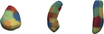
Parcellation of the three structures using spectral clustering. The average segment size is 50 mm ² . Amygdala: 15 segments, hippocampus: 29 segments, ERC: 10 segments.

3.2. Statistical analysis via the morphometric changepoint model

We analyze the shape markers with a model describing a change in a linear atrophy rate happening some number, Δ, of years before the estimated age of clinical onset, forming a morphometry changepoint before clinical symptom onset time. We assume linear models for the absolute volume and atrophy as a function of age, with a change of slope at changepoint. In mathematical terms, if a is the age and t is the time of clinical onset, the model takes the form a→ α+ βa before morphometry changepoint, a ≤ t − Δ, and becomes a→ α+ βa+ β′(a− t− Δ) subsequent to the changepoint. For the controls, the onset time of clinical symptom is (if it ever occurs) beyond the end of the study and the associated model retains the same linear rate over the considered time period. This model, which is depicted in Fig. 2, can be related to the sigmoidal model introduced in Jack et al. (2013), in which biomarkers smoothly transition from a low-abnormality plateau to a high-abnormality one in an S-shaped curve. Under Jack's model, almost no patient from our dataset would have reached the high-abnormality plateau at scan times, and we therefore expect to observe them while they are either in the low-abnormality plateau, or in the transition phase, which justifies using a model with two regimes only. Note that our model does not include a second changepoint at clinical onset time. Since there is no reason for structure atrophy to switch regime at the very time the disease becomes detectable by clinical tests, we do not expect any direct causal effect of clinical onset on the morphometry. Of course, the two-piece model we consider allows for both structural changepoint and clinical onset time to coincide (i.e., Δ = 0).

Fig. 2.

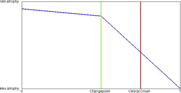
Schematic illustration of the changepoint model. The atrophy regime changes at changepoint, several years before clinical onset.

The analysis includes gender and log-intracranial volumes as covariates, and uses a random effect model to account for inter-subject versus intra-subject shape variation (see details in Appendix A). We test for the null hypothesis of constant-rate atrophy in the whole cohort versus the alternate changepoint model and compute statistics at each subregion of the segmented template surface, as delineated in Fig. 1, returning p-values corrected for multiple comparisons using permutation testing (Nichols and Hayasaka, 2003). Permutation testing applied to multiple hypotheses associated with subregions of the structures provides a unique p-value for rejecting the compound null that all individual nulls are true, i.e., that the onset model applies to none of the regions in the segmented structure. Assuming that the compound null is rejected, the method also provides an estimate of the set of significant regions, which is conservative in the sense that the probability of making a single false detection is small (5% in our results). This is usually referred to as controlling the family-wise error rate (FWER) at the 5% level. In addition to the permutation testing, we used a resampling method (bootstrap) to assess the accuracy of the estimated onset time, allowing us to provide an indication of the standard deviation of our estimated changepoint. More details on our implementation of permutation testing and bootstrap validation are provided in Appendix A.

4. Results

The curves in Fig. 3 show the log-likelihood calculation for the segment morphometry markers as a function of the parameter Δ (the plotted log-likelihoods are obtained by maximizing over every model parameter except Δ). The changepoint estimator is the maximizer of this curve. The top rows in Fig. 3 show the left and right sides of the amygdala, the middle row shows those of the hippocampus, and the bottom row shows those of the ERC. The curves for the amygdala and the hippocampus are highest at around 2 years before clinical onset, while the likelihood for the ERC is largest at around 10 years before onset. The bootstrap-estimated standard deviations of these sample estimates lie between 1 and 3 years as reported in Table 2.

Fig. 3.

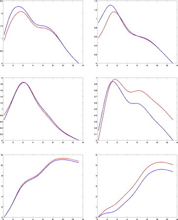
Log-likelihood as a function of changepoint for the amygdala (top), the hippocampus (middle) and the entorhinal cortex (bottom), with left structure on the leftcolumn and right on the right one. The left hippocampus is not significant and is only provided here for completeness. Likelihoods are averaged over all segments constituting the surface. The red curve is the likelihood obtained on the original sample, andthe blue one is averaged over bootstrap resampling. Both curves are offset so that their minimum value is zero, to simplify visualization.

Table 2.

Differences in estimated onset of morphometric change in relationship to symptom onset for the amygdala, entorhinal cortex and hippocampus. The p-value, corrected for multiple comparisons, is obtained for each structure via permutation tests, as described in the Methods section (the lowest detectable p-value is 10⁻⁴). The reported onset time for each structure is estimated via bootstrap (the standard deviation between parentheses measuring its accuracy).

Side		Amygdala volume	Amygdala segment	Hippocampus volume	Hippocampus segment	ERC volume	ERC segment
Left	p-Value	0.003	0.006	0.017	0.13	0.0001	0.0001
	Avg. Δ (std.)	2.8 (2.3)	2.5 (1.4)	3.1 (1.9)	2.6 (1.0)	7.5 (2.5)	8.6 (1.5)
Right	p-Value	0.006	0.0015	0.27	0.024	0.0007	0.004
	Avg. Δ (std.)	2.5 (3.3)	2.7 (1.9)	4.0 (3.8)	3.6 (1.4)	9.9 (3.0)	8.5 (2.8)

Table 2 also provides the p-values associated with the changepoint model for the ERC, amygdala, and hippocampus. The segment-averaged measures in the right hemisphere show significant differences between the groups as follows: the ERC is significant (p= 0.004) with a changepoint at around 8.5 years (±2.8). The hippocampus is marginally significantly different (p= 0.024), with a changepoint estimated at 3.6 (±1.4) years prior to symptom onset, and the amygdala is strongly significant (p= 0.0015), with a changepoint at 2.7 (±1.9) years before onset. For the left hemisphere, the significant differences are as follows: (1) the entorhinal cortex demonstrates a significant difference (p< 0.0001) 8.6 (±1.5) years prior to symptom onset, and (2) the amygdala shows significant differences (p= 0.006) 2.5 (±1.4) years prior to symptom onset. The left hippocampus shows no significance. The volume measures are significant for the amygdala (left: p= 0.003, right: p= 0.006), significant on the left side (p= 0.017) for the hippocampus, and not significant on the right (p= 0.27). Volume is significant for the ERC (left: p< 0.0001, right: p= 0.0007).

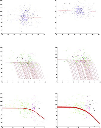
Figs. 4–6 provide predicted atrophy curves with changepoint estimated from our model for all diseased subjects. The morphometric measure is the amount of surface area variation relative to the templates, and is expressed in percentages, with 100% meaning no difference from the template. To simplify visualization, all curves are plotted using the same covariate values (gender and intracranial volume) for all subjects, taken equal to their population averages. Since there is one such curve per segment, they are also averaged over all segments in each structure. The evolution starts with a nearly horizontal line, which coincides with the one associated with controls, then changes to a steeper slope at changepoint. The smoothness of the transition is due to averaging, since changepoints are not identical for each segment. The middle row in Figs. 4–6 plots these curves against subject age, while the bottom row provides the same curves shifted by clinical onset age, which enables comparison (the slopes are the same in both cases, even though the unshifted curves appear steeper; this is due to the rescaling of the horizontal axis for shifted curves). These plots also visualize the actual morphometric measure (still averaged over segments) for all cognitively impaired cases, represented as dots colored according to whether the scan is taken before changepoint, between changepoint and clinical onset, or after clinical onset. Since the estimated changepoint for the ERC is around 9 years before clinical symptom onset, only a few scans of preclinical cases predate it (the pre-changepoint line is primarily estimated based on control subjects). The transition appears more clearly with the amygdala for which the two regimes are observed, with a quasi-horizontal line followed by a decreasing one after changepoint. The same goes for the right hippocampus. The top row of Figs. 4–6 represents the controls, together with the regression line that is associated with them (identical to the regime before changepoint).

Fig. 4.

Amygdala: left and right; blue: controls; green: before changepoint; magenta: before clinical onset; black: after clinical onset. The y -axis shows the surface area percentage around each vertex expressed relative to original template coordinates averaged over all segments. Top row: controls with their associated regression line. Middle row: cognitively impaired subjects. Third row: cognitively impaired subjects with time axis shifted by clinical onset. All values are corrected for random effects.

Fig. 5.

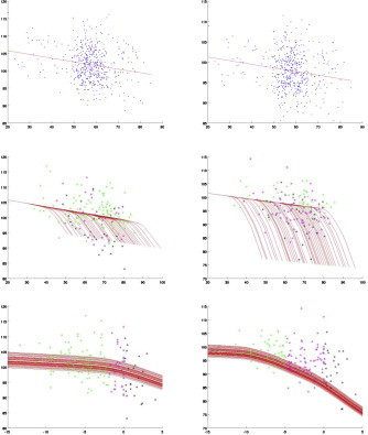
Hippocampus: left and right; blue: controls; green: before changepoint; magenta: before clinical onset; black: after clinical onset. The y -axis shows the surface area percentage around each vertex expressed relative to original template coordinates averaged over all segments. Top row: controls with their associated regression line. Middle row: cognitively impaired subjects. Third row: cognitively impaired subjects with time axis shifted by clinical onset. All values are corrected for random effects.

Fig. 6.

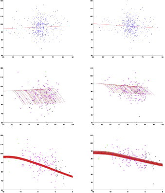
ERC: left and right; blue: controls; green: before changepoint; magenta: before clinical onset; black: after clinical onset. The y -axis shows the surface area percentage around each vertex expressed relative to original template coordinates averaged over all segments. Top row: controls with their associated regression line. Middle row: cognitively impaired subjects. Third row: cognitively impaired subjects with time axis shifted by clinical onset. All values are corrected for random effects.

Fig. 7 maps the value of the surface atrophy rate (per year) that was detected on segments for which the onset model was found significant at 5% FWER. These atrophy rates are defined as 100(exp(β) − 1) before changepoint and 100(exp(β+ β′) − 1) after changepoint (see details in Appendix A). Table 3 provides the numerical values of the after-changepoint rates for each structure and side, with β and β′ replaced by their average values over all segments. In this table, we have applied the changepoint model to a reduced cohort containing subjects with three scans or more (81 controls and 30 cognitively impaired), to improve accuracy. For the left ERC, one finds 2.4% after changepoint and 0.1% before. On the right side, the rate is 1.6% after and 0.2% before. For the amygdala, the left side gives 3.6% after and 0.1% before, and the right side is 4.6% after and 0.2% before. Finally, the left hippocampus shows a 1.2% atrophy rate after changepoint, and a 0.2% rate before. The right side gives 2.7% after and 0.2% before. The onset model, on the reduced cohort, was found significant in all cases. Table 3 also provides atrophy rates in terms of global volume, for which only the right hippocampus was found non-significant. Note that surface atrophy rates and volume atrophy rates are not directly comparable, although one can expect the former to be roughly 2/3 of the latter, which is consistent with what we observe in our results.

Fig. 7.

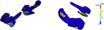
Significant pattern of atrophy rate change. Left panel: seen from patient left side; right panel: seen from patient right side. The structures visualized in the left panel are the amygdala, hippocampus and ERC from left to right, and their order is reversed on the right panel. Color represents rate change coefficient, in percentages, after changepoint when significant. Deep blue color (0%) indicates non-significance for the corrected p -value.

Table 3.

Estimated atrophy rates per year, estimated over subjects with three scans or more (81 controls, 30 MCI/AD) for total volume and segments (averaged over all segments) on each structure (NS: non-significant).

Side		Amygdala volume	Amygdala segments	Hippocampus volume	Hippocampus segments	ERC volume	ERC segments
Left	Before	−0.3%	−0.1%	−0.35%	−0.2%	−0.3%	−0.1%
	After	−4.2%	−3.6%	−1.6%	−1.2%	−3.0%	−2.4%
Right	Before	−0.45%	−0.2%	−0.4%	−0.2%	−0.45%	−0.2%
	After	−5.0%	−4.6%	−1.7% (NS)	−2.7%	−2.7%	−1.6%

5. Discussion

The high-dimensional morphometry model indicates that, during preclinical AD, changes in the shape of the entorhinal cortex precede those in the hippocampus and the amygdala. In general, the high-dimensional diffeomorphometry-based markers are more significant than the volume markers in signaling the changepoint time. This is the first time to our knowledge that diffeomorphometry has been coupled to changepoint models to examine differences in atrophy rates among brain structures preceding clinical symptom onset.

The finding of localized ERC change preceding the changepoint in the other two temporal lobe structures is consistent with previous MRI reports of ERC volume change during MCI. For example, a differential rate of change in the ERC, compared to the hippocampus, has previously been reported among individuals with MCI who subsequently progressed to AD dementia (Du et al., 2001, 2006; Dickerson et al., 2001; Jagust et al., 2006; Du et al., 2006; Jack et al., 2010). The finding of significant differences in morphometry change in the amygdala is consistent with morphometry reported in symptomatic AD, such as the volume (Poulin et al., 2011) and shape analysis (Cavedo et al., 2011; Qiu et al., 2009b). Alterations in the entorhinal cortex and hippocampus are consistent with changes in memory performance reported during preclinical AD. Psychiatric symptomatology (such as apathy and irritability) have been reported in MCI cases that subsequently progressed to dementia, and it has been suggested that this may, in part, result from pathological changes in the amygdala. Further study is needed to directly link the ordering of these clinical features with respect to one another, and to the brain changes reported here.

Evidence of morphometry changes occurring approximately 10 years prior to symptom onset is also consistent with current hypotheses about the long prodromal phase of AD (Jack et al., 2013). This study adds additional evidence to support the hypothesis that there are significant changes in the brain many years before symptom onset. It is hypothesized that early therapeutic intervention will have the best prospect for modifying disease progression and confer the greatest benefit to patients in the early stages of AD. Understanding the order in which changes in the brain occur during preclinical AD may therefore assist in the design of intervention trials aimed at slowing the evolution of the disease.

It is important to acknowledge the challenges of estimating age of symptom onset. While we used a semi-standardized instrument administered to both the subject and an informant, with specific targeted questions to assess onset of symptoms, known as the Clinical Dementia Rating Scale (Morris et al., 1993), the determination was ultimately based on the judgment of skilled clinicians. It should be noted, however, that we have recently published data on CSF changes in relation to symptom onset in this cohort (Moghekar et al., 2013), suggesting that this measure is biologically meaningful.

Several issues must be entertained in considering the validity of our statistical analyses. First, the number of available scans can vary among subjects (i.e., there are missing data) and our p-value computation requires the assumption that this censoring is independent of the group variables. This is a reasonable assumption, since most subjects were not cognitively impaired when the scans were taken. This assumption is partially confirmed by the fact that there is no significant difference between the numbers of scans per subject in the two groups (p= 0.063), although this p-value is small enough to be a concern. If we limit the analysis to subjects that had two scans or more (resp. three scans or more), however, this p-value becomes p= 0.28 (resp. p= 0.59), and the results that are obtained in these cases show very few differences compared to the ones obtained for the main study. These results are included in Table 4 for comparison with Table 2.

Table 4.

Differences in estimated onset of morphometric change in relationship with symptom onset for the amygdala, entorhinal cortex and hippocampus, for the cohort reduced to patients with two scans or more (136 controls and 46 impaired) and with three scans or more (81 controls and 30 impaired). The results are very similar to those obtained with the complete cohort in Table 2.

Side			Amygdala volume	Amygdala segments	Hippocampus volume	Hippocampus segments	ERC volume	ERC segments
Left	p-Value	≥ 2	0.002	0.0009	0.024	0.15	0.0001	0.0005
		≥ 3	0.0001	0.0003	0.015	0.02	0.0005	0.0001
	Avg. Δ (std.)	≥ 2	3.1 (2.3)	2.4 (1.4)	2.8 (1.6)	2.4 (1.1)	7.4 (3.2)	8.5 (2.0)
		≥ 3	2.3 (2.1)	2.5 (1.2)	2.2 (1.5)	2.4 (1.1)	5.5 (3.5)	6.8 (2.3)
Right	p-Value	≥ 2	0.006	0.0015	0.25	0.07	0.002	0.013
		≥ 3	0.0005	0.007	0.18	0.003	0.005	0.01
	Avg. Δ (std.)	≥ 2	2.8 (3.6)	3.4 (2.1)	3.0 (3.9)	2.8 (1.3)	9.9 (3.2)	8.0 (3.2)
		≥ 3	2.2 (3.5)	3.1 (2.0)	3.2 (4.6)	2.2 (1.2)	9.7 (3.2)	7.9 (3.2)

The second issue is whether the changepoint that is observed is actually related to the disease, or whether it may be confounded with a normal changepoint occurring also in controls (so that our significant p-values would reflect the inadequacy of the model for controls, rather than the existence of a disease-related changepoint). To examine this possibility, we extended our analysis to include a “normal changepoint”, obtained by analyzing the control population, and used this changepoint to define an additional covariate in our previous analysis. Doing so did not impact our conclusion, yielding very minor changes in the obtained p-values (data not shown).

It should be acknowledged that the boundaries between normal aging and the earliest symptomatic phase of AD are difficult to define. Studies in both animal models and humans demonstrate that there are significant cognitive and neurobiological changes with aging, in the absence of disease (see Samson and Barnes, 2013 for a review). Additionally, AD pathophysiological processes are evident in a subset of older adults who are cognitively normal (Sperling et al., 2011). Studies, such as ours, in which cognitively normal individuals are followed for many years (with some remaining normal and some developing MCI and AD dementia) are one of the best ways currently available of disentangling changes related to aging from those that are a harbinger of disease.

Appendix A

A1. Statistical details

A1.1. Shape variables at each vertex

Denote by a_kj the age of subject k at their jth scan and by t_k the time of clinical onset of the disease for the same subject. This time is only defined for subjects in the MCI/AD group, and we let g_k be the associated indicator variable, equal to one for subjects in this group and to zero for controls. We also let c_k denote the intracranial volume and d_k the gender of subject k (zero for males, one for females). For the jth scan of subject k, shape markers are computed at each vertex coordinate and averaged over each template segment (shown in Fig. 1); they are denoted by $y_{kj}^q$, where q is the segment index. In the case of volume, then the log-volume is used as a one-dimensional shape marker.

A1.2. Changepoint onset model

We now describe the changepoint model introducing the explicit role of the ordering parameter Δ in the atrophy model signaling in years the changepoint time preceding clinical symptom time. For this we use the changepoint model with linear atrophy turning on Δ years before clinical symptom

$$\begin{gathered} y_{kj}^q={\alpha }_q+{\beta }_q{a}_{kj}+{\beta }_q^{\text{'}}{g}_k\left(a_{kj}-t_k+{\text{Δ}}^q\right)H\left(a_{kj}-t_k+{\text{Δ}}^q\right) \\ +{\gamma }_q{c}_k+{\delta }_q{d}_k+{ϵ}_{kj}^q \end{gathered}$$

in which H is the Heaviside function, such that H(t)=1 if t> 0 and H(t) = 0 otherwise. The noise, ${\epsilon }_{kj}^q$, includes random effects and decomposes as

$${\epsilon }_{kj}^q={\eta }_k^q+{\zeta }_{kj}^q$$

in which all variables η and ζ with distinct indices are assumed to be independent, ${\eta }_k^q\sim N(0,{\rho }_q^2)$ and ${\zeta }_{kj}^q\sim N(0,{\sigma }_q^2)$. The model parameters are ${\alpha }_q,{\beta }_q,{\beta }_q^{\prime },{\text{Δ}}^q,{\sigma }_q^2$ and ${\rho }_q^2$ (q indexing the shape coordinates). They are estimated by maximum likelihood.

Via the transition function, the model implies a first-order changepoint from atrophy rate β_q to ${\beta }_q+{\beta }_q^{\text{'}}$ at age a = t_k − Δ^q, i.e., Δ^q years before cognitive onset. Controls, for which g_k = 0, remain in the first regime over the observation time. Recall that the vertex-indexed shape variables describe the relative value of surface area around a given point at logarithmic scale, where the template is the reference. As a consequence, our model can be interpreted as

• Before changepoint:

(local surface area) = (template local surface area) × (correction based on covariates) × exp(β_q⋅ age)

• After changepoint:

(local surface area) = (template local surface area) × (correction based on covariates) × ((β_q+ β^'_q) ⋅ age − β_q ⋅ (age at changepoint))

In other words, ${\beta }_q^{\text{'}}\ne 0$ implies a multiplicative factor of $\exp \left({\beta }_q^{\text{'}}\right)$ per year in surface area post changepoint. This is atrophy as soon as ${\beta }_q^{\text{'}}$ is negative, as found in our results.

We can interpret t_k− Δ^q as a structural, or anatomical, phenotype onset time. In the following, we will test the null hypothesis ${\beta }_q^{\text{'}}=0$, which corresponds to the disease having no effect on the shape coordinate q. When this hypothesis is rejected with significant p-value (corrected for multiple comparisons), we can compute a consensus estimator, defined as the average of all estimated Δ^q over coordinates q.

A1.3. Estimation procedure

The following computation is made independently for each shape coordinate q that we temporarily drop from the notation. We compute a maximum likelihood estimator for fixed values of Δ, taken from a discrete interval over the timeframe of interest, which is −2 to 13 years, with half-year increments. The computation with fixed Δ uses the EM algorithm (Dempster et al., 1977) to estimate the remaining parameters, treating the random effects η_k as hidden variables. The EM algorithm alternates, until stabilization, an E-step, in which the log-likelihood is averaged using the conditional distribution given observed variables, and an M-step, in which this conditionally averaged likelihood is maximized with respect to the model parameters. More details follow.

E-step: Since we are working with fixed Δ, introduce for convenience the variable

$$u_{kj}=g_k\left(a_{kj}-t_k+\text{Δ}\right)H\left(a_{kj}-t_k+\text{Δ}\right)$$

so that the model can be written as

$$y_{kj}=\alpha +\beta a_{kj}+{\beta }^{\prime }{u}_{kj}+\gamma c_k+d_k+{\eta }_k+{\zeta }_{kj}$$

(recall that several variables, including u_kj, depend on the shape coordinate, q, even though this dependency is not made explicit). The joint log-likelihood is then given by

$$\begin{gathered} \ell =-\frac{1}{2{\sigma }^2}\sum _{k=1}^n\sum _{j=1}^{n_k}{\left(y_{kj}-\alpha -\beta a_{kj}-{\beta }^{\text{'}}{u}_{kj}-\gamma c_k-\delta d_k-{\eta }_k\right)}^2 \\ -\frac{1}{2{\rho }^2}\sum _{k=1}^n{\eta }_k^2–\frac{N}{2}\log {\sigma }^2-\frac{n}{2}\log {\rho }^2 \end{gathered}$$

where n is the number of subjects, n_k the number of scans for subject k and N is the total number of scans. Let r_kj denote the residual (y_kj − α − βa_kj − β^′u_kj − γc_k − δd_k − η_k). Conditional to observed variables y, a, u, c, and d, the hidden variable η_k follows a Gaussian distribution with mean and variance

$$m_k=\frac{{\rho }^2}{{\sigma }^2+n_k{\rho }^2}{\left(\sum _{j=1}^{n_k}{r}_{kj}\right)}^2,{\tau }_k^2=\frac{{\rho }^2{\sigma }^2}{n_k{\rho }^2+{\sigma }^2}.$$

From this, it follows that the conditional likelihood is, up to an additive constant:

$$\begin{gathered} {\ell }_{\text{cond}}=-\frac{1}{2{\sigma }^2}\sum _{k=1}^n\sum _{j=1}^{n_k}{\left(y_{kj}-m_k-\alpha -\beta a_{kj}-{\beta }^{\text{'}}{u}_{kj}-\gamma c_k-\delta d_k\right)}^2 \\ -\frac{1}{2{\sigma }^2}\sum _{k=1}^n{n}_k{\tau }_k^2-\frac{1}{2{\rho }^2}\sum _{k=1}^n\left({\tau }_k^2+m_k^2\right)-\frac{n}{2}\log {\rho }^2-\frac{N}{2}\log {\sigma }^2 \end{gathered}$$

M-step: This likelihood is optimized with respect to the parameters in the M-step: α, β, β^′, γ, δ' are updated via linear regression of the shape variables y_kj − m_k against the other variables, which is obtained via standard least squares. The parameters σ² and ρ² are then derived via

$$\begin{gathered} {\sigma }^2=\frac{1}{N}\sum _{k=1}^n\sum _{j=1}^{n_k}{\left(y_{kj}-m_k-\alpha -\beta a_{kj}-{\beta }^{\text{'}}{u}_{kj}-\gamma c_k-\delta d_k\right)}^2 \\ +\frac{1}{N}\sum _{k=1}^n{n}_k{\tau }_k^2 \end{gathered}$$

and

$${\rho }^2=\frac{1}{n}\sum _{k=1}^n({\tau }_k^2+m_k^2).$$

These values are then plugged back into the E-step for another iteration of the EM algorithm, which is run until stabilization.

At the end of the algorithm, the likelihood of the observed variables is obtained by integrating with respect to the random effects. It is, still up to constant additive factors, and using the same notation for m_k and ${\tau }_k^2$, given by the following expression: $L=-\frac{1}{2{\sigma }^2}\sum _{k=1}^n\left({\left(\sum _{j=1}^{n_k}{r}_{kj}\right)}^2-m_k^2\right)-\frac{N}{2}\log {\sigma }^2-\frac{n}{2}\log {\rho }^2+\frac{1}{2}\sum _{k=1}^n\log {\tau }_k^2$. Remembering that we were working with fixed shape coordinate q and fixed Δ, this likelihood is actually a function of both q and Δ. Denote it by L^q(Δ). This likelihood is then optimized in Δ by computing it over a finite number of values, yielding an optimal Δ^q, associated with parameters  $\left({\alpha }_q,{\beta }_q,{\beta }_q^{\text{'}},{\gamma }_q,{\delta }_q,{\sigma }_q,{\rho }_q\right)$. The optimal likelihood, L^q(Δ^q), will be used below to assess model significance.

Note that the optimization under the null hypothesis (${\beta }_q^{\text{'}}=0)$ follows exactly the same approach, using the EM algorithm, except that, since the model under the null does not depend on Δ, there is no final optimization loop with respect to this parameter. This computation returns a likelihood under the null, that we will denote by $L_0^q$.

A1.4. Tests for significance

Our tests are based on the likelihood ratio statistic, which is computed independently for each shape coordinate, q, and is given, with our previous notation, by

$$S_q=L^q\left({\text{Δ}}^q\right)-L_0^q.$$

A global statistic is then defined by $S_{\text{max}}=\underset{q}{\max }{S}_q$. To compute p-values, we use permutation tests, randomizing the model residuals, which are defined by

$${\lambda }_{kj}^q=y_{kj}^q-{\alpha }_q-{\beta }_q{a}_{kj}-\gamma c_k-d_k$$

where the parameters are estimated under the null hypothesis.

Permutations operate over subjects, i.e., on the index k, so that scans that were associated to the same subject remain together. Let ${\lambda }_{kj}^{q,\pi }$. Denote the residuals after applying a permutation π. We apply the estimation scheme developed in the previous section after replacing $y_{kj}^q$ by ${\lambda }_{kj}^{q,\pi }$, computing new likelihood ratios $S_q^{\pi }$, and global statistic $S_{\text{max}}^{\pi }$. We repeat this for a large number, say M, of random permutations, and compare the obtained statistics to the one associated to the original ${\lambda }_{kj}^q$, i.e., $S_{\text{max}}^{\text{id}}$ for π= identity. If ν is the number of permutations π for which the value of $S_{\text{max}}^{\pi }$ excess $S_{\text{max}}^{\text{id}}$, the associated p-value is given by

$$p=\frac{\nu +1}{M+1}.$$

We used M = 10,000 in our experiments, making p = 0.0001 the smallest detectable p-value.

Variables q for which $S_q^{\text{id}}$ is found larger that the 95th percentile of the values of $S_{\text{max}}^{\pi }$ that were observed via permutations are considered as significantly affected by group difference. These variables are detected at a 5% family-wise error rate (FWER), which means that the probability of making one or more false detections among them is less than 5%.

As a final remark in this section, we mention that, since one of the issues of the EM algorithm is that its solution may depend on the initialization, we always initialize the estimation scheme for the alternate hypothesis with the one found with the null hypothesis. This ensures the positivity of the log–likelihood ratio statistics.

A1.5. Accuracy assessment via bootstrap

To evaluate the accuracy of the changepoint estimate, we performed a resampling procedure (bootstrap). Each resample step draws subjects from the original dataset with replacement, in order to obtain a new dataset with the same size. A new summary onset time, say Δ^*, is estimated from this dataset. By repeating this procedure a large number of times, one obtains bootstrap estimates of the mean and standard deviation of the estimator. This measures the accuracy of our results, and should not be confused with a population standard deviation of the onset time, since we estimate only one Δ for the whole cohort and cannot assess its variability across subjects (the small number of scans per subject make the computation of individual changepoints impossible).

References

- Apostolova L.G., Mosconi L., Thompson P.M., Green A.E., Hwang K.S., Ramirez A., Mistur R., Tsui W.H., de Leon M.J. Subregional hippocampal atrophy predicts Alzheimer's dementia in the cognitively normal. Neurobiology of Aging. 2010;31:1077–1088. doi: 10.1016/j.neurobiolaging.2008.08.008. 18814937 [DOI] [PMC free article] [PubMed] [Google Scholar]
- Arnold S.E., Hyman B.T., Flory J., Damasio A.R., van Hoesen G.W. The topographical and neuroanatomical distribution of neurofibrillary tangles and neuritic plaques in the cerebral cortex of patients with Alzheimer's disease. Cerebral Cortex (New York, N.Y.: 1991) 1991;1:103–116. doi: 10.1093/cercor/1.1.103. 1822725 [DOI] [PubMed] [Google Scholar]
- Arriagada P.V., Growdon J.H., Hedley-Whyte E.T., Hyman B.T. Neurofibrillary tangles but not senile plaques parallel duration and severity of Alzheimer's disease. Neurology. 1992;42:631–639. doi: 10.1212/wnl.42.3.631. 1549228 [DOI] [PubMed] [Google Scholar]
- Ashburner J., Csernansky J.G., Davatzikos C., Fox N.C., Frisoni G.B., Thompson P.M. Computer-assisted imaging to assess brain structure in healthy and diseased brains. Lancet Neurology. 2003;2:79–88. doi: 10.1016/s1474-4422(03)00304-1. 12849264 [DOI] [PubMed] [Google Scholar]
- Atiya M., Hyman B.T., Albert M.S., Killiany R. Structural magnetic resonance imaging in established and prodromal Alzheimer disease: a review. Alzheimer Disease and Associated Disorders. 2003;17:177–195. doi: 10.1097/00002093-200307000-00010. 14512832 [DOI] [PubMed] [Google Scholar]
- Braak H., Braak E. Neuropathological staging of Alzheimer-related changes. Acta Neuropathologica. 1991;82:239–259. doi: 10.1007/BF00308809. 1759558 [DOI] [PubMed] [Google Scholar]
- Carlson N.E., Moore M.M., Dame A., Howieson D., Silbert L.C., Quinn J.F., Kaye J.A. Trajectories of brain loss in aging and the development of cognitive impairment. Neurology. 2008;70:828–833. doi: 10.1212/01.wnl.0000280577.43413.d9. 18046010 [DOI] [PubMed] [Google Scholar]
- Cavedo E., Boccardi M., Ganzola R., Canu E., Beltramello A., Caltagirone C., Thompson P.M., Frisoni G.B. Local amygdala structural differences with 3T MRI in patients with Alzheimer disease. Neurology. 2011;76:727–733. doi: 10.1212/WNL.0b013e31820d62d9. 21339500 [DOI] [PMC free article] [PubMed] [Google Scholar]
- Chiang M.C., Avedissian C., Barysheva M., Toga A.W., Mcmahon K.L., de Zubicaray G.I., Wright M.J., Thompson P.M. Extending genetic linkage analysis to diffusion tensor images to map single gene effects on brain fiber architecture. Medical Image Computing and Computer-Assisted Intervention: MICCAI ... International Conference on Medical Image Computing and Computer-Assisted Intervention. 2009;12:506–513. doi: 10.1007/978-3-642-04271-3_62. 20426150 [DOI] [PubMed] [Google Scholar]
- Csernansky J.C., Joshi S., Wang L., Gado M., Miller J.P., Grenander U., Miller M.I. Hippocampal morphometry in schizophrenia by high dimensional brain mapping. Proceedings of the National Academy of Sciences of the United States of America. 1998;95:11406–11411. doi: 10.1073/pnas.95.19.11406. 9736749 [DOI] [PMC free article] [PubMed] [Google Scholar]
- Csernansky J.G., Wang L., Joshi S., Miller J.P., Gado M., Kido D., Mckeel D., Morris J.C., Miller M.I. Early DAT is distinguished from aging by high-dimensional mapping of the hippocampus. Dementia of the Alzheimer type. Neurology. 2000;55:1636–1643. doi: 10.1212/wnl.55.11.1636. 11113216 [DOI] [PubMed] [Google Scholar]
- Csernansky J.G., Wang L., Swank J., Miller J.P., Gado M., Mckeel D., Miller M.I., Morris J.C. Preclinical detection of Alzheimer's disease: hippocampal shape and volume predict dementia onset in the elderly. Neuroimage. 2005;25:783–792. doi: 10.1016/j.neuroimage.2004.12.036. 15808979 [DOI] [PubMed] [Google Scholar]
- Cummings J.L., Mega M., Gray K., Rosenberg-Thompson S., Carusi D.A., Gornbein J. The neuropsychiatric inventory: comprehensive assessment of psychopathology in dementia. Neurology. 1994;44:2308–2314. doi: 10.1212/wnl.44.12.2308. 7991117 [DOI] [PubMed] [Google Scholar]
- Dempster A., Laird N., Rubin D. Maximum likelihood from incomplete data via the EM algorithm. Journal of the Royal Statistical Society. Series B (Methodological) 1977;39:1–38. [Google Scholar]
- den Heijer T., Geerlings M.I., Hoebeek F.E., Hofman A., Koudstaal P.J., Breteler M.M. Use of hippocampal and amygdalar volumes on magnetic resonance imaging to predict dementia in cognitively intact elderly people. Archives of General Psychiatry. 2006;63:57–62. doi: 10.1001/archpsyc.63.1.57. 16389197 [DOI] [PubMed] [Google Scholar]
- Dickerson B.C., Goncharova I., Sullivan M.P., Forchetti C., Wilson R.S., Bennett D.A., Beckett L.A., Detoledo-Morrell L. MRI-derived entorhinal and hippocampal atrophy in incipient and very mild Alzheimer's disease. Neurobiology of Aging. 2001;22:747–754. doi: 10.1016/s0197-4580(01)00271-8. 11705634 [DOI] [PubMed] [Google Scholar]
- Du A.T., Jahng G.H., Hayasaka S., Kramer J.H., Rosen H.J., Gorno-Tempini M.L., Rankin K.P., Miller B.L., Weiner M.W., Schuff N. Hypoperfusion in frontotemporal dementia and Alzheimer disease by arterial spin labeling MRI. Neurology. 2006;67:1215–1220. doi: 10.1212/01.wnl.0000238163.71349.78. 17030755 [DOI] [PMC free article] [PubMed] [Google Scholar]
- Du A.T., Schuff N., Amend D., Laakso M.P., Hsu Y.Y., Jagust W.J., Yaffe K., Kramer J.H., Reed B., Norman D., Chui H.C., Weiner M.W. Magnetic resonance imaging of the entorhinal cortex and hippocampus in mild cognitive impairment and Alzheimer's disease. Journal of Neurology, Neurosurgery, and Psychiatry. 2001;71:441–447. doi: 10.1136/jnnp.71.4.441. 11561025 [DOI] [PMC free article] [PubMed] [Google Scholar]
- Herzog A.G., Kemper T.L. Amygdaloid changes in aging and dementia. Archives of Neurology. 1980;37:625–629. doi: 10.1001/archneur.1980.00500590049006. 7425886 [DOI] [PubMed] [Google Scholar]
- Hughes C.P., Berg L., Danziger W.L., Coben L.A., Martin R.L. A new clinical scale for the staging of dementia. British Journal of Psychiatry: the Journal of Mental Science. 1982;140:566–572. doi: 10.1192/bjp.140.6.566. 7104545 [DOI] [PubMed] [Google Scholar]
- Jack C.R., Knopman D.S., Jagust W.J., Petersen R.C., Weiner M.W., Aisen P.S., Shaw L.M., Vemuri P., Wiste H.J., Weigand S.D., Lesnick T.G., Pankratz V.S., Donohue M.C., Trojanowski J.Q. Tracking pathophysiological processes in Alzheimer's disease: an updated hypothetical model of dynamic biomarkers. Lancet Neurology. 2013;12:207–216. doi: 10.1016/S1474-4422(12)70291-0. 23332364 [DOI] [PMC free article] [PubMed] [Google Scholar]
- Jack C.R., Knopman D.S., Jagust W.J., Shaw L.M., Aisen P.S., Weiner M.W., Petersen R.C., Trojanowski J.Q. Hypothetical model of dynamic biomarkers of the Alzheimer's pathological cascade. Lancet Neurology. 2010;9:119–128. doi: 10.1016/S1474-4422(09)70299-6. 20083042 [DOI] [PMC free article] [PubMed] [Google Scholar]
- Jack C.R., Shiung M.M., Gunter J.L., O'Brien P.C., Weigand S.D., Knopman D.S., Boeve B.F., Ivnik R.J., Smith G.E., Cha R.H., Tangalos E.G., Petersen R.C. Comparison of different MRI brain atrophy rate measures with clinical disease progression in AD. Neurology. 2004;62:591–600. doi: 10.1212/01.wnl.0000110315.26026.ef. 14981176 [DOI] [PMC free article] [PubMed] [Google Scholar]
- Jagust W., Gitcho A., Sun F., Kuczynski B., Mungas D., Haan M. Brain imaging evidence of preclinical Alzheimer's disease in normal aging. Annals of Neurology. 2006;59:673–681. doi: 10.1002/ana.20799. 16470518 [DOI] [PubMed] [Google Scholar]
- Kantarci K., Jack C.R. Neuroimaging in Alzheimer disease: an evidence-based review. Neuroimaging Clinics of North America. 2003;13:197–209. doi: 10.1016/s1052-5149(03)00025-x. 13677801 [DOI] [PubMed] [Google Scholar]
- Ma J., Miller M.I., Younes L. A Bayesian generative model for surface template estimation. International Journal of Biomedical Imaging. 2010 doi: 10.1155/2010/974957. [DOI] [PMC free article] [PubMed] [Google Scholar]
- Miller M., Younes L., Ratnanather J., Brown T., Trinh H., Postell E., Lee D., Wang M.-C., Mori S., O'Brien R. The diffeomorphometry of temporal lobe structures in preclinical Alzheimer's disease. NeuroImage: Clinical. 2013;3:352–360. doi: 10.1016/j.nicl.2013.09.001. 24363990 [DOI] [PMC free article] [PubMed] [Google Scholar]
- Miller, M.I., Trouve, A., Younes, L., Diffeomorphometry and geodesic positioning systems for human anatomy. Technology 20140126 (2013): 1–9 [DOI] [PMC free article] [PubMed]
- Munn M.A., Alexopoulos J., Nishino T., Babb C.M., Flake L.A., Singer T., Ratnanather J.T., Huang H., Todd R.D., Miller M.I., Botteron K.N. Amygdala volume analysis in female twins with major depression. Biological Psychiatry. 2007;62:415–422. doi: 10.1016/j.biopsych.2006.11.031. 17511971 [DOI] [PMC free article] [PubMed] [Google Scholar]
- Morris J.C. The clinical dementia rating (CDR): current version and scoring rules. Neurology. 1993;43:2412–2414. doi: 10.1212/wnl.43.11.2412-a. 8232972 [DOI] [PubMed] [Google Scholar]
- Nichols T., Hayasaka S. Controlling the familywise error rate in functional neuroimaging: a comparative review. Statistical Methods in Medical Research. 2003;12:419–446. doi: 10.1191/0962280203sm341ra. 14599004 [DOI] [PubMed] [Google Scholar]
- Poulin S.P., Dautoff R., Morris J.C., Barrett L.F., Dickerson B.C. Amygdala atrophy is prominent in early Alzheimer's disease and relates to symptom severity. Psychiatry Research. 2011;194:7–13. doi: 10.1016/j.pscychresns.2011.06.014. 21920712 [DOI] [PMC free article] [PubMed] [Google Scholar]
- Price J.L., Morris J.C. Tangles and plaques in nondemented aging and “preclinical” Alzheimer's disease. Annals of Neurology. 1999;45:358–368. doi: 10.1002/1531-8249(199903)45:3<358::aid-ana12>3.0.co;2-x. 10072051 [DOI] [PubMed] [Google Scholar]
- Qiu A., Adler M., Crocetti D., Miller M., Mostofsky S. Basal ganglia shapes predict social, communication, and motor dysfunctions in boys with autism spectrum disorder. Journal of the American Academy of Child and Adolescent Psychiatry. 2010;49:539–551. doi: 10.1016/j.jaac.2010.02.012. 20494264 [DOI] [PubMed] [Google Scholar]
- Qiu A., Crocetti D., Adler M., Mahone E., Miller M., Mostofsky S. Basal ganglia volume and shape in children with attention deficit hyperactivity disorder. American Journal of Psychiatry. 2009;166:74–82. doi: 10.1176/appi.ajp.2008.08030426. 19015232 [DOI] [PMC free article] [PubMed] [Google Scholar]
- Qiu A., Fennema-Notestine C., Dale A.M., Miller M.I. Regional shape abnormalities in mild cognitive impairment and Alzheimer's disease. NeuroImage. 2009;45:656–661. doi: 10.1016/j.neuroimage.2009.01.013. 19280688 [DOI] [PMC free article] [PubMed] [Google Scholar]
- Reuter M. Hierarchical shape segmentation and registration via topological features of Laplace–Beltrami eigenfunctions. International Journal of Computer Vision. 2010;89:287–308. [Google Scholar]
- Rusinek H., de Santi S., Frid D., Tsui W.H., Tarshish C.Y., Convit A., de Leon M.J. Regional brain atrophy rate predicts future cognitive decline: 6-year longitudinal MR imaging study of normal aging. Radiology. 2003;229:691–696. doi: 10.1148/radiol.2293021299. 14657306 [DOI] [PubMed] [Google Scholar]
- Samson R.D., Barnes C.A. Impact of aging brain circuits on cognition. European Journal of Neuroscience. 2013;37:1903–1915. doi: 10.1111/ejn.12183. 23773059 [DOI] [PMC free article] [PubMed] [Google Scholar]
- Scott S.A., Dekosky S.T., Scheff S.W. Volumetric atrophy of the amygdala in Alzheimer's disease: quantitative serial reconstruction. Neurology. 1991;41:351–356. doi: 10.1212/wnl.41.3.351. 2006000 [DOI] [PubMed] [Google Scholar]
- Scott S.A., Dekosky S.T., Sparks D.L., Knox C.A., Scheff S.W. Amygdala cell loss and atrophy in Alzheimer's disease. Annals of Neurology. 1992;32:555–563. doi: 10.1002/ana.410320412. 1456740 [DOI] [PubMed] [Google Scholar]
- Soldan A., Pettigrew C., Li S., Wang M.C., Moghekar A., Selnes O.A., Albert M., O'Brien R. Relationship of cognitive reserve and cerebrospinal fluid biomarkers to the emergence of clinical symptoms in preclinical Alzheimer's disease. Neurobiology of Aging. 2013;34:2827–2834. doi: 10.1016/j.neurobiolaging.2013.06.017. 23916061 [DOI] [PMC free article] [PubMed] [Google Scholar]
- Sperling R.A., Aisen P.S., Beckett L.A., Bennett D.A., Craft S., Fagan A.M., Iwatsubo T., Jack J.R., Kaye J., Montine T.J., Park D.C., Reiman E.M., Rowe C.C., Siemers E., Stern Y., Yaffe K., Carrillo M.C., Thies B., Morrison-Bogorad M., Wagster M.V., Phelps C.H. Toward defining the preclinical stages of Alzheimer's disease: recommendations from the National Institute on Aging-Alzheimer's Association workgroups on diagnostic guidelines for Alzheimer's disease. Alzheimer's & Dementia: the Journal of the Alzheimer's Association. 2011;7:280–292. doi: 10.1016/j.jalz.2011.03.003. 21514248 [DOI] [PMC free article] [PubMed] [Google Scholar]
- Tang X., Holland D., Dale A., Younes L., Miller M., ADNI Shape abnormalities of subcortical and ventricular structures in mild cognitive impairment and Alzheimer's disease: detecting, quantifying, and predicting. Human Brain Mapping. 2014 doi: 10.1002/hbm.22431. 24443091 [DOI] [PMC free article] [PubMed] [Google Scholar]
- Thambisetty M., Wan J., Carass A., An Y., Prince J.L., Resnick S.M. Longitudinal changes in cortical thickness associated with normal aging. Neuroimage. 2010;52:1215–1223. doi: 10.1016/j.neuroimage.2010.04.258. 20441796 [DOI] [PMC free article] [PubMed] [Google Scholar]
- Thompson P.M., Hayashi K.M., de Zubicaray G.I., Janke A.L., Rose S.E., Semple J., Hong M.S., Herman D.H., Gravano D., Doddrell D.M., Toga A.W. Mapping hippocampal and ventricular change in Alzheimer disease. Neuroimage. 2004;22:1754–1766. doi: 10.1016/j.neuroimage.2004.03.040. 15275931 [DOI] [PubMed] [Google Scholar]
- Tsuchiya K., Kosaka K. Neuropathological study of the amygdala in presenile Alzheimer's disease. Journal of the Neurological Sciences. 1990;100:165–173. doi: 10.1016/0022-510x(90)90029-m. 2089133 [DOI] [PubMed] [Google Scholar]
- Vaillant M., Glaunes J. Surface matching via currents. Information Processing in Medical Imaging. 2005;3565:381–392. doi: 10.1007/11505730_32. 17354711 [DOI] [PubMed] [Google Scholar]
- Vaillant M., Qiu A., Glaunes J., Miller M.I. Diffeomorphic metric surface mapping in subregion of the superior temporal gyrus. Neuroimage. 2007;34:1149–1159. doi: 10.1016/j.neuroimage.2006.08.053. 17185000 [DOI] [PMC free article] [PubMed] [Google Scholar]
- Wang L., Beg M.F., Ratnanather J.T., Ceritoglu C., Younes L., Morris J.C., Csernansky J.G., Miller M.I. Large deformation diffeomorphism and momentum based hippocampal shape discrimination in dementia of the Alzheimer type. IEEE Transactions on Medical Imaging. 2007;26:462–470. doi: 10.1109/TMI.2005.853923. 17427733 [DOI] [PMC free article] [PubMed] [Google Scholar]
- Yesavage J.A., Brink T.L., Rose T.L., Lum O., Huang V., Adey M., Leirer V.O. Development and validation of a geriatric depression screening scale: a preliminary report. Journal of Psychiatric Research. 1982;17:37–49. doi: 10.1016/0022-3956(82)90033-4. 7183759 [DOI] [PubMed] [Google Scholar]
- Younes L., Ratnanather J.T., Brown T., Aylward E., Nopoulos P., Johnson H., Magnotta V.A., Paulsen J.S., Margolis R.L., Albin R.L., Miller M.I., Ross C.A. Regionally selective atrophy of subcortical structures in prodromal HD as revealed by statistical shape analysis. Human Brain Mapping. 2014;35:792–809. doi: 10.1002/hbm.22214. 23281100 [DOI] [PMC free article] [PubMed] [Google Scholar]
- Younes, L., Ratnanather, J.T., Brown, T., Aylward, E., Nopoulos, P., Johnson, H., Magnotta, V.A., Paulsen, J.S., Margolis, R.L., Albin, R.L., Miller, M.I., ROSS, C.A., and the P.-H.D.I. & Coordinators of the Huntington Study. Regionally selective atrophy of subcortical structures in prodromal HD as revealed by statistical shape analysis. Human Brain Mapping (2012) [DOI] [PMC free article] [PubMed]