Multifaceted diversity-area relationships reveal global hotspots of mammalian species, trait and lineage diversity

Abstract

Aim

To define biome-scale hotspots of phylogenetic and functional mammalian biodiversity (PD and FD, respectively) and compare them to ‘classical’ hotspots based on species richness (SR) only.

Location

Global

Methods

SR, PD & FD were computed for 782 terrestrial ecoregions using distribution ranges of 4616 mammalian species. We used a set of comprehensive diversity indices unified by a recent framework that incorporates the species relative coverage in each ecoregion. We build large-scale multifaceted diversity-area relationships to rank ecoregions according to their levels of biodiversity while accounting for the effect of area on each diversity facet. Finally we defined hotspots as the top-ranked ecoregions.

Results

While ignoring species relative coverage led to a relative good congruence between biome top ranked SR, PD and FD hotspots, ecoregions harboring a rich and abundantly represented evolutionary history and functional diversity did not match with top ranked ecoregions defined by species richness. More importantly PD and FD hotspots showed important spatial mismatches. We also found that FD and PD generally reached their maximum values faster than species richness as a function of area.

Main conclusions

The fact that PD/FD reach faster their maximal value than SR may suggest that the two former facets might be less vulnerable to habitat loss than the latter. While this point is expected, it is the first time that it is quantified at global scale and should have important consequences in conservation. Incorporating species relative coverage into the delineation of multifaceted hotspots of diversity lead to weak congruence between SR, PD and FD hotspots. This means that maximizing species number may fail at preserving those nodes (in the phylogenetic or functional tree) that are relatively abundant in the ecoregion. As a consequence it may be of prime importance to adopt a multifaceted biodiversity perspective to inform conservation strategies at global scale.

Introduction

Understanding the ecological and evolutionary processes driving the distribution of life on Earth is essential from both applied and theoretical perspectives. The quantification of biodiversity, central to conservation science, has recently moved from a pure species-count focus (e.g. species richness, SR) to a more integrative approach. Biodiversity assessments now consider the overall evolutionary history embedded within a set of taxa (i.e. phylogenetic diversity, PD) along with the diversity of ecological traits (i.e. functional diversity, FD). In conservation science, this novel approach has redefined the identification of species of conservation interest by taking their high evolutionary or functional distinctiveness into consideration (Mouillot et al., 2013; Isaac et al., 2007) and has also made it possible to detect unique macroecological assemblages (Forest et al., 2007), for example, ‘cradles’ and ‘museums’ of life (Chown & Gaston, 2000). Furthermore, the loss of FD or PD per unit of habitat loss is likely to be a better predictor of ecosystem vulnerability than the loss of single species. Indeed, the loss of a given amount of FD or PD, often assumed to be related to particular combinations of functional traits or of a certain lineage respectively, may threaten the functioning of the ecosystem, whereas the loss of a given single species might not be noticeable if redundant species persist (Loreau et al., 2002; Srivastava et al., 2012).

This new perspective also provides fundamental insights into community assembly at multiple spatial scales (Mouquet et al., 2012). A multifaceted approach may help unravel the different drivers of community structure (e.g. competition or environmental filtering (Webb et al., 2002)) or ecosystem functioning (Cadotte et al., 2009; Gravel et al., 2012). In macroecology, contrasting SR, PD, and FD offers a potential means for disentangling the processes shaping large-scale diversity distribution (Safi et al., 2011; Davies & Buckley, 2011; Huang et al., 2012). For example, the global latitudinal diversity gradient has recently been reinterpreted from a novel evolutionary perspective, merging earth climatic history, phylogenetic diversity and species richness in a unified and testable framework (Hawkins et al., 2012). A multifaceted perspective thus represents a promising avenue for exploring diversity distribution because it is at the crossroads between ecology, evolution and conservation biology but also paleontology and paleoclimatology (Hawkins et al., 2006).

One of the most striking features of biodiversity is the spatial heterogeneity of its distribution, with some regions harboring extraordinary levels of biodiversity: the so-called hotspots of biodiversity (Reid, 1998; Ceballos & Ehrlich, 2006; Guilhaumon et al., 2008). They have not only fascinated macroecologists, who try to understand their origins (e.g. historical perspective (Wiens et al., 2011)), but also conservationists seeking the best opportunities to allocate the limited resources available for global scale conservation. For example the “biodiversity hotspots” concept has been proposed to prevent the extinction of large numbers of endangered species, by protecting places “where exceptional concentrations of endemic species are undergoing exceptional loss of habitat” (Myers et al., 2000).

The most recent comparisons of the worldwide distribution of hotspots have been limited to different taxonomic groups and components of species richness for a given taxa (e.g. endemic, total, endangered (Orme et al., 2005; Ceballos & Ehrlich, 2006; Lamoreux et al., 2006)) or when carried out in a multifaceted context, have included only limited functional information (e.g. Huang et al. (2012) only used geographic range size and body mass as the sole descriptors of mammals functional diversity to define hotspots). This lack of relevant trait information makes it difficult to adequately represent spatial distribution of functional diversity because geographic range size may not portray properly species niches, rather it is mostly influenced by historical biogeography and macroevolution (Gaston, 2003).

Here we conducted an identification of global hotspots of mammal taxonomic, phylogenetic and functional mammalian diversity. We based our analyses on the updated version (Fritz et al., 2009) of the dated phylogeny of Bininda-Emonds et al. (2007) and a set of functional traits encompassing important aspects of mammal resource use, selected to represent independent and informative niche dimensions (Safi et al., 2011). We used the world’s ecoregions (Olson et al., 2001) to define geographical units harboring unique species assemblages and ecosystems. Ecoregions have proven valuable for addressing a range of questions in macroecology and more applied conservation issues (Guilhaumon et al., 2008; Lamoreux et al., 2006).

To account for expected area-effects on taxonomic (Triantis et al., 2012), phylogenetic (Morlon et al., 2011) and functional diversity (Cumming & Child, 2009) we constructed diversity-area relationships (DARs hereafter) for 13 terrestrial biomes (global scale regions gathering ecoregions experiencing similar environmental conditions such as tundras or mediterranean forests). We used a model-averaging approach that fits 19 mathematical functions to the data (Triantis et al., 2012; Guilhaumon et al., 2008) and then computed an AIC-weighted average of the 19 predicted curves. To quantify the different types of diversity, we used a set of unified taxonomic, phylogenetic and functional diversity indices weighting differently species’ coverage (Chao et al., 2010) and corresponding to modified version of Faith (Faith 1992), Allen (Allen et al., 2009) and Rao (Rao, 1982) quadratic entropy (see Methods). For each diversity indice we identified as hotspots those ecoregions with the largest positive deviations from respectively SARs (species-area relationships), PDARs (phylogenetic diversity-area relationships) and FDARs (functional diversity-area relationships) and investigated their spatial congruences.

Our global exploration of mammals SARs, PDARs and FDARs reveals important mismatches between the spatial scaling and the geographical extremes of SR, PD and FD, calling for integrative approaches.

Methods

1. Dataset

1.1. Mammal assemblages

We used the distribution maps provided by the Mammal Red List Assessment (http://www.iucnredlist.org/) for 4616 terrestrial species (for which we have functional traits, see below) to obtain occurrence data for each of the 827 ecoregions defined by Olson et al. (2001). We retained 782 ecoregions (mean number of ecoregions per biome = 60.1; standard deviation= 53.3; min=17; max=223). Ecoregions are a valuable tool for studying multifaceted hotspots because it also serves as the basis of World Wildlife Fund’s conservation planning (Olson & Dinerstein, 1998), the Nature Conservancy’s international efforts (Groves, 2003), and the delineation of Conservation International’s Biodiversity Hotspots (Mittermeier et al., 2004) and High Biodiversity Wilderness Areas (Mittermeier et al., 2003). Furthermore, it has commonly been used to define taxonomic hotspots (Lamoreux et al., 2006; Guilhaumon et al., 2008) because it encompasses relatively homogeneous biological systems. We retained ecoregions harboring more than one mammal species and excluded Mangrove ecoregions and large uninhabited parts of Greenland and Antarctica because of low data reliability or availability for these areas (Lamoreux et al., 2006). Domestic mammals were also excluded from the analysis.

For each ecoregion and species, species coverage (C_i) was calculated as the intersected surface (in km²) between the range of species and the ecoregion. We then computed, for each species i, the following relative coverage (RC_i, equation 1).

$${\mathit{RC}}_i=\frac{C_i}{\sum _i{C}_i}$$ Equation (1)

Basically a species will have low relative coverage in a given ecoregion if its distribution range is small. The relative coverage was used to calculate diversity indices incorporating relative abundance (see below). By doing so, we were able to differentiate a species poorly represented in an ecoregion, but with a unique evolutionary history (e.g. a monotreme species) or with unique functional traits (e.g a top predator), from species with similar evolutionary history (or functional traits), but with greater occupancy in the ecoregion. This weighting scheme emphasizes species that are well distributed in the ecoregion. Establishing how our measure of species relative coverage is important for conservation and ecosystem functioning is not straightforward. Nevertheless we believe that the evolutionary history/functional characteristics of a species that show a very small distribution range in a given ecoregion should not have the same theoretical influence on PD/FD than a widespread species in this ecoregion. Although it is unlikely that our measure of relative coverage represents a direct measure of local species abundance, it has been shown that a positive relationship between range size and local abundance is common (Gaston et al., 2000). Nevertheless departure from this relationship probably exists. First, we did not use the complete range size of the species but only its extent in the ecoregion. Second, we acknowledge that the potential important residual variation that exists around the relationship may depend on species life history traits. For example species with high dispersal abilities (or a species at high level in the trophic hierarchy) may have a large range size but be relatively rare at the local scale. It is also possible that a species with a narrow range may exhibit high local abundances, for example because it uses an abundant resource that is restricted to a small area of the ecoregion. Nevertheless, we believed that our measure of species coverage was a needed first step to incorporate abundances in the definition of PD/FD hotspots.

1.2. Phylogeny and functional traits

We used the calibrated and dated ultrametric phylogenetic tree updated by Fritz et al. (2009) from Bininda-Emonds et al. (2007).

We computed functional diversity indices using body mass (log-transformed), diet (vertebrates, invertebrates, foliage, stems and bark, grass, fruits, seeds, flowers, nectar and pollen, roots and tubers), habits (aquatic, fossorial, ground dwelling, above ground dwelling), activity period (diurnal, nocturnal, cathemeral, crepuscular), and litter size (data from Safi et al. (2011)). These traits encompass important aspects of mammal resource use, including the temporal and spatial windows used to get their food. They represent independent and informative niche dimensions for evaluating variability in mammal traits related to important ecosystem processes, such as decomposition and seed dispersal, as well as trophic control (Sekercioglu, 2010).

2. Diversity indices

A myriad of indices have been proposed in the last years to include species traits in diversity indices (Pavoine & Bonsall, 2011). Here we follow the comprehensive framework from Chao et al. (2010), which unifies a set of taxonomic and phylogenetic/functional diversity indices based on Hill numbers. There were three reasons for this: first it unifies most of the TD, PD and FD indices used in the literature (see below and table 1); second it represents equivalent numbers of species to satisfy the replication principle that ensures intuitive results for ecologists and conservation biologists (Jost, 2006; Chao et al., 2010). For example if the PD of an assemblage equals d (d being a real positive number), it has the same diversity as a community consisting of d equally abundant and maximally distinct species (i.e. with the maximum distance observed in the phylogeny). Third, we present here one of the only comprehensive and intuitive framework that incorporates species relative coverage (or abundance) into biodiversity indices.

Table 1. The set of diversity indices used in the analysis.

T represents the height of the phylogenetic tree or the functional dendrogram. PD = Phylogenetic diversity; FD = Functional diversity.

Characteristics	Type of index
Abbreviation	Faithcor PD / FD	Allencor PD / FD	Raocor PD / FD
q parameter*	0	1	2
Non corrected version	Faith PD	Allen Entropy (Hp )	Rao quadratic entropy (QE)
Formula	(Faith PD)/T	exp (Hp/T)	1/ (1− QE)
Taxonomic equivalent	Species Richness	exp (Shannon entropy)	1 / Simpson Index
Coverage used	No	Yes	Yes

^*The q parameter refers to the Chao’s framework (see Equation 2).

2.1.Phylogenetic diversity

Consider a phylogenetic tree composed of a set B_t of i branches. PD can be defined the ‘mean diversity of order q over T years’ as (Chao et al., 2010):

$${}^q\overline{D}\left(T\right)=\left\{\sum _{i\in B_t}\frac{L_i}{T}{a}_i^q\right\}$$ Equation (2)

Where L_i is the length of branch i in the set B_t, a_i is the total abundance descended from branch i (i.e the summed abundance or relative coverage of species descending from this branch), T is the height of the tree. The parameter q impacts the influence of node (or branch segment) abundance on the diversity index: a high q value gives more weight to the nodes with high relative abundances. This general formula encompasses a set of well-known diversity indices. With q=0, Faith_cor PD = PDfaith /T, PDfaith being the phylogenetic diversity defined by Faith (1992) and Faith_cor PD being the corrected version of Faith PD. With q=1, Allen_cor PD = exp(H_p/T), H_p being the phylogenetic entropy as defined by Allen et al. (2009) and Allen_cor PD being the corrected version of H_p .With q=2, Rao_cor PD = 1/ (1− QE), QE being the quadratric entropy defined by Rao (1982) and Rao_cor PD being the corrected version of QE (see table 1 for details). To summarize, q influences the relative weight of widespread versus rare species into the computation of the diversity index. It gives progressively more weight to widespread species and progressively ignores rare species. This point could be problematic if a species is rare and endemic in this ecoregion because we will progressively ignore this unique species. Nevertheless our study aims at characterize the evolutionary history and the functional characteristics that are widespread in a given ecoregion (and somehow representative), which justifies the use of Chao’s framework.

2.2.Functional diversity

We adapted previous indices for functional diversity. First, we calculated functional distance among pairs of species using Gower distance, which can mix categorical and continuous traits with equal weight and can cope with missing values (some traits were missing for 80 species, representing less than 2% of our dataset). We then applied a hierarchical cluster algorithm to convert the functional distance matrix into a functional dendrogram ensuring the ultrametric property (note that using non ultrametric functional distances did not change our conclusions) using the UPGMA method (function hclust in R (R Development Core Team, 2010)). The corresponding FD indices were named Faith_cor FD, Allen_cor FD and Rao_cor FD (see table 1). Note that Faith_cor FD is equivalent to the Petchey & Gaston (2006) definition of FD (i.e. ‘the total branch length of a functional dendrogram’). Like Faith_cor PD, Faith_cor FD is intrinsically correlated to SR (Huang et al., 2012). This is the case for all the dendrogram-based approach to estimate functional volume. Nevertheless it is interesting to use it here because it is directly comparable to Faith_cor PD and represent a diversity volume (or “richness” sensu Pavoine & Bonsall (2011)). In addition we computed FD using bodymass only to test to which extent the use of multiple traits influence our results. Note also that the expected correlation between SR and FD/PD based on dendrogram lengths become weaker when moving from q=0 to q=2.

2.3. Species diversity

For maximally distinct species (i.e. a star phylogeny or star functional dendrogram), these indices actually constitute species diversity indices, namely species richness when q=0, the exponential of Shannon entropy when q=1, and the inverse of Simpson diversity when q=2 (see table 1, Chao et al., 2010). We used these taxonomic diversity indices to compare appropriately PDAR/FDAR with corresponding SAR (i.e. comparing DARs that are built with diversity indices based on the same q). We, however, always compared PD/FD hotspots with those based on SR (and not Simpson or Shannon indices) since hotspots list based only on taxonomic diversity indices (i.e only quantifying evenness in abundances) might not be appropriate in a conservation context.

3. Constructing DARs

To account for expected area-effects on SR, PD and FD, we provide a construction of DARs for 13 terrestrial biomes (Olson et al., 2001). Such DARs correspond to a non-overlapping design (i.e. they are built from single data points, which corresponds to a type IV curve in Scheiner’s terminology (2003)).

3.1. Set of models

A wide range of statistical models have been proposed to describe SARs (Tjørve, 2009). Here, 19 models were selected to fit SAR, PDAR, and FDAR following Triantis et al. (2012; see Appendix S1 in Supporting information). Recent attempts to model PDAR only used the power model (Morlon et al., 2011) but, given the uncertainty regarding the shape of PDAR and FDAR, we tested a large spectrum of models. These models were chosen because they vary in forms (e.g. sigmoid or convex, including asymptotic relationships) and complexity (2 to 4 parameters).

3.2. Model fitting

We constructed 117 datasets (9 indices * 13 biomes) and fitted 19 models to each dataset, for a total of 2223 DARs. We carried out our analyses using another dataset that also adds an ‘artificial’ point of null diversity and null area (0.001 and 0.001 to avoid computing problems).

Models were fitted using nonlinear regression with minimization of the residual sum of squares. Models were further evaluated by examining the normality and homoscedasticity of residuals. To do so, we applied the Lilliefors’s test for normality and a Pearson correlation between squared residuals and area for homoscedasticity. Previous studies (Guilhaumon et al., 2008) considered a model valid when the p-value associated with the normality and homoscedasticity tests exceeded the arbitrary threshold of 5%. All DAR analyses were carried out using an updated version of the ‘mmSAR’ package (Guilhaumon et al., 2008) for R statistical and programming environment (R Development Core Team, 2010).

3.3. Model averaging

For each dataset, we discriminated between different models using an information-theory framework designed to evaluate multiple working hypotheses (Burnham & Anderson, 1998). The Akaike Information Criterion (AIC) can be used to evaluate the goodness of fit of different non-nested models on a given dataset. The weights of evidence were then derived from the AIC values to evaluate the relative likelihood of each model given the data and the set of models (Burnham & Anderson, 1998). Using these weights we derived averaged DARs for each biome and each diversity indice.

3.4. Model standardization and comparison

For each DAR, we divided each predicted diversity value by that of the largest ecoregion in the considered biome in order to report the percentage of maximal diversity reached in this largest ecoregion. The resulting standardized DAR therefore range between 0 and 1, which makes it possible to compare the scaling of different diversity facets with area (see below).

4. Hotspot lists and spatial congruence

4.1. Hotspot selection

Averaged residuals were calculated from the standardized averaged model (as defined in point 3). A positive residual for a given ecoregion means that observed diversity is higher than expected given its area. Hotspots were defined as the ecoregions with the highest residuals. We ranked ecoregions according to their averaged residuals: the higher the residuals, the higher the concentration of biodiversity in the ecoregion. Note that ranking in terms of original or standardized curve/observed diversity gives exactly the same results because standardization is linear (see Appendix S2). We also derived an averaged rank across SR, PD and FD hotspots to provide an integrative hotspot definition by summing up the ranking for each ecoregion across the biodiversity facets (i.e. SR, PD and FD).

4.2. Impact of DAR shape on hotspot lists

We investigated whether PDARs and FDARs were different enough from corresponding SAR to deeply modify the hotspot rankings. In other words we wanted to test if PDARs/FDARs are needed to define hotspots or if SAR is a good proxy for FDAR/PDAR when defining hotspots. SAR, PDAR and FDAR were directly comparable thanks to the standardization procedure explained above (they are all expressed as a proportion of the maximal diversity predicted for the largest ecoregion and thus vary between 0 and 100%). We computed the difference between the standardized PD/FD in each ecoregion and the proportion of diversity predicted by the area using the SAR (and not PDAR/FDAR as previously done) and ranked these differences to compute hotspot lists. Then, we compared the congruence between PD/FD hotspot lists derived from SAR and the ‘natural’ PD/FD hotspot lists derived from the PDAR/FDAR (as explained in the point 4.1). If SARs correctly model the scaling of PD/FD with area, the lists of hotspots should be very similar. In this case, SARs would be well suited to directly modeling the spatial scaling of PD/FD to define hotspots and it would not be necessary to construct explicit PDAR/FDAR.

Results

We start first by reporting the general results of the statistical procedures related to the DAR estimations and then by describing the outcomes of this procedure on the hotspot lists.

1. DAR modeling

1.1. Convergence, homoscedasticity, and normality

One of the 19 models showed unrealistic fits (Epm2, see Appendix S1) and was not considered in the analysis. Of the remaining 2106 fits (13 biomes × 18 models × 9 indices), 1895 (90%) converged. Amongst the different indices, models fitting Rao-based DAR showed the highest non-normality of residuals (homoscedasticity was not the limiting factor, results not shown). Indeed at the 1% level test of homoscedasticity and normality of the residuals, 53%, 68% and 75% of the models were valid for the Rao, Allen and Faith-based indices, respectively.

1.2. Relative model fit

The variation in diversity indices explained by area was generally high (median R² of the best function in each dataset was 0.5, see Appendix S3) but was quite variable. The R² of the best model for each dataset ranged from R²=0.0001 (asymptotic model fitting SR in Montane grasslands and shrublands) to R²=0.95 (P2 function fitting Rao_corPD in Temperate coniferous forest, see Appendix S3). No single best model outperformed across all data sets, with model selection varying markedly across biomes and diversity indices and reveling substantial levels of uncertainty with different models showing equivalent levels of support (see Appendix S4).

1.3. Model shape

To illustrate the difference between the rate of increase in SAR and FDAR/PDAR, we plotted the difference between predicted PDAR/FDAR and their corresponding predicted SAR for four biomes that cover the latitudinal gradient (Fig. 1 and Appendix S5). The starting value of the curve was zero in most cases, while differences between PDAR/FDAR tended to zero as area increased. This means that PDAR/FDAR and SAR have the same proportion of diversity when area tends to zero (generally it was 0% of maximum diversity) and also ends at the same point because of the standardization (their respective maximum 100%). At the intermediate area between the two extremes, PDAR and FDAR were in general higher than SAR (i.e. positive difference), indicating that PDAR and FDAR reached their maximum diversity faster than SAR. This difference increased with the q parameter defining the weight given to species coverage in the diversity indices (Faith_cor to Rao_cor). PDAR and FDAR had a similar shape in most cases. Results were qualitatively equivalent when fitting DARs without artificial zeros except when area tended to zero: PDAR/FDAR started at a relatively higher percentage of diversity than SARs and thus the difference between PDAR/FDAR and SAR curves tended to start with positive values for some biomes (see Appendix S5).

Figure 1. Differences between predicted Phylogenetic Diversity Area Relationship (PDAR) / Functional Diversity Area Relationship (FDAR) values and corresponding predicted Species Area Relationship (SAR) values.

Rows correspond to different biomes, while columns represent differences between Diversity Area Relationship (DAR) : PDAR-SAR and FDAR-SAR. For each plot, the differences between PDAR/FDAR and SAR are represented for 3 values of q: 0 (Faith_cor index), 1 (Allen_cor index) and 2 (Rao_cor index). Positive differences mean that PDAR or FDAR are higher than SAR. Area is given in km². Trop moist Forest =Tropical moist forest, Medit. F. = Mediterranean forest.

2. Functional and phylogenetic hotspots

We extracted residuals (i.e. observed minus predicted diversity) from each averaged DAR and ranked them to define hotspots of diversity. As an example, we mapped diversity ranks for tropical moist forests (Fig. 2 but also see Appendix S6 for all biomes and indices) considering Allen_cor PD and FD hotspots as well as the traditional SR hotspots. SR rankings were relatively well distributed in the three continents whereas PD Allen_cor hotspots were much more concentrated in Afrotropics (and Central America) or in Afrotropics and Indomalaysian realms for FD Allen_cor hotspots. Interestingly, when focusing at the five hottest hotspots for this biome (Table 2), two important results emerged: (1) SR hotspots list shared few ecoregions with the lists of Allen_cor PD, FD and integrative hottest hotspots (i.e. two, one and three ecoregions respectively); and (2) the FD and PD hottest hotspots shared only two ecoregions.

Figure 2. Taxonomic, phylogenetic and functional mammal hotspot selection for tropical moist forests.

For each biodiversity facet [(1) Species Richness, (2) phylogenetic diversity (Allen_cor PD) and (3) functional diversity (Allen_cor FD)] a map (A) and a diversity area relationship (B) are presented. Graphs B represent species area relationship (SAR), phylogenetic diversity area relationship (PDAR) and functional diversity area relationship (FDAR). Model fits are shown with a colored curve (see legend) and the averaged fit is presented in black. Red circles indicate hotspots, the larger the diameter, the higher the ranking. Maps A represent the derived ranks from the residuals of the averaged model presented in B.

Table 2. The five hottest hotspots of tropical and subtropical moist broad leaf forest.

Traditional hotspots (Species richness)
Rank	Ecoregions	Area (km2)	REALM
1	Albertine Rift montane forests	103403	AT
2	East African montane forests	65199	AT
3	Eastern Panamanian montane forests	3031	NT
4	Atlantic Coast restingas	7850	NT
5	Mount Cameroon and Bioko montane forests	1141	AT
Phylogenetic hotspots (Allencor PD)
Rank	Ecoregions	Area (km2)	REALM
1	Mount Cameroon and Bioko montane forests	1141	AT
2	Knysna-Amatole montane forests	3061	AT
3	Peninsular Malaysian peat swamp forests	3610	IM
4	Eastern Panamanian montane forests	3031	NT
5	Chimalapas montane forests	2077	NT
Functional hotspots (Allencor FD)
Rank	Ecoregions	Area (km2)	REALM
1	Knysna-Amatole montane forests	3061	AT
2	Mount Cameroon and Bioko montane forests	1141	AT
3	KwaZulu-Cape coastal forest mosaic	17779	AT
4	Southern Zanzibar-Inhambane coastal forest mosaic	146463	AT
5	Eastern Arc forests	23556	AT
Integrative hotspots (Allencor PD & FD and Species richness)
Rank	Ecoregions	Area (km2)	REALM
1	Mount Cameroon and Bioko montane forests	1141	AT
2	Eastern Arc forests	23556	AT
3	East African montane forests	65199	AT
4	Albertine Rift montane forests	103404	AT
5	Peninsular Malaysian peat swamp forests	3610	IM

AT= AfroTropics; IM= IndoMalaysian; NT= Neotropics. PD = Phylogenetic diversity; FD= Functional diversity. Allen_cor PD and FD correspond to modified version of Allen entropy.

The same hotspot mismatches were found across all biomes (Fig. 3). For example, with the cut-off point for defining hotspot set at 5% richest ecoregions we found that congruence ranged from 5% (FD Rao_cor hotspots vs SR hotspots) to 74% (PD faith_cor hotspots vs. SR hotspots. Interestingly, when compared to hotspots defined with SR, hotspots defined with the Faith_cor index strongly matched, while those defined with Rao_cor strongly mismatched, those defined with Allen_cor falling in-between. In other words, the hotspot rankings were significantly correlated -but not equal- across different indices (see Appendix S7). These differences were robust against the threshold used to define valid DAR models (i.e. the p-value threshold used to reject a model based on the non normality and/or homoscedasticity of its residuals, see Appendix S8) due to the weak influence of this threshold on the definition of hotspots (see Appendix S9). We also explored to what extent the use of multiple traits influence the definition of hotspots. We show that FD hotspots lists based on body mass only differ from FD hotspots defined with all our complete set of traits (appendix S9).

Figure 3. Relationships between the threshold used to define hotspots (expressed in % of ecoregions defined as hotspot) and the similarity between corresponding hotspot lists.

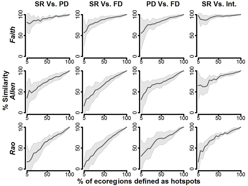
From the left to the right column we compared species richness and phylogenetic diversity hotspots (« SR Vs. PD »), species richness and functional diversity hotspots (« SR Vs. FD »), phylogenetic and functional diversity hotspots (« PD Vs. FD »), species richness and integrative hotspots (agreement between the three facets, « SR. Vs. Int. »). From the top to the bottom row we used Faith_cor, Allen_cor and Rao_cor as PD and FD. The dark continuous line represents mean percentage of congruence of hotspot lists averaged across biomes; the shaded polygon is the associated standard error of the mean. The relative congruence among hotspot lists of two biodiversity facets was determined as the number of ecoregions identified as hotspots by both, divided by the total number of ecoregions in a group.

On average, using SAR instead of PDAR/FDAR to define PD/FD hotspots marginally modified the hotspot list (Appendix S10). However, it turns out that there is still high variability between biomes. For some of these, using SAR instead of PDAR/FDAR dramatically changes the hotspot lists. Note also that the nonlinear fit of the power model alone gave relatively similar results to those obtained when using model averaging to define hotspots (Appendix S11).

Discussion

We found considerable geographical mismatches among global mammal hotspots of SR, PD and FD and, quite importantly, found that the magnitude of the mismatches depends on the index considered, which highlight the importance of considering a variety of indices (Huang et al. 2012). Mismatches were higher with Rao-based indices (Rao_cor), lower when using the Faith_cor indices and in-between for the Allen_cor indices, whatever the facet considered. This is not entirely surprising given the correlation between SR and PD/FD (high with Faith_cor, medium with Allen_cor and weak with Rao_cor).

Rodrigues et al. (2011) already pointed out a high congruence between Faith_cor PD hotspots and species richness hotspots. As a result, they concluded that incorporating phylogenetic information is not a major concern in conservation. Nevertheless, incorporating relative species coverage into the definition of multifaceted hotspots alters this conclusion. Faith_cor indices do not incorporate species abundance or coverage and give equal weight to rare and dominant evolutionary history in a given location (Chao et al., 2010). However, it seems appropriate to give less weight to particular evolutionary histories (i.e. particular branch paths) that are rare in a given ecoregion because they are less representative than a widespread species in this ecoregion. Allen_cor and Rao_cor indices give more weight to a given branch if it is long and well represented in an ecoregion. For instance, hotspots defined using the PD Rao_cor are mostly concentrated in the Australasian realm because of the presence of marsupials. This group has a unique evolutionary history since they diverged 147 millions years ago from placentals (extant eutherians, grouping the majority of mammals) and are widely distributed (i.e. large coverage) through the Australasian ecoregions (and not in South American ecoregions). These results are congruent with those of a recent study revealing important mismatches between global mammal trait variance hotspots and SR (Huang et al., 2012). Although these authors used a different approach (they used grid cells as geographical units and did not use information about species coverage) these close results are probably explained by the fact that Rao_cor indices are linked to a measure of variance (Pavoine & Bonsall, 2011). We also showed that the use of body mass alone to define FD hotspots is not sufficient to match the FD hotspots defined with our complete set of traits but that it still represent an acceptable approximation. We also showed that PD and FD hotspots are not always congruent, suggesting that PD is not necessarily a good surrogate for FD (at least for the functional traits selected here).

As well as defining hotspots, DARs have been shown to be useful in both applied and fundamental ecology. We found that Faith_cor PDAR and FDAR generally reach their maximum faster than SAR (Cumming & Child, 2009). This result was expected since Faith_cor PD and FD explicitly account for redundancy between species while SR does not. More specifically, it is possible that small sample areas already contain a broad set of phylogenetic history and functional diversity (e.g. a mouse and an elephant), whereas large sample areas contain relatively more redundant species (e.g. several species of mice) and thus PDAR/FDAR reach their maximum faster than SAR.

Morlon et al. (2011) obtained a similar result for PDAR on nested Mediterranean plant communities ranging from 6.25m² to 400m² of spatial extent. They used power law (see Appendix S1) to model PDAR and SAR and found that the rate of increase in Faith PD with area (z_PDAR) was slower that in SR (z_SAR). When standardizing DARs, PDAR is above SAR if zPDAR < z_SAR. They showed that protected areas in Australian Mediterranean-like regions (representing 13% of the regions) capture 72% of PD, but only 56% of species richness, indicating that PDAR accumulates total diversity faster than SAR.

Our results show that if only a fraction of the total biome area is protected, the percentage of remaining PD (compared to the initial PD) will be higher than the percentage of remaining species. If we consider that PD or FD are better predictors of ecosystem functioning, resistance or resilience (Cadotte et al., 2009; Gravel et al., 2012) than SR, it means that ecosystem features might be more robust to species loss than previously predicted (but see Mouillot et al. (2013)).

We also found that a key feature of a comprehensive measure of diversity is that when rarely represented evolutionary history is progressively removed (i.e. using different values of q), the differences between PDAR/FDAR and SAR increase. In other words, PD/FD of abundant lineages reaches its maximum faster than when considering all lineages having the same coverage. This result suggests that the evolutionary history or functional traits of well-represented taxa are relatively more rapidly sampled when area increases. For example, branches of major mammal lineages (e.g. bats, rodents or carnivores) are probably already well sampled in small ecoregions and thus PD or FD reaches their maximum faster than TD in larger sample areas. It follows that well represented functional/phylogenetic biodiversity might be robust to habitat loss, a point that is not detected when considering all lineages having the same coverage.

Although SARs have been thoroughly investigated (Scheiner, 2003), we showed that there is not a single best model that fits all the data. Thus the automatic use of a single model (traditionally the linear version of power model) is not justified. Conversely, to date PDAR and FDAR have been subject to very little investigation (but see Cumming & Child, 2009; Morlon et al., 2011; Helmus & Ives, 2012; Wang et al., 2011). Here, given the important variability across biomes and indices, we also show that a single best model does not exist for PDAR and FDAR. Nevertheless the model-averaging framework allows taking into account these uncertainties and we used an averaged prediction to remove the area effect on PD/FD. We also asked whether the averaged SAR could be a good proxy of the averaged PDAR/FADR to remove this area effect to define PD/FD hotspots. We demonstrated that there is a notable difference between PD/FD hotspot lists defined using PDAR/FDAR and those defined using SAR, suggesting that the construction of PDAR/FDAR is required to define functionally- or phylogenetically-based hotspots and that SAR alone can not be used for this purpose.

We constructed DARs using a particular experimental design (Scheiner, 2003) but we are aware that all methodologies for constructing DARs have their own drawbacks and we suggest that the next challenge in the study of large scale multifaceted DARs is to test different methodological designs. For example the strictly nested design (SNQ) of Storch et al. (2012) seems particularly interesting to analyse. Nevertheless, since our work was about delineating hotspots of diversity, we had to construct DARs using a non-overlapping design.

Conclusion

Here we used a unified framework for building large scale DARs for each facet of mammal diversity. The spatial scaling of each facet revealed that PD/FD reach their maximal diversity faster than SAR suggesting that PD/FD might be less vulnerable than SR to habitat loss. In addition, we extracted the area effect on the diversity of individual terrestrial ecoregions to identify multifaceted hotspots of diversity. We showed that multifaceted hotspots are not necessarily congruent and, thus, that SR, PD and FD are not necessarily good surrogates for each other, especially when considering species relative coverage. Although global hotspot identification is important as an initial coarse-scale assessment of the conservation value of different regions (Lamoreux et al., 2006), several challenges would need to be addressed before our results could be directly transferred into conservation planning actions.

Biosketch

F. Mazel is a PhD student mostly interested in macroecology and macroevolution. Specifically, he aims at describing and understanding the distribution of biodiversity in the light of ecology, evolution, paleontology and paleoclimatology.

References

- Allen B, Kon M, Bar-Yam Y. A new phylogenetic diversity measure generalizing the shannon index and its application to phyllostomid bats. The American Naturalist. 2009;174:236–243. doi: 10.1086/600101. [DOI] [PubMed] [Google Scholar]
- Bininda-Emonds ORP, Cardillo M, Jones KE, MacPhee RDE, Beck RMD, Grenyer R, Price SA, Vos RA, Gittleman JL, Purvis A. The delayed rise of present-day mammals. Nature. 2007;446:507–12. doi: 10.1038/nature05634. [DOI] [PubMed] [Google Scholar]
- Burnham KP, Anderson DR. Model selection and inference: a practical information-theoretic approach. Springer-Verlag; 1998. [Google Scholar]
- Cadotte M, Cavender-Bares J, Tilman D, Oakley T. Using phylogenetic, functional and trait diversity to understand patterns of plant community productivity. PLoS One. 2009;4:e5695. doi: 10.1371/journal.pone.0005695. [DOI] [PMC free article] [PubMed] [Google Scholar]
- Ceballos G, Ehrlich PR. Global mammal distributions, biodiversity hotspots, and conservation. Proceedings of the National Academy of Sciences of the United States of America. 2006;103:19374–19379. doi: 10.1073/pnas.0609334103. [DOI] [PMC free article] [PubMed] [Google Scholar]
- Chao A, Chiu CH, Jost L. Phylogenetic diversity measures based on Hill numbers. Philosophical Transactions of the Royal Society of London. Series B, Biological Sciences. 2010;365:3599–3609. doi: 10.1098/rstb.2010.0272. [DOI] [PMC free article] [PubMed] [Google Scholar]
- Chown S, Gaston K. Areas, cradles and museums: the latitudinal gradient in species richness. Trends in Ecology & Evolution. 2000;15:311–315. doi: 10.1016/s0169-5347(00)01910-8. [DOI] [PubMed] [Google Scholar]
- Cumming GS, Child MF. Contrasting spatial patterns of taxonomic and functional richness offer insights into potential loss of ecosystem services. Philosophical Transactions of the Royal Society of London. Series B, Biological Sciences. 2009;364:1683–1692. doi: 10.1098/rstb.2008.0317. [DOI] [PMC free article] [PubMed] [Google Scholar]
- Davies TJ, Buckley LB. Phylogenetic diversity as a window into the evolutionary and biogeographic histories of present-day richness gradients for mammals. Philosophical Transactions of the Royal Society of London. Series B, Biological Sciences. 2011;366:2414–2425. doi: 10.1098/rstb.2011.0058. [DOI] [PMC free article] [PubMed] [Google Scholar]
- Faith DP. Conservation evaluation and phylogenetic diversity. Biological Conservation. 1992;61:1–10. [Google Scholar]
- Forest F, Grenyer R, Rouget M, Davies TJ, Cowling RM, Faith DP, Balmford A, Manning JC, Procheş S, van der Bank M, Reeves G, Hedderson TAJ, Savolainen V. Preserving the evolutionary potential of floras in biodiversity hotspots. Nature. 2007;445:757–760. doi: 10.1038/nature05587. [DOI] [PubMed] [Google Scholar]
- Fritz SA, Bininda-Emonds ORP, Purvis A. Geographical variation in predictors of mammalian extinction risk: big is bad, but only in the tropics. Ecology letters. 2009;12:538–49. doi: 10.1111/j.1461-0248.2009.01307.x. [DOI] [PubMed] [Google Scholar]
- Gaston KJ. The Structure and Dynamics of Geographic Ranges. Oxford University Press; Oxford, UK: 2003. [Google Scholar]
- Gaston KJ, Blackburn TM, Greenwood JJD, Gregory RD, Quinn RM, Lawton JH. Abundance-occupancy relationships. Journal of Applied Ecology. 2000;37:39–59. [Google Scholar]
- Gravel D, Bell T, Barbera C, Combe M, Pommier T, Mouquet N. Phylogenetic constraints on ecosystem functioning. Nature communications. 2012;3:1117. doi: 10.1038/ncomms2123. [DOI] [PubMed] [Google Scholar]
- Groves C. Drafting a conservation blueprint: a practitioner’s guide to planning for biodiversity. Island Press; Washington, D.C.: 2003. [Google Scholar]
- Guilhaumon F, Gimenez O, Gaston KJ, Mouillot D. Taxonomic and regional uncertainty in species-area relationships and the identification of richness hotspots. Proceedings of the National Academy of Sciences of the United States of America. 2008;105:15458–15463. doi: 10.1073/pnas.0803610105. [DOI] [PMC free article] [PubMed] [Google Scholar]
- Hawkins BA, Diniz-Filho JAF, Jaramillo CA, Soeller SA. Post-Eocene climate change, niche conservatism, and the latitudinal diversity gradient of New World birds. Journal of Biogeography. 2006;33:770–780. [Google Scholar]
- Hawkins BA, McCain CM, Davies TJ, Buckley LB, Anacker BL, Cornell HV, Damschen EI, Grytnes J-AA, Harrison S, Holt RD, Kraft NJB, Stephens PR, et al. Different evolutionary histories underlie congruent species richness gradients of birds and mammals. Journal of Biogeography. 2012;39:825–841. [Google Scholar]
- Helmus MR, Ives AR. Phylogenetic diversity–area curves. Ecology. 2012;91:31–43. [Google Scholar]
- Huang S, Stephens PR, Gittleman JL. Traits, trees and taxa: global dimensions of biodiversity in mammals. Proceedings of the Royal Society, Series B. 2012;279:4997–5003. doi: 10.1098/rspb.2012.1981. [DOI] [PMC free article] [PubMed] [Google Scholar]
- Isaac NJB, Turvey ST, Collen B, Waterman C, Baillie JEM. Mammals on the EDGE: conservation priorities based on threat and phylogeny. PLoS One. 2007;2:e296. doi: 10.1371/journal.pone.0000296. [DOI] [PMC free article] [PubMed] [Google Scholar]
- Jost L. Entropy and diversity. Oikos. 2006;113:363–375. [Google Scholar]
- Lamoreux JF, Morrison JC, Ricketts TH, Olson DM, Dinerstein E, McKnight MW, Shugart HH. Global tests of biodiversity concordance and the importance of endemism. Nature. 2006;440:212–214. doi: 10.1038/nature04291. [DOI] [PubMed] [Google Scholar]
- Loreau M, Naeem S, Inchausti P. Biodiversity and ecosystem functioning: synthesis and perspectives. Oxford University Press; USA: 2002. [Google Scholar]
- Mittermeier RA, Gil PR, Hoffman M, Pilgrim J, Brooks T, Mittermeier CG, Lamoreux J, Da Fonseca GAB. In: Hotspots Revisited. Cemex, editor. Mexico city: 2004. [Google Scholar]
- Mittermeier RA, Mittermeier CG, Brooks TM, Pilgrim JD, Konstant WR, da Fonseca G. a B., Kormos C. Wilderness and biodiversity conservation. Proceedings of the National Academy of Sciences of the United States of America. 2003;100:10309–10313. doi: 10.1073/pnas.1732458100. [DOI] [PMC free article] [PubMed] [Google Scholar]
- Morlon H, Schwilk DW, Bryant JA, Marquet PA, Rebelo AG, Tauss C, Bohannan BJM, Green JL. Spatial patterns of phylogenetic diversity. Ecology letters. 2011;14:141–149. doi: 10.1111/j.1461-0248.2010.01563.x. [DOI] [PMC free article] [PubMed] [Google Scholar]
- Mouillot D, Bellwood DR, Baraloto C, Chave J, Galzin R, Harmelin-vivien M, Kulbicki M, Lavergne S, Lavorel S, Mouquet N, Paine TCE, Renaud J, Thuiller W. Rare species support vulnerable functions in high-diversity ecosystems. PLOS Biology. 2013;11:e1001569. doi: 10.1371/journal.pbio.1001569. [DOI] [PMC free article] [PubMed] [Google Scholar]
- Mouquet N, Devictor V, Meynard CN, Munoz F, Bersier L-FF, Chave J, Couteron P, Dalecky A, Fontaine C, Gravel D, Hardy OJ, Jabot F, Lavergne S, Leibold M, Mouillot D, Münkemüller T, Pavoine S, Prinzing A, Rodrigues ASL, Rohr RP, Thébault E, Thuiller W, et al. Ecophylogenetics: advances and perspectives. Biological Reviews. 2012;87:769–785. doi: 10.1111/j.1469-185X.2012.00224.x. [DOI] [PubMed] [Google Scholar]
- Myers N, Mittermeier RA, Mittermeier CG, da Fonseca GA, Kent J. Biodiversity hotspots for conservation priorities. Nature. 2000;403:853–858. doi: 10.1038/35002501. [DOI] [PubMed] [Google Scholar]
- Olson DM, Dinerstein E. The Global 200: a representation approach to conserving the Earth’s most biologically valuable ecoregions. Conservation Biology. 1998;12:502–515. [Google Scholar]
- Olson DM, Dinerstein E, Wikramanayake ED, Burgess ND, George VNP, Underwood ED, D’amico J, Itoua I, Strand HE, Morrison JC, Powell GVN, Underwood EC, D’amico J. a., Loucks CJ, Allnutt TF, Ricketts TH, Kura Y, Lamoreux JF, Wettengel WW, Hedao P, Kassem KR. Terrestrial Ecoregions of the World: A New Map of Life on Earth. BioScience. 2001;51:933–938. [Google Scholar]
- Orme CDL, Davies RG, Burgess M, Eigenbrod F, Pickup N, Olson VA, Webster AJ, Ding T-S, Rasmussen PC, Ridgely RS, Stattersfield AJ, Bennett PM, Blackburn TM, Gaston KJ, Owens IPF. Global hotspots of species richness are not congruent with endemism or threat. Nature. 2005;436:1016–1019. doi: 10.1038/nature03850. [DOI] [PubMed] [Google Scholar]
- Pavoine S, Bonsall MB. Measuring biodiversity to explain community assembly: a unified approach. Biological Reviews. 2011;86:792–812. doi: 10.1111/j.1469-185X.2010.00171.x. [DOI] [PubMed] [Google Scholar]
- Petchey OL, Gaston KJ. Functional diversity: back to basics and looking forward. Ecology letters. 2006;9:741–758. doi: 10.1111/j.1461-0248.2006.00924.x. [DOI] [PubMed] [Google Scholar]
- R Development Core Team . R: A Language and Environment for Statistical Computing. Vienna, Austria: 2010. [Google Scholar]
- Rao RC. Diversity and dissimilarity coefficients: a unified approach. Theoretical population biology. 1982;21:24–43. [Google Scholar]
- Reid WV. Biodiversity hotspots. Trends in Ecology and Evolution. 1998;13:275–280. doi: 10.1016/s0169-5347(98)01363-9. [DOI] [PubMed] [Google Scholar]
- Rodrigues ASL, Grenyer R, Baillie JEM, Bininda-Emonds ORP, Gittlemann JL, Hoffmann M, Safi K, Schipper J, Stuart SN, Brooks T. Complete, accurate, mammalian phylogenies aid conservation planning, but not much. Philosophical Transactions of the Royal Society of London. Series B, Biological Sciences. 2011;366:2652–2660. doi: 10.1098/rstb.2011.0104. [DOI] [PMC free article] [PubMed] [Google Scholar]
- Safi K, Cianciaruso MV, Loyola RD, Brito D, Armour-Marshall K, Diniz-Filho JAF. Understanding global patterns of mammalian functional and phylogenetic diversity. Philosophical Transactions of the Royal Society of London. Series B, Biological Sciences. 2011;366:2536–2544. doi: 10.1098/rstb.2011.0024. [DOI] [PMC free article] [PubMed] [Google Scholar]
- Scheiner SM. Six types of species-area curves. Global Ecology and Biogeography. 2003;12:441–447. [Google Scholar]
- Sekercioglu CH. Ecosystem functions and services. In: Sodhi PR, Ehrlich N. S. and, editors. Conservation Biology for All. Oxford University Press; Oxford United Kingdom: 2010. pp. 45–72. [Google Scholar]
- Srivastava DS, Cadotte MW, MacDonald AAM, Marushia RG, Mirotchnick N. Phylogenetic diversity and the functioning of ecosystems. Ecology letters. 2012;15:637–48. doi: 10.1111/j.1461-0248.2012.01795.x. [DOI] [PubMed] [Google Scholar]
- Storch D, Keil P, Jetz W. Universal species-area and endemics-area relationships at continental scales. Nature. 2012;488:78–81. doi: 10.1038/nature11226. [DOI] [PubMed] [Google Scholar]
- Tjørve E. Shapes and functions of species-area curves (II): a review of new models and parameterizations. Journal of Biogeography. 2009;36:1435–1445. [Google Scholar]
- Triantis KA, Guilhaumon F, Whittaker RJ. The island species-area relationship: biology and statistics. Journal of Biogeography. 2012;39:215–231. [Google Scholar]
- Wang X, Wiegand T, Wolf A, Howe R, Davies SJ, Hao Z. Spatial patterns of tree species richness in two temperate forests. Journal of Ecology. 2011;99:1382–1393. [Google Scholar]
- Webb CO, Ackerly DD, McPeek MA, Donoghue MJ. Phylogenies and Community Ecology. Annual Review of Ecology, Evolution, and Systematics. 2002;33:475–505. [Google Scholar]
- Wiens JJ, Pyron RA, Moen DS. Phylogenetic origins of local-scale diversity patterns and the causes of Amazonian megadiversity. Ecology letters. 2011;14:643–652. doi: 10.1111/j.1461-0248.2011.01625.x. [DOI] [PubMed] [Google Scholar]
Associated Data
This section collects any data citations, data availability statements, or supplementary materials included in this article.