

SUMMARY
The idea of bridging in dose-finding studies is closely linked to the problem of group heterogeneity. There are some distinctive features in the case of bridging which need to be considered if efficient estimation of the maximum tolerated dose (MTD) is to be accomplished. The case of two distinct populations is considered. In the bridging setting we usually have in mind two studies, corresponding to the two populations. In some cases, the first of these studies may have been completed while the second has yet to be initiated. In other cases, the studies take place simultaneously and information can then be shared among the two groups. The methodological problem is how to make most use of the information gained in the first study to help improve efficiency in the second. We describe the models that we can use for the purpose of bridging and study situations in which their use leads to overall improvements in performance as well as cases where there is no gain when compared to carrying out parallel studies. Simulations and an example in pediatric oncology help to provide further insight.
Keywords: Bridging, Calibration, Clinical trials, Continual Reassessment Method, Dose escalation, Dose finding studies, Pediatric trials, Pharmacokinetics, Phase 1 trials, Toxicity
1 Introduction
It is not unusual to want to carry out a dose-finding study in some well defined population when, already, a similar study has been completed in some other population. Here, the word similar is not sharply defined but we typically have in mind the same drug or combination of drugs, and often the same range of possible dose levels and, mostly, the same clinical setting. The population we have in mind may have been deliberately omitted from the original study, i.e., failed to meet inclusion criteria, or may not have seemed relevant to the earlier, completed, study. Until relatively recently, it was not even considered necessary to carry out a dose-finding study in children and the maximum tolerated dose (MTD), established for an adult population was simply extrapolated to children on the basis of some elementary adjustment such as ratio of the average body surface area for adults compared to that for children. It was not felt necessary to actual carry out a real dose finding study on the children themselves. However, the growing realisation that an MTD, estimated in this way, was yet more unreliable than that estimated on the basis of an actual study, has prompted the regulatory authorities to increasingly require that a study be carried out on the children themselves.
A number of different situations can come under this heading. It may be that we wish to carry out simultaneously two studies but that we anticipate potentially large imbalances in recruitment. As far as the second study is concerned, we might simply just ignore the first study, and view the second one as an independent study in its own right. The difficulty here, at least in the case of pediatrics, is that the number of patients available for study can be as much as an order of magnitude less than those available for the original study. More generally, even when sample size is not the major consideration, it can make sense to take whatever information we can from the first study for use in the second study. The question which then arises is how to make the best use this information. Statistically we would like to use the information in such a way that good, efficient use is made of this information provided from the first study, while, at the same time, the recommended MTD of the second study is essentially located by virtue of information obtained mostly during the second study. This can require some care on the part of the statistician and the use of models that specifically involve a bridging parameter.
We can think of the above set-up as one of bridging in the context of dose finding. The feature that most distinguishes a bridging dose finding study from a regular dose finding study can be summarized via their different levels of precision. A regular dose finding study, at the outset, might allow the possibility that any one of 6, 8 or as many as 12 levels could equally well correspond to the MTD. For a bridging dose finding study, the MTD is most likely to be the same as that established in the first study, one level removed from that level or, less frequently, two levels removed from that level. More than two levels removed would be unusual to the point that it may cast doubt on the reliability of the estimated MTD for the original population. Whether carried out simultaneously, or whether staggered in time, the difficulty is to correctly make use of information that is being, or has been, accrued in the first population to help improve estimation and dose allocation in the second. The trick is to obtain the correct balance between the information being gathered in the two studies so that the second study is neither dominated by the first, nor is it left to its own devices when resources (patients) are rare.
Geoerger (2005) made use of the two-sample CRM in which there were two levels of groupings; the first between the children and the adults and the second within the children themselves. This enabled a single rather than two separate trials with dose-escalations in two stratified groups. The more efficient use of the data allowed both groups to be evaluated simultaneously, sharing information and thereby improving overall identification of both MTDs. The MTDs were estimated more accurately since they are identified on the basis of all collected observations and not just distinct subsets. The CRM determined level 2 for the nonheavily pretreated children and level 1 for the heavily pretreated children as recommended doses for the combination. The classical dose escalation would have determined level 1 and minus 1, respectively, which are below the single MTD doses of temozolomide for these cohorts. In this case at least, it appears as though the classical design would have been too conservative in its estimate of MTDs. We return to the examples in Section 4. Before that, we describe in the next two sections the models that can be made use of here and the implications they have for efficiency depending on the true situations that we may be facing.
2 METHODS
2.1 Simple and extended dose-finding models
Let there be k ordered doses; d1, … dk. The dose levels which can be multi dimensional are supposed ordered in terms of the probabilities, R(di), for toxicity at each of the levels, i.e. R(di) ≤ R(dj) whenever i < j. The maximum tolerated dose (MTD), and the sequential ‘target’ dose for a model-based design is denoted d0 where d0 ∈ {d1, … dk} is that dose having an associated probability of toxicity, R(d0), as close as we can get to some target “acceptable” toxicity rate θ. Specifically we define d0 ∈ {d1, … dk} such that
| (1) |
A number of other definitions, corresponding to a loosening of the above requirement, could be considered. Designs that put emphasis on controlling overdosing (EWOC designs) consider a slightly different distance measure. These designs target a lower percentile, say 25%, rather than the median or mean of the posterior distribution (Chu, Lin and Shih 2009). The purpose of such an asymmetric allocation rule is to obtain a lower target rate and the methodology we present here can be used in the context of EWOC designs with no essential modification. The very same models put forward here could be used equally well in an EWOC context and the only difference would be in the dose allocation since the distance may be different. To what extent final recommendations and accuracy is impacted is a question as yet, to the authors’ knowledge, unexplored.
The binary indicator Yj takes the value 1 in the case of a toxic response for the j th entered subject (j = 1, … n) and 0 otherwise. The dose for the j th entered subject, Xj is viewed as random taking values xj ∈ {d1, … dk}; j = 1, …, n. Thus Pr (Yj = 1|Xj = xj) = R(xj). The study’s aim is to estimate d0 while sequentially treating each individual at the current best estimate of the MTD. The continual reassessment method (CRM) models R(xj), the true probability of toxic response at Xj = xj; xj ∈ {d1, … dk} by
| (2) |
for some one parameter model ψ(xj, a) and a defined on the set
 (O’Quigley, Pepe and Fisher 1990). For every a, ψ(x, a) should be monotone increasing in x and, for any x, ψ (x, a) should be monotone in a. For every di there exists some ai ∈
such that R(di) = ψ (di, ai), i.e. the one parameter model is rich enough, at each dose, to exactly reproduce the true probability of toxicity at that dose. We have a lot of flexibility in our choice for ψ (x, a). The simple choice:
, where i runs from 1 to k, and where 0 < α1 < … < αk < 1 and −∞ < a < ∞, has worked well over a range of applied studies. The level chosen for the n + 1 th patient, who is hypothetical, is also our estimate of d0. After having included j subjects, and given the set Ωj of outcomes so far, we can calculate a posterior distribution for a which we denote by f(a | Ωj). We then induce a posterior distribution for ψ(di, a), i = 1, …, k, from which we can obtain summary estimates of the toxicity probabilities at each level so that;
(O’Quigley, Pepe and Fisher 1990). For every a, ψ(x, a) should be monotone increasing in x and, for any x, ψ (x, a) should be monotone in a. For every di there exists some ai ∈
such that R(di) = ψ (di, ai), i.e. the one parameter model is rich enough, at each dose, to exactly reproduce the true probability of toxicity at that dose. We have a lot of flexibility in our choice for ψ (x, a). The simple choice:
, where i runs from 1 to k, and where 0 < α1 < … < αk < 1 and −∞ < a < ∞, has worked well over a range of applied studies. The level chosen for the n + 1 th patient, who is hypothetical, is also our estimate of d0. After having included j subjects, and given the set Ωj of outcomes so far, we can calculate a posterior distribution for a which we denote by f(a | Ωj). We then induce a posterior distribution for ψ(di, a), i = 1, …, k, from which we can obtain summary estimates of the toxicity probabilities at each level so that;
| (3) |
Replacing R(d0) by R̂(di) in Equation 1, we can now decide which dose level to allocate to the (j + 1)th patient. In this context the starting level di should be such that
 ψ(di,u)g(u)du=θ. This may be a difficult integral equation to solve and, practically, we might take the starting dose to be obtained from ψ (di, μ0) = θ where μ0=
ug(u)du.
ψ(di,u)g(u)du=θ. This may be a difficult integral equation to solve and, practically, we might take the starting dose to be obtained from ψ (di, μ0) = θ where μ0=
ug(u)du.
Suppose now that, instead of the single model of Equation 2, we have some class of models of interest and we denote these models as ψm(xj, a) for m = 1, …, M where there are a total of M possible models. In particular, we might consider where i = 1, …, k; m = 1, …, M and where 0 < αm1 < … < αmk < 1 and −∞ < a < ∞, as an immediate generalization of the single model described at the beginning of the section. Further, we may wish to take account of any prior information concerning the plausibility of each model and so introduce π(m), m = 1, …, M, where π(m) ≥ 0 and where Σmπ(m) = 1. In the simplest case where each model is weighted equally, we would take π(m) = 1/m. If the data are to be analyzed under model m then, following the inclusion of j patients, the logarithm of the likelihood, can be written as:
| (4) |
where any terms not involving the parameter a have been equated to zero. Under model m we obtain a summary value of the parameter a, in particular the maximum of the posterior mode and we refer to this as âmj. Given the value of âmj under model m we have an estimate of the probability of toxicity at each dose level di via: R̂(di) = ψm (di, âmj), (i = 1, …, k). On the basis of this formula, and having taken some value for m, the dose to be given to the (j + 1) th patient, xj+1 is determined. Thus, we need some value for m and we make use of the posterior probabilities of the models given the data Ωj. Denoting these posterior probabilities by π (m|Ωj) then:
| (5) |
In some cases the π(m|Ωj) are only of very indirect interest, such as using several models and then averaging to decide on the best current, running, estimate of the MTD. In other cases the π(m|Ωj) can play a more central role and we will want to say something about m itself as we make progress. Once m, our indicator over potential models, takes values greater than one, then we consider that we are dealing with “extended” models. Yuan and Yin (2011) adopted this view as a way to increase robustness to model choice in the single group situation. Models that may appear to be providing an awkward fit would be weighted down in favour of ones that, at least locally, provide a better description of the accumulating observations. Our purpose is different here but the idea of focusing attention on a limited small collection of models is similar. A reviewer of an earlier version of this work pointed out the fact that the particular models that we explore here, based on a very limited number of possibilities for the parameter describing heterogeneity, connects strongly to work on discretized priors. This is a valuable insight because not only can we go from a situation of a continuous parameter to one taking only a few discrete values, but we can also proceed in the opposite direction, that is from a parameter with discrete values to one where, at least locally, we can construct a continuous parameterization. We go further and make the dose-toxicity function to be twice differentiable in such local neighbourhoods. The purpose is a theoretical and not an operational one. In practice, it can be very difficult to locate the maximum when there is little information and a continuous parameter space. A few discrete possible values for the parameter transforms this potentially awkward and unstable situation into a very simple and tractable one. So, this is what we do in practice. As far as theory goes however, it is more useful to work with a twice differentiable function of the heterogeneity parameter. We make use then of two different models noting that, at a given dose level the models are effectively equivalent.
2.2 Models accounting for group heterogeneity
As in other types of clinical trials we are essentially looking for an average effect. Patients naturally differ in the way they may react to a treatment and, although hampered by small samples, we may sometimes be in a position to specifically address the issue of patient heterogeneity. In many actual dose finding studies it is more likely to be the rule than the exception that there exists significant heterogeneity among the patients. The goal of fully accounting for all sources of heterogeneity would coincide with that of individualized dose finding, a laudable although, at this stage, an unrealistic goal. A lesser goal is that of combining patients into rough prognostic groups and some of these immediately suggest themselves. Common examples are dividing the patients into heavily pre-treated and less heavily pre-treated patient groups, or, possibly, dividing the groups on the basis of adult and adolescent groups. One example occurs in patients with acute leukaemia where it has been observed that children will better tolerate more aggressive doses (standardized by their weight) than adults. Likewise, heavily pre-treated patients are more likely to suffer from toxic side effects than lightly pre-treated patients. In such situations we may wish to carry out separate trials for the different groups in order to identify the appropriate MTD for each group. Otherwise we run the risk of recommending an “average” compromise dose level, too toxic for a part of the population and suboptimal for the other. Usually, clinicians carry out two separate trials or split a trial into two arms after encountering the first DLTs when it is believed that there are two distinct prognostic groups. This has the disadvantage of failing to utilize information common to both groups. The most common situation is that of two samples where we aim to carry out a single trial keeping in mind potential differences between the two groups. A multi-sample CRM is a direct generalization although we must remain realistic in terms of what is achievable in the light of the available sample sizes.
O’Quigley, Shen and Gamst (1999) focus mostly on models for the two group case, since this case is the most common and there are not usually enough resources, in terms of patient numbers, to deal with more complex structures. Elaborating higher dimensional models, at least conceptually, is straightforward. The dose toxicity model is written;
| (6) |
for i = 1, …, k) and where the parameter b measures to some extent the difference between the groups. where, again, 0 < α1 < … < αk < 1; −∞ < a < ∞, −∞ < b < ∞ and Z is a binary group indicator. Asymptotic theory is cumbersome for these models but consistency can be shown under restrictive assumptions (O’Quigley, Shen and Gamst 1999). An alternative approach, in harmony with the underlying CRM idea of exploiting underparametrized models, is to be even more restrictive than allowed by the above regression models. Rather than allow for a large, possibly infinite, range of potential values for the second parameter b, measuring differences between the groups, the differences themselves are taken from a very small finite set. Since, in any event, if the first group finishes with a recommendation for some level, d0 say, then the other group will be recommended either the same level or some level, one, two or more, steps away from it. The idea is to parameterize these steps directly. The indices themselves are modeled and the model is less cluttered if we work with log ψ(di, a) rather than ψ(di, a) writing;
| (7) |
where
the last three terms in the above expression taking care of edge effects. The problem of edge effects only arises with the discretely parameterized version of the heterogeneity model. If, for example, the MTD for the first group is estimated at the highest level then the question arises to the meaning of any Δ other than zero. So, the allowable values of Δ may depend themselves on the dose. There is more than one way of dealing with this feature. Here, we add skeleton values to the highest level for group 2 and we add the same number of levels before level 1. Another possibility would be to simply pile up levels on the highest for group 2 and the lowest for group 1 according to the value of Δ. Such a discrete model would no longer be equivalent to a continuous analogue described here and, for this reason, we have not studied that approach more deeply.
As already pointed out, it is readily seen that the discrete and continuous model descriptions are in fact identical as far as model structure is concerned and only differ through the support of the distribution allowed for the parameter. Posterior or likelihood forms will be identical at each of the dose levels. In a Bayesian setting that appears quite natural. In a classical setting it appears less natural but can be shown formally by re-writing the model expression so that for m = 1, we can write and, for m = 2, we write when allowing b to be continuous. When the shift parameter Δ is discrete, then for m = 1, and for m = 2, we write . It is easy to put a discrete prior on Δ, possibly giving a preponderance of weight to Δ = 0 and only allowing one or two dose level shifts if the evidence of the accumulating data points strongly in that direction. To indicate that the MTD may depend on the group we write it as dZ0 for Z = 0, 1.
Inference for a bridging model
Bridging can arise in different forms; simultaneous parallel studies, studies in which the second group begins after the first group has completed inclusions and studies that might overlap to some degree. There are two important concepts that are specific to bridging. These can be expressed as two fundamental parameters, one of which is to be estimated whereas the other is a fixed design parameter.
Bridging parameters
The first parameter can be described as the bridging parameter itself and this connects the two groups both statistically and operationally. This parameter can take different forms and we have in mind mostly the form given above where the bridging parameter can be expressed as the model indicator m. This provides the link between the two groups with the special case m = 1 corresponding to an absence of a link, i.e., two independent groups. A number of examples are given in the above section and it is easy to create other model constructions corresponding to any particular set-up. A very general expression involving m would lose transparency and it seems best to deal with each situation on a case by case basis. The second parameter is a design parameter called the diminishing parameter. It quantifies how much the information provided by the first group is diluted. Unlike the bridging parameter m, the diminishing parameter is not to be estimated and is fixed as part of the design. The diminishing parameter is denoted w(n1) where w(n1) is a multiplicative factor of the log likelihood of the first group and (1 −w(n1)) is a multiplicative factor for the second group. A value one means that all the information of the first group is used. A value 1/2 means essentially that, as far as the second group is concerned, it is as though the first group had been constructed using a sample size n1/2 rather than n1. The idea is immediately extended to a more sophisticated type of diminishing that can impact the levels differently. We would then have a different diminishing parameter, wi(n), for each level i = 1, …, k. The weight wi(n), will multiply each estimating equation at each dose level i. For more details refer to O’Quigley 2005, Equation 4. However, such generalization is unlikely to be used much in practice.
Efficiency gains versus potential bias
As for any statistical model we would expect to make efficiency gains when the model correctly takes into account non-negligible differences between the groups. The grouping variable can be viewed as an indicator of a source of potentially significant variability so that, correctly accounting for the grouping can lead to important increases in precision. Under a multinormal linear model, it is possible that there be no bias but the precision of estimation for other factors can nonetheless be reduced. We need also consider what happens when, we try to account for a source of variability which turns out not to be related to the outcome of interest. In these cases, the extra estimation effort, that is not in fact needed, will usually lead to a reduction in efficacy. These questions become yet more difficult in a context where the working models are incorrectly specified. The issue of what happens to the overall dose-toxicity function is a difficult one to deal with, and, in any event, is not really very relevant. It is more important to know what happens at the estimated MTD. This can be studied but we are not able to make the usual appeal to established results from nested models in the context of likelihood theory. Such techniques fail when models are misspecified and we need to make use of different techniques to those classically used.
Recalling the general expression for the bridging model we have,
where, as usual, Y is the indicator of toxic response, x indicates the dose at which experimentation is being carried out, and Z = 0, 1 is a binary variable identifying the groups. The model corresponds to the situation in which information is being borrowed or shared between the groups. If no information is to be shared then no bridging model is required and we could express the situation as one where there are two independent groups so that,
where b parametrizes the second group when considered to be independent from the first. The most common situation, potentially leading to bias, is one where there exist real group differences but these are either assumed to not exist or, otherwise, to not be important enough to model. As a result the two groups are put together in a single combined model where,
The groups are not necessarily included simultaneously and the final inclusion for the first group can take place before the first inclusion for the second group. The inclusions nonetheless proceed as though there were just one group so that the first patient from the second group contributes the exact same information to the likelihood as would an extra patient, had the patient been added on to the first group. Estimation is based on maximum likelihood (under non-standard conditions) and the target parameters are denoted a0 and b0, and is the underlying probability of toxicity (Ri(·)) at the target dose ( ) for group i = 1, 2. Whichever scheme is adopted, correct dose recommendation relies in large part on precise estimation of the parameters in the model. The asymptotic variances for the corresponding estimates give some indication of their relative precision and thus, at least from a theoretical point of view, it is sufficient to base comparisons of the various schemes on comparisons of asymptotic variance.
The optimal scheme when the two groups are homogeneous, i.e., when there are no differences between the two groups is based on the single model. This makes the most use of the all of the information available. The approach is consistent under some mild regularity conditions and some model restrictions that are respected by the models used here (Shen and O’Quigley 1996). The estimate ân of the parameter a0 is asymptotically normal with a large sample variance
| (8) |
in which . On the other hand, we can perform two independent experiments – one with a fraction p of the subjects in group 1 and the other group with 1−p. The parameter estimates are asymptotically normal with variances
| (9) |
using ψ1 as the model for the two groups, and a0, b0 are the true population values. The large sample variance will be inflated by at least (1/max(p, (1−p))) but by properly averaging the two parameter estimates we can recover the “optimal” asymptotic variance in Equation 8. This means that we have not lost anything asymptotically. For finite samples, of course, there will be some loss of information. Since the bridging model takes advantage of the information common to both groups, it will do better than running separate trials and, once more, by averaging, we can recover the expression for the asymptotic variance in Equation 8 just above.
When the two groups really are different, a pooled approach will not generally be consistent since the estimated MTD will converge to a weighted average of the target doses for the two groups. As far as efficiency is concerned, the appropriate comparison is then between the bridging model and carrying out two trials separately. Given a total of n patients already treated, we will assume that the first n1 of them belong to group 1 and the rest (n2) to group 2 (n1 + n2 = n). For the bridging model, the maximum likelihood estimates (â1n, b̂1n) of (a, b) maximize
whereas for parallel studies we have,
| (10) |
| (11) |
Theorem 1
Assume n1/n → p for some 0 < p < 1 as n → ∞. The following large sample results hold,
| (12) |
and
| (13) |
where
and
and their first-order partial derivatives s11 = ∂s1/∂a, s21 = ∂s2/∂a, and s22 = ∂s/∂b.
Lemma 1
Assuming that the same conditions as for Theorem 1 hold, the asymptotic variances of â2n and b̂2n can be approximated by
| (14) |
where the formulas are evaluated at (a0, b0).
Corollary 1
We can compare the performance of â1n and â2n by using the Cauchy-Schwarz inequality
so that V(â1n) ≤ V(â2n).
A sufficient condition for equality is that there exist a scalar κ such that
| (15) |
Proofs for the above can be found in O’Quigley, Shen and Gamst (1999). The size of the variances of â1n and â2n are used to measure the relative efficiency of the different approaches. Following Huber (1967), under relatively weak conditions, using the development of Shen and O’Quigley (1996), we can see that â1n, b̂1n tend to (a0, b0) almost surely.
The bridging model satisfies Equation 15 above so that we would expect V (â1n) ≤ V (â2n) for both the combined model and the use of two separate models. The asymptotic variance covariance matrices can also be used as a measure of reliability. Parallel studies will have greater efficiency than making use of the bridging model when the expected estimate of the variance of ψ1 and ψ2 are not reduced. This is reflected in the values of s11, s22 s21 and, specifically, the larger the value of
then the greater the relative efficiency of the parallel study. The above quantity can be used as a measure of how different the groups are under the model. We see that the performance of parallel experimentation improves as the separation between the groups increases which fits in with our intuition. The simulations of the following section throw more light on this. There is no simple recommendation for all situations and the best way to proceed, as is often the case in statistics, is going to depend on unknown quantities. However, these quantities are rarely entirely unknown and whatever information we have on potential group differences can be used to guide us toward the most efficient solution in any practical setting.
3 Simulations
The above theoretical, large sample, results are valuable in that they provide a level of reassurance that the proposed techniques can be anticipated to work correctly. Large sample convergence, and efficiency results, are often well approximated in much smaller sample sizes, in particular those that we are likely to encounter in practice. This helps build some confidence in the proposed techniques. However, the only way to really know how things behave in small samples is, to either work out theoretical properties that explicitly include the impact of the sample size n, or, more practically, carry out simulations at different realistic sample sizes. Again, as with large sample theory, this can only help in confidence building because it is just quite impractical to consider all of the relevant cases. We present some cases here that our experience tells us are representative. Faced with a real study, our recommendation would always be for the investigators and design team, to carry out more specific and precise simulations in the very cases that correspond to their investigation.
In this section, we study the performance of the four CRM designs for two ordered groups by simulations. For all simulations and designs, we use likelihood-based inference based on power functions and vague priors as part of the first stage data. Two bridging situations were studied with varying sample sizes. For the first situation, the second study was given the same overall weight as the first study with 16 patients in either study. For the second situation there is imbalance with 20 patients in the first study as opposed to 12 in the second study. In both situations the total sample size was 32. We considered the case of simultaneous inclusion since it includes some extra difficulties, i.e., dose allocation is done prospectively in both groups. In many ways this is the most interesting, although not necessarily the most frequently encountered, case. The case where the studies are staggered, i.e., the first study is completed before the second study begins no doubt arises more frequently. The design problem is relatively more straightforward in this case and consists in shaping the posterior information from the first study into a suitable prior for the second study. On the simplest level this involves a translation (we may wish for example the second study to begin at one level below that recommended to the first study) and a scale transform. Roughly the scale transform translates the precision of the first study with respect to the second study and amounts to a modification of the dispersion or variance of the first study’s posterior distribution. One intuitive view of this would be to say that we would like all of the information from all 50, say, patients of the first study but that the weight of this would only correspond to two patients in total at the outset of the second study. If the second study then involves 18 patients, we could argue that about ten percent of the total information at the end of the second study has come from the first study.
For the shift model, we assume Δ ∈ (0, −1, −2, −3). We specify a few different true dose response scenarios to generate the responses of simulated patients which differ depending on the group they belong (Table 1). These scenarios represent the true Δ equals to 0, −1, −2, or −3. The number of doses(k) is 6. Suppose, based on the clinical context, we can say that patients from group 2, G2, can tolerate treatment at least as well as those from group 1, G1 and the maximum dose shift is 3, i.e. Δ ∈ (0, −1, −2, −3). Such an assumption is commonly held in pediatric studies. Table 2 shows the working model (skeleton) for the power models for Δ = 0, −1, −2, −3. Thirty-two patients were randomly assigned to the two groups with probability 0.5 or 0.625 for G1. The prior randomization probabilities given in Equation 5, were 0.5 at the true shift parameter, 0.25, 0.25 in the nearby levels, 0 otherwise; and, rather than integrate over the posterior distribution to obtain the mean, we simply took the maximum. A symmetric approximation of the posterior density becomes quickly very accurate so that, in practice, these estimators all but coincide. The target toxicity rate was taken to be θ = 0.20. Each trial was replicated 1000 times. All schemes have a model guiding dose escalation and pseudo-data priors were used so that a likelihood approach can be used from the trial onset. The pseudo data consist of two DLTs out of 10 patients at each of the six levels with a weight of 1/60 to amount to information obtained from 1 patient. Such a prior is of course very flat, but, in fact, since it is so diluted by the weight 1/60, the use of steeper curves has only a negligible impact. When the first trial in group 1 is completed before the second trial starts, the data from the first study are used in the likelihood corrected by a diminishing parameter w(n1) = 1/(n1 * 0.3) to down weight these observations, while simultaneously providing information on the most probable location of the MTD for the second group. These are the four schemes that are considered in the simulations:
Table 1.
Scenarios of true toxicity rates for the 2-group CRM shift model
| Scenario | Gr.i | Probability of toxicity Ri(dk) | |||||
|---|---|---|---|---|---|---|---|
| A | 1 | .07 | .23 | .31 | .35 | .45 | .57 |
| 2 | .07 | .23 | .31 | .35 | .45 | .57 | |
| B | 1 | .08 | .20 | .35 | .50 | .70 | .80 |
| 2 | .01 | .05 | .18 | .40 | .55 | .70 | |
| C | 1 | .02 | .19 | .31 | .45 | .51 | .63 |
| 2 | .03 | .05 | .11 | .21 | .39 | .50 | |
Table 2.
αi for the power model used in the simulations
| Shift Δ |
αi
|
|||||
|---|---|---|---|---|---|---|
| d1 | d2 | d3 | d4 | d5 | d6 | |
| 0 | 0.20 | 0.30 | 0.50 | 0.70 | 0.80 | 0.90 |
| 1 | 0.10 | 0.20 | 0.30 | 0.50 | 0.70 | 0.80 |
| 2 | 0.05 | 0.10 | 0.20 | 0.30 | 0.50 | 0.70 |
| 3 | 0.025 | 0.05 | 0.10 | 0.20 | 0.30 | 0.50 |
Scheme I: One-sample method where the two groups are treated as homogeneous, i.e., any potential heterogeneity is ignored.
Scheme II: Two parallel, independent studies, i.e., the original CRM is carried out on the two groups separately.
Scheme III: Two-sample CRM accounting for group heterogeneity via the model described in Section 2.2.
Scheme IV: Two-sample CRM accounting for group heterogeneity via the shift model with random allocation guided by the different model posterior probabilities.
Scheme V: First study in group 1 is completed before the second study begins.
Tables 3, 4, 5 show the results of simulations including distribution of the recommended MTD, and distribution of assigned doses. The bold columns are for the proportion that each dose is recommended by the study as the MTD or the proportion of patients who are assigned at that dose. In scenario A, the two study groups are identical, both having the same MTD, d2. Unsurprisingly, the combined 1-sample CRM design (scheme I) performs best. This is what we expect. Here, the 2-group 2-separate study CRM design (scheme II) performs worst. This is because the effective sample size for scheme II is smaller than that for scheme III. The 2-group 2-parameter CRM design (scheme II) performs slightly worse than the CRM shift model (scheme III). Only 7% of the time, the CRM shift model recommends an MTD 2 or more levels away from the true MTD for G1 and 13% of the time for G2. On average, the chance that the CRM shift model recommends the true MTD or one dose away is the same as that of the one-combined sample CRM design. When the accrual ratio is 20/12 for G1/G2, the order of performance remains the same as the unequal accrual situations.
Table 3.
MTD recommendation and in-trial allocation for scenario A
| Group 1
|
Group 2
|
|||||||||||
|---|---|---|---|---|---|---|---|---|---|---|---|---|
| d1 | d2 | d3 | d4 | d5 | d6 | d1 | d2 | d3 | d4 | d5 | d6 | |
| Ri(dk) | .07 | .23 | .31 | .35 | .45 | .57 | .07 | .23 | .31 | .35 | .45 | .57 |
| Ratio of N1/N2 = 20/12 | ||||||||||||
| Prop (di) | ||||||||||||
| Scheme I | 13 | 48 | 28 | 10 | 0 | 0 | 13 | 48 | 28 | 10 | 0 | 0 |
| Scheme II | 18 | 37 | 28 | 15 | 0 | 0 | 18 | 32 | 31 | 15 | 4 | 0 |
| Scheme III | 21 | 50 | 22 | 7 | 0 | 0 | 10 | 43 | 34 | 12 | 1 | 0 |
| Scheme IV | 25 | 49 | 21 | 6 | 0 | 0 | 7 | 44 | 36 | 13 | 0 | 0 |
| Prop (pts) | ||||||||||||
| Scheme I | 20 | 34 | 28 | 14 | 3 | 0 | 20 | 34 | 27 | 14 | 3 | 0 |
| Scheme II | 23 | 25 | 28 | 18 | 6 | 0 | 27 | 20 | 29 | 18 | 6 | 0 |
| Scheme III | 26 | 34 | 27 | 11 | 2 | 0 | 15 | 28 | 28 | 22 | 8 | 0 |
| Scheme IV | 29 | 34 | 26 | 10 | 2 | 0 | 11 | 30 | 34 | 19 | 5 | 0 |
| Ratio of N1/N2 =16/16 | ||||||||||||
| Prop (di) | ||||||||||||
| Scheme I | 13 | 48 | 28 | 10 | 0 | 0 | 13 | 48 | 28 | 10 | 0 | 0 |
| Scheme II | 18 | 36 | 30 | 12 | 4 | 0 | 17 | 37 | 27 | 16 | 3 | 0 |
| Scheme III | 25 | 48 | 21 | 6 | 0 | 0 | 11 | 47 | 33 | 9 | 1 | 0 |
| Scheme IV | 27 | 46 | 20 | 6 | 0 | 0 | 8 | 44 | 38 | 10 | 1 | 0 |
| Prop (pts) | ||||||||||||
| Scheme I | 21 | 34 | 27 | 14 | 4 | 0 | 20 | 34 | 29 | 14 | 3 | 0 |
| Scheme II | 25 | 24 | 29 | 17 | 5 | 0 | 24 | 23 | 29 | 18 | 6 | 0 |
| Scheme III | 29 | 33 | 26 | 10 | 2 | 0 | 15 | 31 | 29 | 19 | 6 | 0 |
| Scheme IV | 31 | 33 | 25 | 10 | 2 | 0 | 12 | 30 | 36 | 17 | 5 | 0 |
Table 4.
MTD Recommendation and in-trial allocation for scenario B
| Group 1
|
Group 2
|
|||||||||||
|---|---|---|---|---|---|---|---|---|---|---|---|---|
| d1 | d2 | d3 | d4 | d5 | d6 | d1 | d2 | d3 | d4 | d5 | d6 | |
| Ri(dk) | .08 | .20 | .35 | .50 | .70 | .80 | .01 | .05 | .18 | .40 | .55 | .70 |
| Ratio of N1/N2 = 20/12 | ||||||||||||
| Prop (MTD) | ||||||||||||
| Scheme I | 2 | 50 | 47 | 1 | 0 | 0 | 2 | 50 | 47 | 1 | 0 | 0 |
| Scheme II | 17 | 51 | 30 | 2 | 0 | 0 | 2 | 15 | 57 | 24 | 3 | 0 |
| Scheme III | 16 | 55 | 29 | 1 | 0 | 0 | 1 | 28 | 63 | 9 | 0 | 0 |
| Scheme IV | 20 | 59 | 20 | 1 | 0 | 0 | 1 | 23 | 65 | 12 | 0 | 0 |
| Prop (pts) | ||||||||||||
| Scheme I | 11 | 36 | 43 | 8 | 1 | 0 | 11 | 37 | 42 | 8 | 1 | 0 |
| Scheme II | 25 | 33 | 32 | 9 | 1 | 0 | 13 | 14 | 43 | 24 | 5 | 0 |
| Scheme III | 24 | 37 | 33 | 6 | 0 | 0 | 7 | 25 | 44 | 19 | 5 | 0 |
| Scheme IV | 26 | 43 | 27 | 4 | 0 | 0 | 5 | 21 | 51 | 20 | 3 | 0 |
| Ratio of N1/N2 = 16/16 | ||||||||||||
| Prop (MTD) | ||||||||||||
| Scheme I | 2 | 39 | 56 | 3 | 0 | 0 | 2 | 39 | 56 | 3 | 0 | 0 |
| Scheme II | 18 | 49 | 30 | 3 | 0 | 0 | 0 | 14 | 63 | 22 | 2 | 0 |
| Scheme III | 17 | 49 | 33 | 2 | 0 | 0 | 1 | 25 | 68 | 7 | 0 | 0 |
| Scheme IV | 23 | 52 | 24 | 1 | 0 | 0 | 0 | 23 | 70 | 7 | 0 | 0 |
| Prop (pts) | ||||||||||||
| Scheme I | 9 | 30 | 48 | 11 | 1 | 0 | 10 | 31 | 47 | 11 | 1 | 0 |
| Scheme II | 27 | 30 | 31 | 11 | 2 | 0 | 10 | 13 | 47 | 25 | 5 | 0 |
| Scheme III | 23 | 35 | 36 | 7 | 0 | 0 | 6 | 24 | 48 | 18 | 4 | 0 |
| Scheme IV | 27 | 40 | 28 | 5 | 0 | 0 | 0 | 21 | 53 | 18 | 3 | 0 |
Table 5.
MTD Recommendation and in-trial allocation for scenario C
| Group 1
|
Group 2
|
|||||||||||
|---|---|---|---|---|---|---|---|---|---|---|---|---|
| d1 | d2 | d3 | d4 | d5 | d6 | d1 | d2 | d3 | d4 | d5 | d6 | |
| Ri(dk) | .02 | .19 | .31 | .45 | .51 | .63 | .03 | .05 | .11 | .21 | .39 | .50 |
| Ratio of N1/N2 = 20/12 | ||||||||||||
| Prop (MTD) | ||||||||||||
| Scheme I | 1 | 31 | 55 | 13 | 0 | 0 | 1 | 31 | 55 | 13 | 0 | 0 |
| Scheme II | 9 | 45 | 37 | 9 | 0 | 0 | 1 | 6 | 35 | 41 | 15 | 0 |
| Scheme III | 9 | 48 | 36 | 7 | 0 | 0 | 0 | 11 | 55 | 32 | 2 | 0 |
| Scheme IV | 20 | 68 | 12 | 0 | 0 | 0 | 0 | 2 | 51 | 41 | 6 | 0 |
| Prop (pts) | ||||||||||||
| Scheme I | 8 | 25 | 45 | 19 | 3 | 0 | 8 | 27 | 44 | 19 | 3 | 0 |
| Scheme II | 17 | 30 | 35 | 15 | 3 | 0 | 13 | 7 | 32 | 33 | 16 | 0 |
| Scheme III | 16 | 34 | 36 | 12 | 2 | 0 | 4 | 12 | 38 | 32 | 12 | 0 |
| Scheme IV | 29 | 50 | 19 | 2 | 0 | 3 | 4 | 36 | 42 | 13 | 3 | |
| Ratio of N1/N2 = 16/16 | ||||||||||||
| Prop (MTD) | ||||||||||||
| Scheme I | 1 | 21 | 56 | 22 | 0 | 0 | 1 | 21 | 56 | 22 | 0 | 0 |
| Scheme II | 9 | 43 | 38 | 8 | 0 | 0 | 0 | 5 | 32 | 46 | 16 | 0 |
| Scheme III | 11 | 48 | 33 | 8 | 0 | 0 | 1 | 9 | 58 | 32 | 1 | 0 |
| Scheme IV | 25 | 63 | 11 | 0 | 0 | 0 | 0 | 2 | 55 | 40 | 3 | 0 |
| Prop (pts) | ||||||||||||
| Scheme I | 7 | 19 | 45 | 24 | 5 | 0 | 7 | 20 | 45 | 24 | 5 | 0 |
| Scheme II | 19 | 28 | 35 | 15 | 3 | 0 | 10 | 6 | 30 | 37 | 16 | 0 |
| Scheme III | 17 | 32 | 35 | 13 | 2 | 0 | 5 | 11 | 40 | 33 | 10 | 0 |
| Scheme IV | 35 | 46 | 18 | 1 | 0 | 0 | 3 | 4 | 41 | 40 | 10 | 2 |
As we might anticipate, the combined 1-sample CRM performs less well in the presence of heterogeneity. The design recommends an MTD which is, on average, too high for G1 while, again on average, a level that is too low for G2. When the true number of levels shifted is within the speculated range for the shift model (Δ = 0, 1, 2) (scenarios B and C), the CRM shift model performs very well. In the above four schemes the dose escalation occurs concurrently in the two groups in a prospective way and to some degree simultaneously. Another bridging situation arises when one study has been completed and we would like to use some of the information obtained in this study to help set up and provide early guidance to dose finding in the second study. We refer to this as scheme V. Results are shown in Table 6 and indicate that if we give a lot of weight to the first study, and there is strong heterogeneity, then we will bias the second study in the direction of the first. If strong heterogeneity (two or more levels difference in MTDs) is suspected it will often be more advantageous to carry out a new independent study in the second group. If, on the other hand, we suspect that there will be no more than one level difference then clearly we make real gains in bridging from the first to the second. Given less weight to the information obtained from the first study will also enable us to improve in those cases of strong heterogeneity and, when this is suspected, this would be our recommendation.
4 Example
Geoerger et al (2005) carried out a dose finding study in a total of 39 children with refractory or recurrent solid tumors, treating with cisplatin, followed the next day by oral temozolomide for 5 days every 4 weeks at dose levels 80 mg m−2/150 mg m−2, 80/200, and 100/200, respectively. Some 14 of the children has been pretreated with high-dose chemotherapy, craniospinal irradiation, or had bone marrow involvement. A total of 38 children received 113 cycles and were evaluable for toxicity. Dose-limiting toxicity was haematological in all but one case. Treatment-related toxicities were thrombocytopenia, neutropenia, nausea-vomiting, asthenia. The MTD was estimated as 80 mg m−2 cisplatin and 150 mg m−2x 5-temozolomide in the heavily pre-treated group and 200 mg m−2x 5-temozolomide in less-heavily pretreated children. This study was bridged to a completed adult study in which nearly one hundred patients had been treated, the reason for such a large number being the initial use of the 3+3 design requiring cohorts of 3 patients together with the fact that the dose escalations were small and the starting dose was very far below the MTD. Had the pediatric study (from the viewpoint of the likelihood function) just been added to the earlier study then dose allocation appears too dependent on the adult data. This was a result of the large sample size and the apparent precision that had been attributed to the currently estimated MTD. To diminish the impact of this earlier study we took the value of the diminishing parameters as 0.30. This was obtained by trial and error, working with the clinical investigators, and deciding the appropriateness of operating characteristics as a function of the diminishing parameter. For example a diminishing parameter closer to zero amounts to ignoring the first study entirely. This can result in greater allocation variability in the second study tending to experiment over a wider rather than a narrower dose range. A parameter closer to 1 will make the first study too dominant relative to the second study. In Iasonos and O’Quigley, 2012 we illustrate how to use weights to diminish the impact of the first stage of a two stage design, which is a different although related problem. The results showed that the choice of weights impacts how aggressive the dose escalation in the second stage will be, depending on the number of levels and the location of the true MTD. The diminishing parameter then needs to be established on a case by case basis involving discussion between the statisticians and the research clinicians.
The overall objective was to determine for each cohort (A and B), heavily and less heavily pre-treated, the recommended dose by using a two stage, two group CRM (O’Quigley et al, 1999). The MTD was defined as the dose level closest to that producing a DLT in one patient in five on average. The starting dose was 80 mg m−2 cisplatin and 150 mg m−2 day−1 temozolomide for 5 consecutive days (level 1), corresponding to 80% of the recommended dose in single treatments, with planned dose escalation to 80/200 (level 2) and 100/200 (level 3), respectively. Patients of both cohorts were initially treated as a single group for dose escalation. The definition of cohort B was refined after patient 13. This modified the group assignment of previously included patients and as a result the third DLT was no longer assigned to cohort A but to cohort B. Running estimates of MTD for both cohorts were updated; dose level 1 was recommended for patient 15 from cohort A and level 2 for patient 16 from cohort B. Patient 28 was first considered as a non-DLT, and dose level 3 was recommended. Had patient 28 been correctly evaluated at that time, then the trial would have come to a halt after patient 30. Ultimately, 25 and 14 patients were included in cohorts A and B, respectively. After each new toxicity evaluation, the best estimates of the MTD in the two groups were reassessed. Information obtained at all levels was used in determining the most appropriate level at which to treat the next patient or group of patients. Early determination rules allowed the study to close when, for either of the cohorts, inclusion would not result in allocation to any level other than the one currently in use with a probability close to 0.9 (O’Quigley and Reiner, 1998). Applying this rule brought the study to a close after a total of 39 children had been treated.
This study is slightly more complex than any one of the five schemes taken in isolation. It combines Scheme V with Scheme III. Scheme V can be seen to describe the design allowing for the pediatric study to be bridged to an already completed adult study. In the pediatric study there are two cohorts, A and B, corresponding to heavily and less heavily pre-treated patients and these cohorts are included into the study concurrently. The simultaneous bridging between the two cohorts was carried out by means of a Scheme III design. Note that Scheme IV would also have been a possibility here. Scheme I was rejected as a possible design in view of the strong belief that children and adults would not be interchangeable. Scheme II was not used because of the belief that borrowing some information from the adult study as opposed to ignoring it would improve the accuracy of final recommendation as well as in-trial allocation.
5 Discussion
The problem of bridging studies has been considered elsewhere but in the context of Phase I dose finding clinical trials there are unique circumstances given the limited sample size that we need to take into account. In this article we have outlined some potential approaches to the problem, and while we do not imagine that these may give definitive solutions to the question we believe that they point in the direction of where to look. The essential difficulty is in using the information we have obtained from one study population to make inferences on another population, and, in such a way, that this information does not dominate the data gathered on the new population. Such a challenge is a relatively familiar one to those working in the field of applied Bayesian analyses where we want to carefully quantify prior information via well specified prior distributions and, at the same time, produce final inferences which we can claim are valid under a variety of acceptable prior assumptions. The motivation is to be able to claim reasonable robustness properties to prior specifications. Here, the problem is one level deeper, in that, while we may have priors and need give thought to their robustness properties, we also have hard data. How should such data be best used in the new population? The most basic kind of bridging would simply take the result from the first study and make some kind of adjustment to the new population without necessarily undertaking any second study. This would no longer be considered acceptable and so this second study will always take place.
An almost symmetrically opposite approach would just ignore the first study and carry out a second one as though there were no information available than that preceding the first study. This would not seem to be acceptable either and, thus, it seems inevitable that, in some way, whether or not described as such, we are forced to address the issue of bridging. Our simulations clearly indicate that there are real advantages to be found by a careful approach to the bridging question. In practice though it is not easy to know whether we are using the available information in any kind of an optimal way and, so while it is comforting to obtain some improvements over what we might have obtained had we only proceeded with a second independent dose finding study, the question of whether we could gain further improvements, across general situations, is raised. Technically this would seem to tie in with the chosen value of the diminishing parameter wi(n). Some guidelines here would be useful and, as yet, we do not have very firm ideas here. Simulations across a broad range of situations, and relationships between the two populations, can help but it would be reassuring to have some theoretical reasons for constructing the design in a particular way. Finally, for given populations, for instance heavily versus less-heavily pre-treated, or adults versus children, we may, in time, be able to build up enough knowledge about the kind and direction of differences as to be able to introduce them naturally into our models. As always, care is needed and any model structure ought be subject to robustness and efficiency analyses before being recommended for practical use.
An outstanding question is that of the general performance of the approaches. How much do we gain in particular settings when there is a certain degree of heterogeneity and we use a bridging model as well as how much do we sacrifice by ignoring heterogeneity when it exists. In the simple situation of a single group there exists an optimal benchmark (O’Quigley, Paoletti and Maccario 2002) that can put an upper limit on how well any design can perform. As far as we know there is no such equivalent yet for the two group case although, of course, we could, as a beginning, use optimal benchmarks in each group separately. That would not appear though to be optimal for the actual situation of two groups and more work is needed on this.
Figure 1.
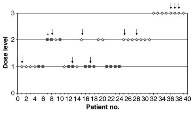
Dose escalation according to the CRM for the example in Geoerger et al (2005). Patients in cohort A (open diamond) and cohort B (closed square) were treated at the dose levels indicated. Arrows indicate observed DLTs, * indicates that the patient was not evaluable for toxicity and was excluded from the CRM. Reprinted from Reference [2].
Table 6.
MTD Recommendation and in-trial allocation for scheme V
| Group 1
|
Group 2
|
|||||||||||
|---|---|---|---|---|---|---|---|---|---|---|---|---|
| d1 | d2 | d3 | d4 | d5 | d6 | d1 | d2 | d3 | d4 | d5 | d6 | |
| Scenario A | ||||||||||||
| Group 1 | Group 2 | |||||||||||
| Ratio of N1/N2 = 20/12 | ||||||||||||
| Ri(dk) | .07 | .23 | .31 | .35 | .45 | .57 | .07 | .23 | .31 | .35 | .45 | .57 |
| Prop (di) | 17 | 42 | 26 | 13 | 2 | 0 | 21 | 41 | 31 | 6 | 1 | 0 |
| Prop (pts) | 24 | 27 | 28 | 16 | 5 | 0 | 17 | 40 | 33 | 8 | 1 | 0 |
| Ratio of N1/N2 = 16/16 | ||||||||||||
| Prop (di) | 20 | 35 | 28 | 15 | 3 | 0 | 20 | 45 | 28 | 7 | 1 | 0 |
| Prop (pts) | 25 | 24 | 28 | 17 | 6 | 0 | 18 | 40 | 31 | 9 | 1 | 0 |
| Scenario B | ||||||||||||
| Ratio of N1/N2 = 20/12 | ||||||||||||
| Ri(dk) | .08 | .20 | .35 | .50 | .70 | .80 | .01 | .05 | .18 | .40 | .55 | .70 |
| Prop (di) | 19 | 51 | 28 | 2 | 0 | 0 | 1 | 23 | 68 | 8 | 0 | 0 |
| Prop (pts) | 25 | 35 | 31 | 9 | 5 | 0 | 4 | 33 | 57 | 5 | 0 | 0 |
| Ratio of N1/N2 = 16/16 | ||||||||||||
| Prop (di) | 19 | 49 | 29 | 4 | 0 | 0 | 0 | 18 | 74 | 8 | 0 | 0 |
| Prop (pts) | 26 | 31 | 31 | 10 | 2 | 0 | 3 | 30 | 61 | 7 | 0 | 0 |
| Scenario C | ||||||||||||
| Ratio of N1/N2 = 20/12 | ||||||||||||
| Ri(dk) | .02 | .19 | .31 | .45 | .51 | .63 | .03 | .05 | .11 | .21 | .39 | .50 |
| Prop (di) | 9 | 47 | 39 | 5 | 0 | 0 | 0 | 11 | 60 | 27 | 2 | 0 |
| Prop (pts) | 17 | 32 | 37 | 12 | 3 | 0 | 2 | 21 | 60 | 16 | 0 | 0 |
| Ratio of N1/N2 = 16/16 | ||||||||||||
| Prop (di) | 12 | 42 | 38 | 8 | 1 | 0 | 0 | 8 | 56 | 34 | 3 | 0 |
| 18 | 29 | 37 | 14 | 3 | 0 | 2 | 17 | 58 | 20 | 2 | 0 | |
Acknowledgments
The authors would like to acknowledge the computing assistance of Jianfen Shu on an earlier version of this and the reviewers for many and detailed comments that enabled us to obtain a more focused version of the paper. This work was partially supported by National Institute of Health (Grant Number 1R01CA142859).
References
- 1.Chu PL, Lin Y, Shih WJ. Unifying CRM and EWOC designs for phase I cancer clinical trials. Journal of statistical planning and inference. 2009;139(3):1146–63. [Google Scholar]
- 2.Geoerger B, Vassal G, Doz F, O’Quigley J, Wartelle M, Watson AJ, Raquin MA, Frappaz D, Chastagner P, Gentet JC, Rubie H, Couanet D, Geoffray A, Djafari L, Margison GP, Pein F. Dose finding and O6-alkylguanine-DNA alkyltransferase study of cisplatin combined with temozolomide in paediatric solid malignancies. Br J Cancer. 2005;93(5):529–37. doi: 10.1038/sj.bjc.6602740. [DOI] [PMC free article] [PubMed] [Google Scholar]
- 3.Iasonos A, O’Quigley J. Interplay of priors and skeletons in two-stage continual reassessment method. Stat Med. 2012;30,31(30):4321–36. doi: 10.1002/sim.5559. [DOI] [PMC free article] [PubMed] [Google Scholar]
- 4.O’Quigley J, Pepe M, Fisher L. Continual reassessment method: a practical design for Phase I clinical trials in cancer. Biometrics. 1990;46:33–48. [PubMed] [Google Scholar]
- 5.O’Quigley J, Shen LZ. Continual Reassessment Method: A likelihood approach. Biometrics. 1996;52:163–174. [PubMed] [Google Scholar]
- 6.O’Quigley J, Reiner E. A stopping rule for the continual reassessment method. Biometrika. 1998;85:741–48. [Google Scholar]
- 7.O’Quigley J, Shen L, Gamst A. Two-sample continual reassessment method. Journal of Biopharmaceutical Statistics. 1999;9(1):17–44. doi: 10.1081/BIP-100100998. [DOI] [PubMed] [Google Scholar]
- 8.O’Quigley J. Theoretical study of the continual reassessment method. J Statist Plann Inference. 2006;136:1765–1780. [Google Scholar]
- 9.Piantadosi S, Liu G. Improved designs for dose escalation studies using pharmacokinetic measurements. Stat in Med. 1996;15:1605–18. doi: 10.1002/(SICI)1097-0258(19960815)15:15<1605::AID-SIM325>3.0.CO;2-2. [DOI] [PubMed] [Google Scholar]
- 10.Robbins H, Monro S. A stochastic approximation method. Annals of Math Statist. 1951;29:351–56. [Google Scholar]
- 11.Shen LZ, O’Quigley J. Consistency of continual reassessment method in dose finding studies. Biometrika. 1996;83:395–406. [Google Scholar]
- 12.Silvapulle MJ. On the existence of maximum likelihood estimators for the binomial response models. JR Stat Soc B. 1981;43(3):310–313. [Google Scholar]
- 13.Storer BE. Encylopedia of Biostatistics. Wiley; New York: 1998. Phase I clinical trials. [Google Scholar]
- 14.Wu CFJ. Efficient sequential designs with binary data. J Amer Statist Assoc. 1985;80:974–984. [Google Scholar]
- 15.Yuan Y, Yin G. Dose-response curve estimation: A semiparametric mixture approach. Biometrics. 2011;67(4):1543–54. doi: 10.1111/j.1541-0420.2011.01620.x. [DOI] [PubMed] [Google Scholar]