Mutational and fitness landscapes of an RNA virus revealed through population sequencing

Abstract

RNA viruses exist as genetically diverse populations¹. It is thought that diversity and genetic structure of viral populations determine the rapid adaptation observed in RNA viruses² and hence their pathogenesis³. However, our understanding of the mechanisms underlying virus evolution has been limited by the inability to accurately describe the genetic structure of virus populations. Next-generation sequencing technologies generate data of sufficient depth to characterize virus populations, but are limited in their utility because most variants are present at very low frequencies and are thus indistinguishable from next-generation sequencing errors. Here we present an approach that reduces next-generation sequencing errors and allows the description of virus populations with unprecedented accuracy. Using this approach, we define the mutation rates of poliovirus and uncover the mutation landscape of the population. Furthermore, by monitoring changes in variant frequencies on serially passaged populations, we determined fitness values for thousands of mutations across the viral genome. Mapping of these fitness values onto three-dimensional structures of viral proteins offers a powerful approach for exploring structure–function relationships and potentially uncovering new functions. To our knowledge, our study provides the first single-nucleotide fitness landscape of an evolving RNA virus and establishes a general experimental platform for studying the genetic changes underlying the evolution of virus populations.

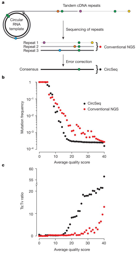
To overcome the limitations of next-generation sequencing error, we developed circular sequencing (CirSeq), wherein circularized genomic RNA fragments are used to generate tandem repeats that then serve as substrates for next-generation sequencing (for DNA adaptation, see ref. 4). The physical linkage of the repeats, generated by ‘rolling circle’ reverse transcription of the circular RNA template, provides sequence redundancy for a genomic fragment derived from a single individual within the virus population (Fig. 1a and Extended Data Fig. 1). Mutations that were originally present in the viral RNA will be shared by all the repeats. Differences within the linked repeats must originate from enzymatic or sequencing errors and can be excluded from the analysis computationally. A consensus generated from a three-repeat tandem reduces the theoretical minimum error probability associated with current Illumina sequencing by up to 8 orders of magnitude, from 10⁻⁴ to 10⁻¹² per base. This accuracy improvement reduces sequencing error to far below the estimated mutation rates of RNA viruses (10⁻⁴ to 10⁻⁶) (ref. 5), allowing capture of a near-complete distribution of mutant frequencies within RNA virus populations.

Figure 1. CirSeq substantially improves data quality.

a, Schematic of the CirSeq concept. Circularized genomic fragments serve as templates for rolling-circle replication, producing tandem repeats. Sequenced repeats are aligned to generate a majority logic consensus (Methods). Green symbols represent true genetic variation. Other coloured symbols represent random sequencing error. NGS, next-generation sequencing. b, c, Comparison of overall mutation frequency (b) and transition:transversion ratio (c) for repeats analysed as three independent sequences (red circles) or as a consensus (black circles). High-quality scores indicate low error probabilities. Quality scores are represented as averages because the consensus quality score is the product of quality scores from each repeat. Data was obtained from a single passage.

We used CirSeq to assess the genetic composition of populations of poliovirus replicating in human cells in culture. Starting from a single viral clone, poliovirus populations were obtained following 7 serial passages (Fig. 2a). At each passage, 10⁶ plaque forming units (p.f.u.) were used to infect HeLa cells at low multiplicity of infection (m.o.i. ∼0.1) for a single replication cycle (8 h) at 37 °C (Methods).

Figure 2. CirSeq reveals the mutational landscape of poliovirus.

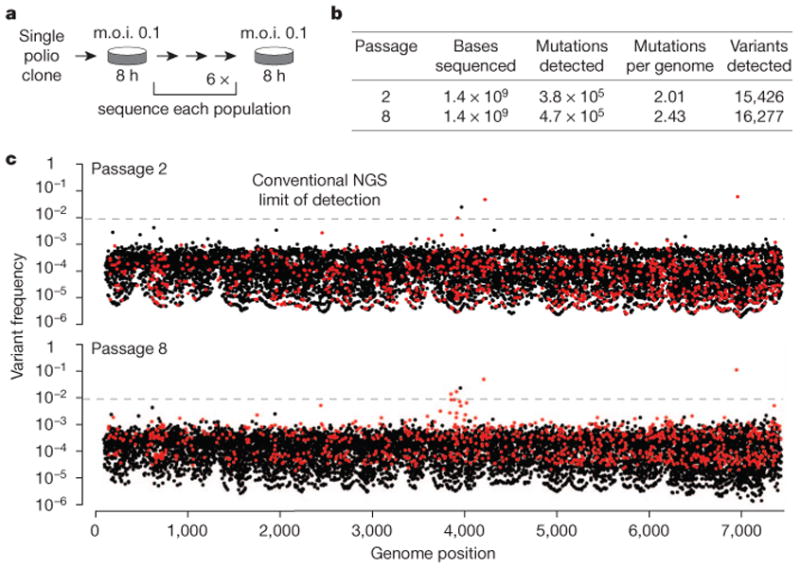
a, Experimental evolution paradigm. A single plaque was isolated, amplified and then serially passaged at low multiplicity of infection (m.o.i.). Low m.o.i. passages were amplified to produce sufficient quantities of RNA for library preparation (Methods). b, Summary of population metrics obtained by CirSeq. c, Frequencies of variants detected using CirSeq are mapped to nucleotide position with the genome for passages 2 and 8. The conventional next-generation sequencing limit of detection (1%) is indicated by dashed lines. Each position contains up to three variants. Variants are coloured based on relative fitness, black indicating lethal or detrimental and red indicating beneficial. Sampling error can affect variant frequencies (see Methods and Extended Data Fig. 4a, b).

We assessed the accuracy of CirSeq relative to conventional next-generation sequencing by estimating overall mutation frequencies as a function of sequence quality (Fig. 1b). The observed mutation frequency using CirSeq analysis was significantly lower than that using conventional analysis of the same data (Fig. 1b). In contrast to conventional next-generation sequencing, the mutation frequency in the CirSeq consensus was constant over a large range of sequencing quality scores (Fig. 1b and Extended Data Fig. 2, quality scores from 20 to 40). The mutation frequency obtained in the stable range of the CirSeq analysis is similar to previously reported mutation frequencies in poliovirus populations—approximately 2 × 10⁻⁴ mutations per nucleotide^3,6 (Fig. 2b and Extended Data Table 1).

We also compared transition-to-transversion ratios (ts:tv) obtained by CirSeq and conventional next-generation sequencing. Although purine (A/G) to purine, or pyrimidine (C/T) to pyrimidine transitions (ts) are the most commonly observed mutations in most organisms⁷, error stemming from Illumina sequencing exhibits substantial purine to pyrimidine or pyrimidine to purine transversion (tv) bias⁸. This bias is reduced using CirSeq, as resulting ts:tv ratios are significantly higher than in the conventional repeat analysis (Fig. 1c). Notably, even if conventional next-generation data are filtered at high sequence quality (that is, quality scores over 30), the ts:tv ratio is still up to 10 times lower than that obtained with CirSeq. Thus, filtering conventional data fails to eliminate most sequencing errors (Fig. 1c). Our results indicate that CirSeq efficiently reduces errors generated during sequencing, producing mutation frequencies and ts:tv ratios consistent with the high values expected for poliovirus^6,9,10.

Using these results, we selected an average quality score of 20 as a threshold for further CirSeq analysis. This threshold corresponds to an estimated error probability of 10⁻⁶ (see Methods), setting a limit of detection for minor genetic variants two orders of magnitude below the expected average mutation frequency for RNA viruses. In comparison, the same quality threshold of 20, generally accepted for conventional analysis of next-generation sequencing data, limits variant detection to a minimum of 1% (ref. 11), two orders of magnitude higher than the average mutation frequency of many RNA viruses.

With an average coverage of more than 200,000 reads per position (Extended Data Fig. 3a), we detected on average more than 16,500 variants, ∼74% of all possible variant alleles, per population per passage (Fig. 2b and Extended Data Table 1). Many alleles were detected for virtually all positions in the genome: mutations for all three alternative alleles (from the remaining three possible alternative nucleotides) were detected at 45.7% of genome positions; mutations for two of three were detected at 42% of positions; and mutations for only one alternative allele were detected at 12.2% of positions. The vast majority of variants are homogenously distributed at low frequencies between 10⁻³ and 10⁻⁵, with very few populating the range between 1 and 10⁻³ (Fig. 2c). Thus, we can infer that the structure of a virus population replicating in the stable environment used here, is characterized by a sharp peak, representing the population consensus sequence, surrounded by a dense array of diverse variants present at very low frequencies (Extended Data Fig. 5a).

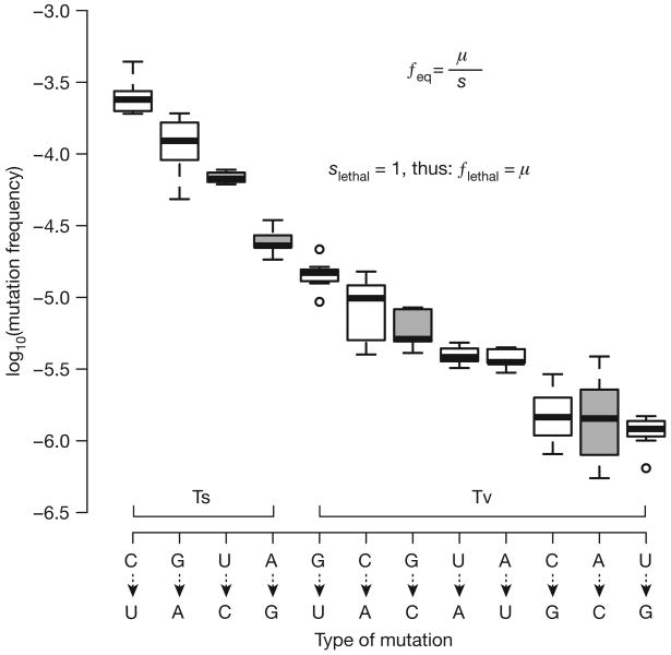
Mutation rates are central to evolution, as the rate of evolution is determined by the rate at which mutations are introduced into the population^12,13. Determination of virus mutation rates is difficult and often unreliable because accuracy depends on observing rare events⁵. We employed CirSeq to measure the rates for each type of mutation occurring during poliovirus replication in vivo. To do so, we estimated the frequency of lethal mutations, which are produced anew in each generation at a frequency equal to the mutation rate¹⁴. These included mutations producing stop codons within the virus polyprotein or those causing amino acid substitutions at catalytic sites of the essential viral enzymes 2A, 3C and 3D^15–17. We find that mutation rates vary by more than two orders of magnitude depending on mutation type, transitions averaging 2.5 × 10⁻⁵ to 2.6 × 10⁻⁴ substitutions per site and transversions averaging 1.2 × 10⁻⁶ to 1.5 × 10⁻⁵ substitutions per site (Fig. 3). Even within these groups, transitions or transversions, the rates of the various nucleotide changes differ by an order of magnitude (Fig. 3). These nucleotide-specific differences in mutation rate likely reflect the molecular mechanism of viral polymerase fidelity, which may ultimately provide a means for the directionality of evolution. For example, C to U and G to A transitions accumulate up to 10 times faster than U to C and A to G; this inequality may provide a mechanistic basis for Dollo's law of irreversibility¹⁸ because the likelihood of moving in one direction in sequence space is not equivalent to the reverse. Our analysis of mutation rates is consistent with biochemical estimations⁹ and provides a physiological view of how the spectrum of mutation rates contribute to the genetic diversity of virus populations.

Figure 3. Determination of in vivo mutation rates of poliovirus.

a, The frequency of deleterious mutations at mutation–selection balance is the mutation rate (μ) over the deleterious selection coefficient (s), see inset. For lethal mutations, s = 1, thus their frequencies equal the mutation rate. Nonsense mutations and catalytic site substitutions were used to obtain lethal mutation frequencies, and thus mutation rates, for each mutation type. Grey boxes were measured using only catalytic site mutants. n = 7 (biological replicates), whiskers represent the lowest and highest datum within 1.5 inner quartile range of the lower and upper quartile, respectively.

We next measured the fitness of each allele in the population by determining the change in mutation frequency for each variant over the course of seven passages (Fig. 2a). Variant frequency is governed by mutation and selection¹⁹, assuming that our experimental conditions (low m.o.i. and large population size at each passage) minimize genetic drift and complementation. We employed a simple model based on classical population genetics to estimate fitness:

$$\frac{a_t}{A_t}=\frac{a_{t-1}}{A_{t-1}}•w_{\mathit{\text{rel}}}+{\mu }_{t-1}$$ (1)

where a and A are the counts of variant and wild type alleles, respectively, w_rel is the relative fitness of a to A (ratio of growth rates), t is time in generations (infection cycles) and μ is the specific rate of mutation from A to a. We measured proportions of A and a over the seven passages and, using mutation rates we previously determined (Fig. 3), calculated w_rel for mutations across the viral genome. The current length limitations of next-generation sequencing preclude CirSeq from providing direct information about haplotypes. Accordingly, our fitness measurements represent the average relative fitness of the population of haplotypes containing a variant allele compared to the population of haplotypes containing the wild-type allele at that position (see Supplementary Information).

Overall, the distribution of mutational fitness effects we obtained (Fig. 4a) is highly consistent with previous small-scale analyses of RNA viruses^20–22, validating CirSeq as a robust method for large-scale fitness measurement. In our analysis, the non-lethal distribution of mutational fitness effects for synonymous mutations is centred near neutrality (Fig. 4a), reflecting the predominantly neutral effects anticipated for synonymous mutations. In contrast, the distribution of non-lethal mutational fitness effects for non-synonymous mutations encompasses primarily deleterious mutations, consistent with previous findings^21–23.

Figure 4. Fitness landscape defines structure–function relationships.

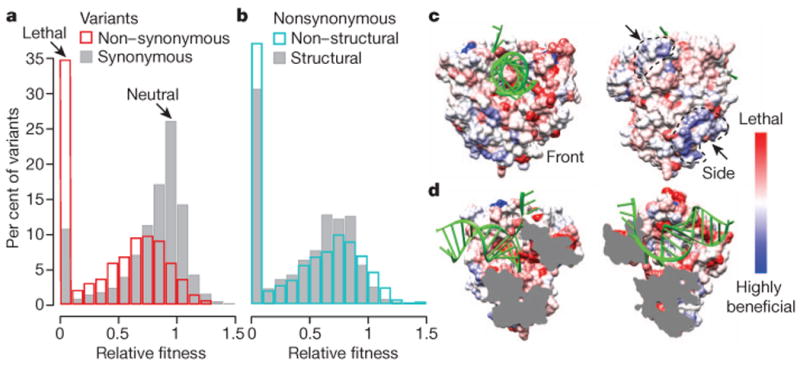
a, b, Distributions of fitness for synonymous (grey) and non-synonymous (red) mutations (a) and for non-synonymous mutations in structural (grey) and non-structural (blue) genes (b). Fitness was determined as described in Methods. C > U and G > A transitions were excluded as we observed indications of hypermutation for these variants. The proportion of lethal variants for each group is likely higher, as not all possible variants were detected. Variants with fitness >1.5 are not shown. c, d, The most fit non-synonymous variant observed for each codon was mapped onto the viral polymerase (3OL6)²⁸ using a red (lethal) to white (neutral) to blue (beneficial) scale. RNA is coloured green. Front and side views show two positively selected surfaces (marked by arrows) (c) and split view shows negative selection along active core and RNA binding sites (d).

Notably, despite the expectation that synonymous mutations will have relatively low impact on fitness, a significant fraction of synonymous changes were subject to strong selection, with 2% being highly beneficial (relative fitness >1.2) and 10% being lethal (Fig. 4a and Extended Data Fig. 6c). Synonymous mutations under strong selection are relatively evenly dispersed throughout the coding sequence, rather than clustered at known functional elements (Extended Data Fig. 6a). Given that the entire capsid-coding region can be deleted without disrupting replication or translation, indicating that this region contains no essential RNA structural elements, it is probable that RNA structure is not the primary driving force behind strong selection of synonymous mutants in poliovirus. Although it is possible that observed mutational fitness effects could be the result of codon usage or codon pair bias, in practice, deoptimization of these biases does not result in lethality based on single nucleotide substitutions^24,25. Future studies will be necessary to elucidate the mechanisms modulated by these synonymous mutations. Furthermore, the variance in fitness for non-synonymous mutations was significantly larger (P < 0.001, Extended Data Fig. 6c) than for synonymous; indeed the largest beneficial fitness effects (not shown in Fig. 4a) were the result of non-synonymous substitutions. Notably, a large number of substitutions are beneficial (145 significantly beneficial mutations, see Methods), indicating the potential for a highly dynamic population structure, where selection for minor genetic components constantly drives the population to new regions of sequence space, even in a relatively constant environment.

The genome-wide distribution of mutational fitness effects does not apply uniformly to each protein as non-synonymous mutations exhibit distinct mutational fitness effects distributions in structural genes (those encoding the viral capsid) and non-structural genes (encoding enzymes and factors involved in viral replication) (Fig. 4b, Extended Data Fig. 6b for synonymous). Although non-structural genes show slightly lower mean mutational fitness effects when considering lethal mutants, they have significantly larger variance in mutational fitness effects (P < 0.001, Extended Data Fig. 6c), indicating that these proteins may have intrinsic differences in their tolerance of mutations. These differences may relate to biophysical properties, like stability constraints²⁶, or the density of functional residues, for example, non-structural proteins often play multifunctional roles and participate in a greater number of host–pathogen interactions²⁷.

To investigate further the relationship between mutational fitness effects and protein structure and function, we mapped fitness values onto the three-dimensional structure of the well characterized poliovirus RNA-dependent RNA polymerase²⁸. We find a remarkable agreement between our fitness data and known structure–function relationships in this enzyme (see Supplementary Information and Extended Data Table 2). For example, many detrimental mutations map to residues associated with RNA binding and catalysis in the central chamber of the polymerase (Fig. 4d, red). Intriguingly, two clusters of beneficial mutations, discontinuous on the genome sequence, mapped to uncharacterized and structurally contiguous regions on the surface of the polymerase (Fig. 4c, blue). Our data suggest that this domain must be functionally relevant to viral replication, as it is clearly tuned by evolution over the course of passaging. Such genome-wide fitness calculations enabled by CirSeq, combined with structural information, can provide high-definition, bias-free insights into structure–function relationships, potentially revealing novel functions for viral proteins and RNA structures, as well as nuanced insights into a viral genome's phenotypic space. Such analyses have the power to reveal protein residues or domains that directly correspond to viral functional plasticity and may significantly inform our structural and mechanistic understanding of host–pathogen interactions.

The analytical approach we describe provides an opportunity to examine and quantify evolutionary dynamics at nucleotide resolution on a genome-wide scale and to integrate evolutionary information with structural and physiological data. Such large-scale measurements of fitness are a fundamental step in understanding the effects of mutation on phenotype and evolutionary trajectory. Modelling the evolutionary dynamics of infection, transmission, host-switching and drug resistance may be central for developing innovative strategies for drug and vaccine design, personalized treatment and the containment of emerging viruses.

Methods

Cells and viruses

HeLa S3 cells (ATCC, CCL2.2) were propagated in DMEM high glucose/F12 medium supplemented with 10% newborn calf serum (Sigma) and 1X penicillin streptomycin glutamine (Gibco) at 37 °C. Wild-type poliovirus type 1 Mahoney was generated by electroporation of cells with T7 in vitro transcribed RNA from linearized prib(+)XpA³¹. A single plaque isolated from this initial population was amplified and Sanger sequenced to ensure the founding clone was wild-type poliovirus. This clone was serially passaged on monolayers containing 10⁷ cells at an m.o.i. of approximately 0.1. To generate populations for sequencing, each passage was amplified on monolayers containing 10⁷ cells at an m.o.i. greater than 5 for 6–8 h. Once a cytopathic effect was observed, the medium was removed and replaced with 2 ml of TRIzol reagent (Ambion).

Library preparation

Total cellular RNA was extracted and precipitated using TRIzol reagent according to the manufacturer guidelines. The RNA was precipitated two times with 0.3 M sodium acetate (pH 5.5) and 2.5 volumes of ethanol before poly(A) selection using the MicroPoly(A)Purist kit (Ambion) according to the manufacturer guidelines. Then 2–5 μg of poly(A)-containing RNA was fragmented with fragmentation reagent (Ambion) for 7.5 min at 70 °C. A practical minimum for this library preparation is 1 μg to ensure that enough fragmented RNA is obtained to produce a library with sufficient complexity and handle reproducibly. Approximately 80–90-base RNA fragments (Extended Data Fig. 3b, for discussion of size) were isolated by 12.5% urea–PAGE and eluted by the crush and soak method. The size-selected RNA was purified from gel fragments using a Spin-X (Costar) cellulose acetate column and ethanol precipitated with glycogen as a carrier. RNA was circularized using polynucleotide kinase and RNA ligase 1 in RNA ligase 1 buffer (NEB) containing 1 mM ATP. Circularized RNA was ethanol precipitated and reverse transcribed with Superscript III (Life Technologies) using the following conditions. First, circularized RNA and 100 ng of random hexamers were combined in a total volume of 10 μl with dNTPs at a final concentration of 2 mM. The reaction was heat denatured at 65 °C for 5 min and then placed on ice for 3 min. Next, 400 U of Superscript III was added as well as dithiothreitol (DTT) to 5 μM and First-Strand Buffer to 1X in a total volume of 20 μl. The reaction was incubated at 25 °C for 10 min, followed by 42 °C for 30 min. After the shift to 42 °C, 0.008 U RNaseH was added to the reaction to allow degradation of the circular form of the RNA. Importantly, Superscript III is a strand-displacing polymerase. As the polymerase transcribes the template, any complementary sequence hybridized downstream of the replication site is displaced by the polymerase allowing transcription of many copies of the same template. In the case of our circular templates, this process results in the polymerase displacing the 5′ end of the nascent strand that it is actively transcribing resulting in multiple copies of the same template on the same nascent strand. After cDNA synthesis, samples were cloned using the following kits consecutively and according to the manufacturer guidelines: NEBNext mRNA Second Strand Synthesis Module (NEB), NEBNext End Repair Module (NEB), NEBNext dA-Tailing Module (NEB) and NEBNext Quick Ligation Module (NEB). Samples were extracted with phenol:chlorofom:isoamyl alcohol (25:24:1 v/v) (Ambion) and precipitated between each reaction. For ligation, oligonucleotides containing Alumina paired-end adaptor sequences (5′-P-GATCGGAAGAGCGGTTCAGC AGGAATGCCGA*G and 5′-ACACTCTTTCCCTACACGACGCTCTTCCGA TC*T, where * indicates a phosphorothioate bond), purchased from IDT, were annealed and used at a final concentration of 2.4 μM. Ligated DNA was size selected from approximately 360–500 bases by 10% urea–PAGE, eluted and precipitated. This purified DNA was then amplified with 1 U Phusion High-Fidelity DNA Polymerase in HF Buffer (NEB) with Primers 1.01 and 2.01 (5′-AATGATA CGGCGACCACCGAGATCTACACTCTTTCCCTACACGACGCTCTTCCGA TC*T and 5′-CAAGCAGAAGACGGCATACGAGATCGGTCTCGGCAT TC CTGCTGAACCGCTCTTCCGATC*T, respectively) at final concentrations of 0.5 μM using the following cycling parameters: 98 °C for 30 s, 15 cycles of 98 °C for 10 s, 65 °C for 30 s, 72 °C for 30 s, followed by 72 °C for 5 min. The amplified library was purified by 5% non-denaturing PAGE. Extended Data Fig. 1 presents a schematic representation of this protocol.

Sequencing and primary data analysis

The 323-cycle single-end sequencing of each library was performed on an Illumina MiSeq. Tandem repeats were identified using an algorithm to define the most common periodicity of subsequences within each read. This was accomplished by looking for the patterns of reoccurrence of substrings within each read. The most common distance between reoccurrences of multiple substrings was set as the periodicity for the read and used to slice the read into individual repeats. These repeats were required to share at least 85% identity in order to accept a consensus, which was generated by majority logic decoding using three repeats.

As each consensus contains information derived from three repeats, the quality of that consensus is determined by the quality of each of those repeats. The quality of each base in each repeat is assessed by base-calling software and given a numerical score, called a quality score. This quality score is a measure of the estimated error probability, or the probability that the base was called incorrectly, according to the following relationship, where Q is the quality score of the base and e is its estimated error probability.

$$Q=-10•{\mathit{\text{log}}}_{10}(e)$$

Because each repeat is an independent observation of the initial genomic template, we can apply the multiplication rule to calculate the estimated error probability of each consensus base. When all three repeat bases are in agreement with the consensus base, the estimated error probabilities derived from each base's quality score can be directly multiplied to obtain the estimated error probability of the consensus base. For example, if all three repeat bases are the same and the quality score for each base is Q20 (e = 10⁻²), the estimated error probability for the consensus base is 10⁻⁶ (10⁻²×10⁻²×10⁻²).

$$e_{\mathit{\text{consensus}}}=e_{\mathit{\text{repeat}}1}•e_{\mathit{\text{repeat}}2}•e_{\mathit{\text{repeat}}3}$$

For bases not in agreement with the consensus, the probability that the true repeat base did not match the consensus was defined as 1 − e/3. For example, if the consensus base was defined as G and the repeat base was read as A, then the probability that the true repeat base was not G is the probability that A was read correctly (1 − e) plus the probability that A was read incorrectly and that the true repeat base was either C or T (2e/3), assuming an equal probability of reading C, G or T.

$$e_{\mathit{\text{Gconsensus}}}=e_{\mathit{\text{Grepeat}}1}•e_{\mathit{\text{Grepeat}}2}•(1-\frac{e_{\mathit{\text{Arepeat}}3}}{3})$$

Once multiplied, these adjusted error probabilities were transformed to quality scores and divided by three to represent an average quality score. The quality scores were averaged to avoid null characters in the ASCII scale used to represent quality scores in FASTQ format.

Consensus sequences along with their corresponding average quality scores were input to Bowtie 2 (ref. 29) using the poliovirus Mahoney strain (accession number V01149) with a single nucleotide substitution U2133C as a reference sequence. Because reverse transcription of circular RNA templates was initiated randomly, the 5′ end of the tandem repeats is not necessarily the 5′ end of the circularized fragment from which they were templated. As a result, most consensus sequences do not align to the reference in their entirety. To accommodate this, all consensus sequences that required soft clipping at one end of the sequence were rearranged by swapping the position of the clipped nucleotides to the opposite end of the sequence. These rearranged sequences were then realigned to the reference. Because mutations, especially those near the fragment ends, can affect alignment and clipping, consensus sequences containing mutations according to their alignment or that required additional clipping after rearrangement were subjected to a more stringent rearrangement algorithm to reduce the chance of introducing artefacts in subsequent analyses. The more stringent rearrangement algorithm optimizes the edit distance of each consensus sequence from the reference by using a repetitive indexing strategy to identify the longest possible seed containing no mutations. This seed was extended base-by-base on either end allowing for the minimum number of mutations and excluding mutations directly at the ends. These rearranged sequences were then run through Bowtie 2 again. Only consensus sequences devoid of indels and clipped bases were used for further analyses to avoid artefacts.

Analysis of mutation frequency

A table of counts of each base at each reference position for each quality score was generated using alignments from the primary analysis. Overall mutation frequencies were calculated for each quality score by dividing the number of mutations called by the total number of bases called for all genome positions for each of the quality scores. Additionally, these frequencies were broken down by transition (purine > purine, pyrimidine > pyrimidine) and transversion (purine > pyrimidine, pyrimidine > purine) mutations for each quality score.

Analysis of the relationship between average quality score and mutation frequency shows that, overall, mutation frequency is stable between Q20 and Q40 (Fig. 1b). This indicates that the frequencies obtained by CircSeq are at or approaching the correct population average mutation frequency over this range. A steep increase followed by a plateau of the transition:transversion (ts:tv) ratio is observed over this same interval (Fig. 1c), indicating that ts:tv ratios obtained by CircSeq are at or approaching the true population ts:tv ratio. One noticeable difference in these measures is the tiered plateau of the ts:tv ratio. This tiered plateau is the result of a tiered plateau of mutation frequencies for transversions (Extended Data Fig. 2). The reason for this tiering is that each type of mutation plateaus at a different level based mostly on its mutation rate. Before the mutation type with the lowest mutation rate levels off, small amounts of error can contribute to an increased mutation frequency for all of the mutation types as a group. This is the effect seen in the upper tier of the transversions. The result of this effect is less apparent in the total mutation frequency where transversions are a much smaller proportion of the total mutations; however, the ts:tv ratio is much more sensitive to small changes in the transversion frequency. All further analyses were carried out with data filtered for a minimum average quality score of 20, because this analysis revealed Q20 to be generally reliable. Quality can be improved further, especially for ultra-rare variants (frequency <10⁻⁶), by shifting this threshold to higher quality scores, however, a higher threshold will result in greater loss of data quantity. A summary of the final sequencing output threshold at Q20 can be found in Extended Data Table 1.

Although the measurement accuracy of the overall mutation frequency for the population is determined by quality scores, the measurement accuracy of individual mutation frequencies at each position of the genome is affected by both the depth of coverage at that position (Extended Data Fig. 3a) and its true mutation frequency. The standard error of a binomial distribution can be used to approximate this error, where n is the coverage depth and p is the mutation frequency measured by sequencing.

$$\mathit{\text{SE}}=\sqrt{\frac{p(1-p)}{n}}$$

Extended Data Fig. 4a demonstrates that lower error estimated by this distribution corresponds to highly correlated frequency measurements from technical replicates. For the technical replicate data sets, this high correlation/low measurement error tends to occur where frequencies are relatively high (∼10⁻⁴ to 10⁻¹). However, even at high frequencies, many variants still have substantial measurement error. Extended Data Fig. 4b shows that this can mainly be explained by coverage, where positions that are covered more deeply also tend to correlate more strongly between replicates. However, the coverage depth required for good correlation increases as frequency decreases, thus coverage must be tailored to the range of frequencies expected for each population.

Random PCR amplification bias (jackpotting) could potentially affect the reliability of mutation frequency measurements. To evaluate this potential source of error, we analysed the distribution of frequencies of nonsense mutations. For the same type of nonsense mutation, their frequency should be at approximately the same frequency (see analysis of mutation rates) in a given passage, but, because there are many of them dispersed throughout the genome, if there is amplification bias (jackpotting), we will likely see at least one instance of uncharacteristically high frequency. Looking at C to U nonsense mutants, which have the highest frequencies and thus give higher quality information, frequencies are clustered around the mean with no large deviations (Extended Data Fig. 4c). This strongly indicates that our experiment is not affected by pervasive jackpotting.

Analysis of mutation rates

The frequencies of lethal mutations were used to estimate the mutation rate of each mutation type¹³. Nonsense mutations and non-synonymous mutations in active site residues of proteins 2A, 3C and 3D^14–16 were used for this purpose. Mutation rates were defined by the number of nonsense or non-synonomous codons caused by each type of mutation divided by the total number of codons sequenced at sites susceptible to those mutations. This was done separately for each mutation type and provides the specific mutation rate for each type of mutation rather than the rate of mutation per site in the genome. The rates measured here are mutation rates per cell infection.

Calculation of relative fitness

Lethal fitness was assigned to a variant if for all seven passages its frequency was either less than or equal to the highest measured frequency of a catalytic site mutant of the same type or, because in some cases no mutations were detected, if coverage at positions having no mutations was at least three times the inverse of the highest measured frequency of a catalytic site mutant of the same type. It is possible that some variants defined as lethal using this criterion may be at a frequency slightly higher than the mutation rate, however, the likelihood of this misclassification is reduced because each variant must meet this requirement seven times. The stringency of this criterion may need to be adjusted for experiments using fewer time steps. Fitness for all other variants with at least one mutation per passage was calculated as described below.

The relative fitness of a mutation can be described by a linear model with two parameters for proportions of a mutation across serial passages:

$$\frac{a_t}{A_t}=\frac{a_{t-1}}{A_{t-1}}•w_{\mathit{\text{rel}}}+{\mu }_{t-1}$$ (1)

where a and A are the counts of a mutated and wild-type alleles, respectively, in passages t and t − 1, measured via sequencing, μ_t−1 is the estimated mutation rate for the specific mutation type in passage t − 1, and an unknown parameter w_rel is the relative fitness of the given mutation, which is assumed to be the same for all passages. Because our measurements of allele frequencies have error (Extended Data Fig. 4), especially at low mutation frequencies, we employed a Bayesian autoregression approach to provide a more accurate estimation of fitness with credibility intervals. We further incorporated the stochastic effect of genetic drift in our calculations by simulating random fluctuation in variant frequencies. This approach provides a more realistic estimation of error in our fitness calculations.

Since a finite number of virions (10⁶) are transferred from one passage to the next, the number of mutant viruses in this sample is subject to genetic drift such that b_t−1 is binomially distributed from 0 to 10⁶ with parameter $p=\frac{a_{t-1}}{A_{t-1}}$.

Equation (1) can be rewritten as:

$$\frac{a_t}{A_t}=w_{\mathit{\text{rel}}}•\frac{b_{t-1}}{{10}^6}+{\mu }_{t-1}$$

or

$$\frac{a_t}{A_t}•{10}^6=w_{\mathit{\text{rel}}}•b_{t-1}+{\mu }_{t-1}•{10}^6$$

or

$$\frac{a_t}{A_t}•{10}^6-{\mu }_{t-1}•{10}^6=w_{\mathit{\text{rel}}}•b_{t-1}$$ (2)

From equation (2) we will get:

$$a_t^{″}={10}^6•\left(\frac{a_t}{A_t}-{\mu }_{t-1}\right)=w_{\mathit{\text{rel}}}•b_{t-1}$$ (3)

$$a_t^{″}=w_{\mathit{\text{rel}}}•b_{t-1}$$ (4)

The number mutations $a_t^{″}$ (total number of normalized mutations minus the number of expected random mutation in 10⁶ genomes) should follow a Poisson distribution with unknown parameter λ_t−1 that is defined by simulated counts b_t−1 based on the mutation frequency from the previous passage, and the fitness parameter, w_rel:

$${\lambda }_{t-1}(w_{\mathit{\text{rel}}})=w_{\mathit{\text{rel}}}•b_{t-1}$$

where b_t−1 is simulated from a binomial distribution $B(\frac{a_t}{A_t},{10}^6)$.

The direct maximum likelihood estimation of w_rel using a product of the Poisson likelihood functions for each passage:

$${\text{arg max}}_{w_{\mathit{\text{re}}}l}{\displaystyle \prod _{t=2}^n\frac{{\lambda }_{t-1}{(w_{\mathit{\text{rel}}})}^{a_t^{″}}}{a_t^{″}!}•e_{t-1}^{-\lambda (w_{\mathit{\text{rel}}})}}$$

interprets passages as independent experiments. This is inaccurate because the passages are chain-dependent.

We applied a generalized Bayesian autoregression approach^32,33 to more accurately estimate w_rel. In the initial step, an estimation of relative fitness, ŵ_rel0, is calculated by a simple regression:

$${\widehat{w}}_{{\mathit{\text{rel}}}_0}=\frac{{\displaystyle {\sum }_{t=2}^n(a_t^{″}•b_{t-1})}}{{\displaystyle {\sum }_{t=2}^n{\left(b_{t-1}\right)}^2}}$$

This estimation is also inaccurate because, in order to be the maximum likelihood estimation, it assumes that values of $a_t^{″}$ are taken from normal distributions, when in fact, they are taken from Poisson distributions with λ_t−1(w_rel) parameters. The Bayesian improvement of this ŵ_rel0 estimation is as follows. Let us approximate counts of ‘selected’ mutations, $a_t^{″}$, by normally distributed z_t values with variances ${\sigma }_t^2$. The distributions of z_t depend on parameters λ_t−1(w_rel) and the likelihood function of z_t approximates the likelihood function of $a_t^{″}$ in the neighbourhood of λ_t−1(ŵ_rel0)—the previous parameter estimation. Thus, the log-likelihood function for $a_t^{″}$:

$$L(a_t^{″}|{\lambda }_{t-1}(w_{\mathit{\text{rel}}}))=\text{log}(\frac{1}{a_t^{″}!}•{\lambda }_{t-1}{(w_{\mathit{\text{rel}}})}^{a_t^{″}}•e^{-{\lambda }_{t-1}(w_{\mathit{\text{rel}}})})$$

is approximated by the log-likelihood function for z_t:

$$M(z_t|{\lambda }_{t-1}(w_{\mathit{\text{rel}}}))\approx \frac{1}{2{\sigma }_t^2}{(z_t-{\lambda }_{t-1}(w_{\mathit{\text{rel}}}))}^2+C$$

in a neighbourhood of λ_t−1(ŵ_rel0). Equalizing term-to-term for the two first terms of a Taylor series representation of the $L(a_t^{″}|{\lambda }_{t-1}(w_{\mathit{\text{rel}}}))$ and M(z_t|λ_t−1(w_rel)) log-likelihood functions in the neighbourhood of λ_t−1(ŵ_rel0), we get the following equations for z_t values and their variances ${\sigma }_t^2$:

$$z_t={\lambda }_{t-1}({\widehat{w}}_{{\mathit{\text{rel}}}_0})-\frac{{\widehat{L}}_t^{\prime }}{{\widehat{L}}_t^{″}}$$

$${\mathrm{\sigma }}_t^2=-\frac{1}{{\widehat{L}}_t^{″}}$$

where $L_t^{\prime }=\frac{dL(a_t^{″}|{\lambda }_{t-1}(w_{\mathit{\text{rel}}}))}{d{\lambda }_{t-1}(w_{\mathit{\text{rel}}})}$ and $L_t^{″}=\frac{d^{2}L(a_t^{″}|{\lambda }_{t-1}(w_{\mathit{\text{rel}}}))}{d{({\lambda }_{t-1}(w_{\mathit{\text{rel}}}))}^2}$ are first and second derivatives with their estimations calculated at ŵ_rel0. Indeed, denoting λ_t−1(ŵ_rel0) as λ and taking derivatives of L and M with respect to λ, we get:

$$\frac{dL}{d\lambda }=a_t^{″}•\frac{1}{\lambda }-1$$

$$\frac{d^{2}L}{d{\lambda }^2}=-\frac{a_t^{″}}{{\lambda }^2}$$

$$\frac{dM}{d\lambda }=\frac{-1}{{\sigma }_t^2}(\lambda -z_t)$$

$$\frac{d^{2}M}{d{\lambda }^2}=\frac{-1}{{\sigma }_t^2}$$

From $\frac{d^{2}L}{d{\lambda }^2}=\frac{d^{2}M}{d{\lambda }^2}$ follows $\frac{d^{2}L}{d{\lambda }^2}=\frac{-1}{{\sigma }_t^2}$ or ${\sigma }_t^2=\frac{-1}{\frac{d^{2}L}{d{\lambda }^2}}$

From $\frac{dL}{d\lambda }=\frac{dM}{d\lambda }$ follows $\frac{dL}{d\lambda }=\frac{-1}{{\sigma }_t^2}(\lambda -z_t)=\frac{d^{2}L}{d{\lambda }^2}(\lambda -z_t)$

Therefore, $z_t-\lambda =-\frac{\frac{dL}{d\lambda }}{\frac{d^{2}L}{d{\lambda }^2}}$ or $z_t=\lambda -\frac{\frac{dL}{d\lambda }}{\frac{d^{2}L}{d{\lambda }^2}}$

where, according to the Taylor series rules, the first and second derivatives of L with respect to λ are taken at the λ_t−1(ŵ_rel0) point. The final step is to obtain a new autoregression estimation of w_rel by the weighted least square procedure:

$$\begin{array}{c}\text{matrix of inverse variances}{z}_t:V=\mathit{\text{diag}}(-{\widehat{L}}_t^{″})\\ {\widehat{w}}_{{\mathit{\text{rel}}}_1}={\left(X^T•V•X\right)}^{-1}•X^T•V•z\\ \mathit{\text{Var}}({\widehat{w}}_{{\mathit{\text{rel}}}_1})=\mathit{\text{diag}}\left[{\left(X^T•V•X\right)}^{-1}\right]\end{array}$$

where X^T = {b₁…,b_n−1} and z^T = {z₂,…,z_n}. As a result, we obtained a better autoregression estimation, ŵ_rel1, and its interval of credibility for every simulation of random variable b₁…,b_n−1. 1,000 simulations were estimated for each variant. To prevent negative values of fitness, if μ_t−1 is larger than $\frac{a_t}{A_t}$, then $a_t^{″}$ is set to 1.

To mitigate error in frequency measurements and the effects of random genetic drift, we use multiple serial passages to calculate fitness. The larger the number of serial passages sampled, the more accurate the fitness data will become. Extended Data Fig. 7 shows how increasing the number of passages increases the accuracy of fitness determination. However, a potential pitfall of using a larger number of serial passages is that fitness may change over time as a result of the accumulation of mutations and the emergence of epistatic interactions within the population. To balance the need to obtain accurate fitness values with the need to avoid the impact of long-term evolution, we have sampled the population within a moderate window of time, 7 passages.

Determination of significantly beneficial mutations

Of 8,970 relative fitnesses determined as described above, 944 were greater than 1, that is, were beneficial. However, because many of these values are very close to 1, to be more rigorous, we have calculated the number of these that significantly deviate from neutrality (relative fitness = 1). Taking into consideration the fact that our fitness estimations have posterior t-test distributions, we centralized this distribution by deducting the theoretically expected mean equal to 1, and normalized the distribution by the estimated standard deviation obtained from the distribution of the 1,000 simulated values of w_rel for each position. P values were calculated for every mutation with beneficial fitness. For every given P value, P, the false discovery rate (FDR)³⁴ value was calculated as a P-expected portion of randomly selected positions in the interval of the sorted P value list of positions: from the smallest P value down to P. Based on an FDR of 5%, we found that there are 145 significantly beneficial mutations (P value threshold P < 0.00072).

Drift simulation

Populations of 10⁶ genomes were created for the initial mutation frequencies of 10⁻³, 10⁻⁴, 10⁻⁵ and 10⁻⁶. In each population, the number of existing mutants was multiplied by its relative fitness to get a new number of mutants. Additionally, each wild-type genome was randomly mutagenized with a probability equal to the mutation rate (same as the initial frequency of the mutation) to get an additional set of mutants. The total number of mutants resulting from mutation and selection were combined with the remaining wild-type genomes to compose the replicated population. This population was randomly sampled with replacement 10⁶ times to recapitulate the bottleneck imposed in our experiment. This sampled population then repeated this mutation-selection-drift process to simulate changes in mutation frequencies that could be expected over the course of 7 passages. This simulation was run 1,000 times for each initial frequency and relative fitness (Extended Data Fig. 8, top row). A simple regression of our mutation-selection model for fitness, equation (1), was used to calculate the relative fitness for each simulation (Extended Data Fig. 8, distributions of relative fitness).

Haplotype simulation

The structure of haplotypes in the sequenced populations was simulated by first determining the frequency of each mutation in each passage and normalizing that frequency by multiplying by 10⁶, yielding the total number of each mutation in a population of 10⁶ genomes (equivalent to the bottleneck size in our experiment). The total normalized number of mutations in the first passage was randomly distributed between 10⁶ genomes. Each mutation was classified as either lethal or non-lethal based on calculations of fitness (above) and the total proportion of lethal mutations was determined (generally 40–50% of the total). The number of genomes containing 0, 1, 2, etc. mutations were then reduced by the probability of a genome containing a lethal mutation. For example, genomes with a single mutation had a probability of 0.4 to 0.5 of containing a lethal mutant and genomes with two mutations had a probability of 0.64 to 0.75 of containing a lethal mutant. From the remaining genomes containing non-lethal mutations, a population of 10⁶ genomes was sampled to carry on to the next passage (generation). This population is shown in Extended Data Fig. 5a as passage 2. In subsequent generations, the total number of mutations in the population from the previous generation were tabulated and subtracted from the total normalized number of non-lethal mutants in the current generation. We considered these pre-existing mutations, thus they should not be reintroduced into the current generation. After removing these pre-existing non-lethal mutants from the total normalized mutants, we randomly distributed the remaining de novo mutations between a new set of 10⁶ genomes. The number of genomes containing different numbers of de novo mutations were then reduced by the probability of a genome containing a lethal mutation, which was defined by the proportion of lethal mutants in the total de novo mutants. To combine the pre-existing mutations from the previous generation and the non-lethal de novo mutations from current generation, a randomly chosen genome from the current generation was added to each genome in the population from the previous generation. This produced a population of 10⁶ genomes containing only non-lethal mutants both pre-existing and de novo (Extended Data Fig. 5a) that could be carried on to the next generation.

Mutation accumulation

To analyse the rate of accumulation of selected mutations, we counted the number of times each reference position was read and multiplied by each of the three mutation rates applicable to that site. For example, the number of bases read at a reference position coded by an A was multiplied by the mutation rates of A > C, A > G and A > T to obtain the number of de novo mutations expected at that site. These de novo expectations can be summed across the genome to obtain the total number of de novo mutations expected in each passage. This number was subtracted from the total number of mutations detected in the passage and divided by the total number of bases sequenced to obtain the frequency of mutations accumulated by selection in each passage (Extended Data Fig. 5b). The rate of accumulation of mutations by selection is approximately linear, meaning that, overall, selection is constant over the course of the experiment.

Extended Data

Extended Data Figure 1. CirSeq library preparation scheme.

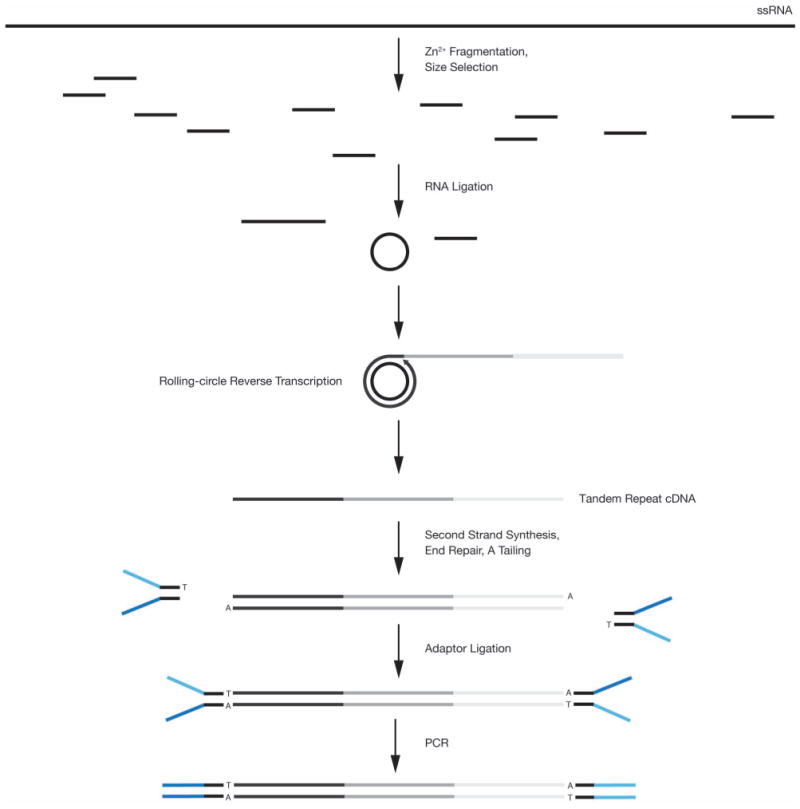
As described in Methods, purified populations of ssRNA viral RNA genomes are converted by a series of molecular cloning steps to a library compatible with Illumina sequencing. Illumina paired-end Y-adaptors are represented in blue.

Extended Data Figure 2. Mutation frequencies of transitions and transversions.

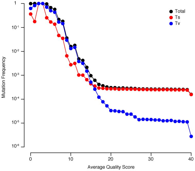
Because transitions (Ts) and transversion (Tv) occur at different rates, the overall frequencies of these types of mutations stabilize at different levels. The lower the mutation frequency, the longer it takes to stabilize, because smaller quantities of error can more dramatically impact their measured frequency. An important consideration for CirSeq is at what quality score to threshold data in order to minimize the contribution of error in the final output and maximize the total quantity of the data used.

Extended Data Figure 3. Genome coverage per base.

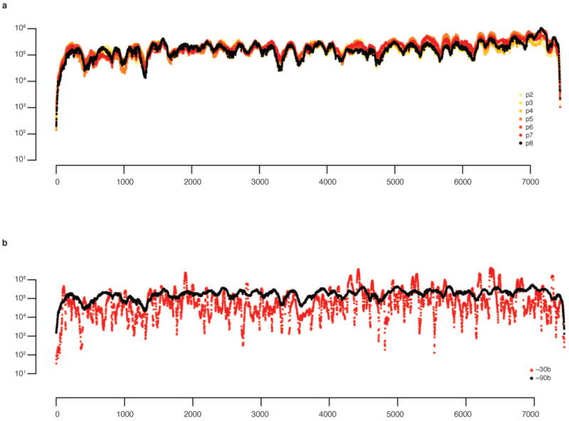
a, Coverage for sequenced passages. The coverage for each base for each library above the minimum quality threshold of average Q20 was mapped. On average, we obtained 204,205-fold coverage for our populations. The coverage profile is extremely consistent between libraries and experiments. b, Effect of RNA fragment size oncoverage bias. Use of fragments less than 80–90 bases in length results in over-representation of A-rich sequences. This bias is likely the result of inefficient priming of certain short templates by reverse transcriptase. Fragments should be at least 80–90 bases, which limits coverage bias to within approximately 10X, typical of RNA-seq.

Extended Data Figure 4. Frequency measurement error.

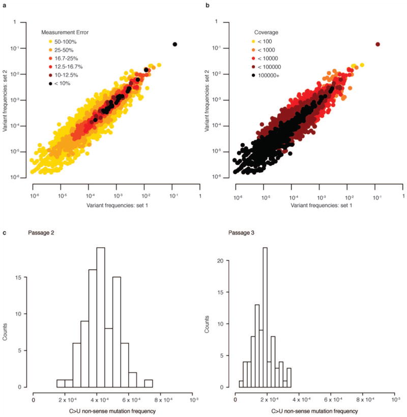
a, b, Error in measurement of mutation frequencies is determined by coverage depth and mutation frequency. A library prepared from 30 base fragments, which increases variability in the level of coverage (see Extended Data Fig. 3b) over different regions of the poliovirus genome, was broken into 10 million read sets (sets 1 and 2). The frequency of each variant for the two sets was mapped against each other to visualize their correlation. a, Measurement error can be estimated as the standard error of a binomial distribution. Per cent error is obtained by dividing this standard error by the variant frequency. Low measurement error corresponds to high correlation between variant frequencies measured in each set. b, Correlation between measured variant frequencies also corresponds to coverage, where greater coverage increases correlation. The amount of coverage required to obtain good correlation between measurements scales with variant frequency. c, Amplification bias. The distribution of frequencies of nonsense mutations generated by C > U mutation are shown for passages 2 and 3. In each case, frequencies are tightly distributed around the mean, ruling out PCR amplification bias in contributing substantially to measurement error of variant frequencies.

Extended Data Figure 5. Inferred population structure and selection over seven passages.

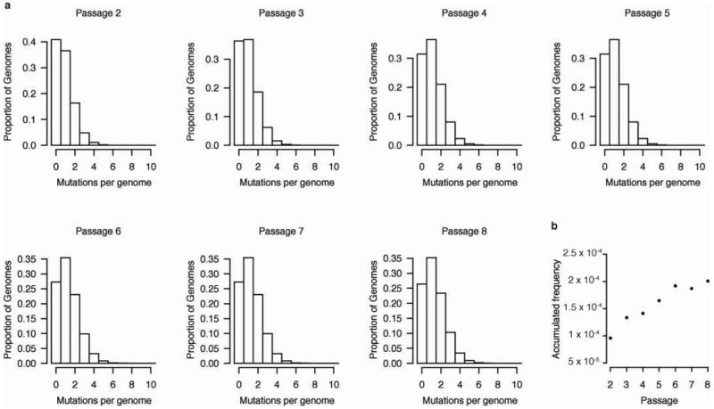
a, Simulation of population structure from sequencing data. The histograms display the proportion of genomes at each passage containing the given number of mutations (Hamming distance from the reference) after removing genomes containing lethal mutations from the population. The proportion of genomes containing single point mutations is relatively constant throughout the passages whereas the proportions of wild-type and multi-variant genomes decrease and increase, respectively. Theses proportions are based on a simulation where mutations are distributed randomly and all viable mutants have fitness equivalent to wild type. b, Accumulation of mutations by selection. The frequency of mutations accumulated as a result of selection, that is, after removing de novo mutations, is plotted for each passage. Mutations accumulate approximately linearly over the course of the experiment suggesting that selection is constant.

Extended Data Figure 6. Analysis of mutational fitness effects.

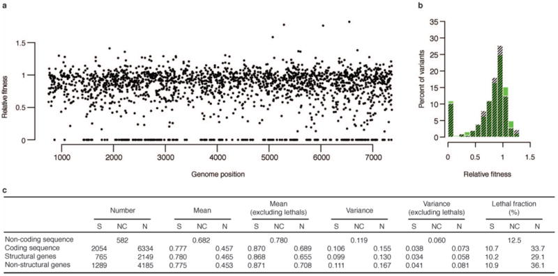
a, Spatial distribution of synonymous mutations by fitness effect. Synonymous mutations were binned by the magnitude of their fitness effect and plotted against their respective genome position. Each bin of fitness effects is well distributed across the genome, indicating that synonymous mutations with strong fitness effects map to discrete regions. b, The distributions of mutational fitness effects of synonymous mutations for structural (black) and non-structural (green) genes are similar. c, Summary of mutational fitness effects. Differences in variance are statistically significant between non-synonymous mutations in structural and non-structural genes both including and excluding lethal mutations (P < 0.001, one-sided F-test). Differences in variance are also statistically significant between non-synonymous and synonymous mutations the coding sequence both including and excluding lethal mutations (P < 0.001, one-sided F-test).

Extended Data Figure 7. Number of passages used to calculate fitness affects accuracy.

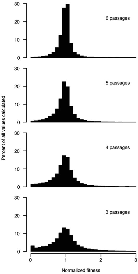
Fitness for each variant was calculated for varying numbers of serial passages and normalized to the fitness calculated using the full set of seven passages. As the number of passages used to calculate fitness increases, the variation in fitness decreases, indicating that the calculated fitness is more accurate.

Extended Data Figure 8. Simulation of genetic drift and its impact on fitness measurement.

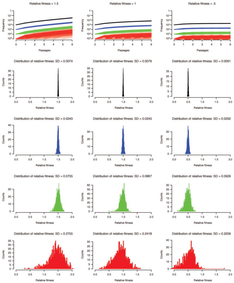
Top row shows one thousand simulations of a mutation-selection-drift process in a population of 10⁶ genomes are shown for mutations initiated at their mutation rate: 10⁻³ (black), 10⁻⁴ (blue), 10⁻⁵ (green) and 10⁻⁶ (red). Because of the low number of mutations in populations where the mutation rate was set to 10⁻⁶, it is common for the population to lose the mutant by drift. As frequency was plotted on alog scale,a frequency of 0 was representedas10⁻⁷. The histograms show fitness calculated using a simple mutation-selection model for each simulation. The standard deviation for each set of calculations is noted in the title of each set of simulations. The stronger drift experienced by low frequency variants reduces the accuracy of fitness measurements. To account for this effect, we have incorporated drift into our fitness model.

Extended Data Table 1. Summary of data collected from sequenced passages.

Passage	Bases sequenced above Q20avg	Mutations detected above Q20avg	Average mutation frequency	Average mutations per genome	Variants detected*	% of alleles detected
2	1,405,927,958	378,993	2.70•10-4	2.01	15426	69.1
3	1,328,448,147	316,931	2.39•10-4	1.77	15780	70.7
4	1,490,238,776	397,442	2.67•10-4	1.98	17259	77.3
5	1,709,503,454	487,695	2.85•10-4	2.12	16778	75.2
6	1,647,601,130	498,477	3.03•10-4	2.25	17631	79.0
7	1,613,382,399	464,184	2.88•10-4	2.15	16670	74.7
8	1,438,501,772	470,689	3.27•10-4	2.43	16277	72.9

Data represented in this table are from consensus sequences filtered at average quality score 20. Variants(*) reported here are statistically significant (P value ≤ 0.05) by an exact binomial test using the average estimated error probability for each site, the coverage and number of mutations detected at each site (for each variant separately).

Extended Data Table 2. Comparison of the phenotypes of published mutants^16,35–39 with fitness calculated using CirSeq.

Protein	Substitution	Fitness (CirSeq)	Phenotype	Reference
2A	H116R	1.00	WT	16
3AB	K9E	0.82	Normal plaques	35
	I12V	1.02	Normal plaques	36
	K39E	0.91	Normal plaques	36
	W42R	0.04	No plaques	36
	V44A	0.87	Normal plaques	36
	N45D	0.94	Normal plaques	36
	I46T	1.02	Normal plaques	36
	L63P	0.65	No plaques	36
	Y77H	0.88	No plaques	36
	K81E	0.88	No plaques	36
	L82P	0.20	No plaques	36
	K107E	0.36	Small plaques	35
3C	K60I	0.70	Small plaques	37
	K60T	0.92	Small plaques	37
	A61E	0	Small plaques	37
	A61V	0.69	Small plaques	37
	A66E	0.74	Small plaques	37
	A66V	0.30	Small plaques	37
	T142I	0.01	Defective viral growth	38
	H161Y	0.07	No in vitro cleavage	38
	G163V	0.56	No in vitro cleavage	38
	A172E	0.46	Impared in vitro cleavage	38
	A172V	0.15	Defective viral growth	38
3D	V33A	0.28	Loss of infectivity	39

References

- 1.Domingo E, Sabo D, Taniguchi T, Weissmann C. Nucleotide sequence heterogeneity of an RNA phage population. Cell. 1978;13:735–744. doi: 10.1016/0092-8674(78)90223-4. [DOI] [PubMed] [Google Scholar]
- 2.Burch CL, Chao L. Evolvability of an RNA virus is determined by its mutational neighbourhood. Nature. 2000;406:625–628. doi: 10.1038/35020564. [DOI] [PubMed] [Google Scholar]
- 3.Vignuzzi M, Stone JK, Arnold JJ, Cameron CE, Andino R. Quasispecies diversity determines pathogenesis through cooperative interactions in a viral population. Nature. 2006;439:344–348. doi: 10.1038/nature04388. [DOI] [PMC free article] [PubMed] [Google Scholar]
- 4.Lou DI, et al. High-throughput DNA sequencing errors are reduced by orders of magnitude using circle sequencing. Proc Natl Acad Sci USA. doi: 10.1073/pnas.1319590110. in the press. [DOI] [PMC free article] [PubMed] [Google Scholar]
- 5.Sanjuán R, Nebot MR, Chirico N, Mansky LM, Belshaw R. Viral mutation rates. J Virol. 2010;84:9733–9748. doi: 10.1128/JVI.00694-10. [DOI] [PMC free article] [PubMed] [Google Scholar]
- 6.Crotty S, Cameron CE, Andino R. RNA virus error catastrophe: direct molecular test by using ribavirin. Proc Natl Acad Sci USA. 2001;98:6895–6900. doi: 10.1073/pnas.111085598. [DOI] [PMC free article] [PubMed] [Google Scholar]
- 7.Wakeley J. The excess of transitions among nucleotide substitutions: new methods of estimating transition bias underscore its significance. Trends Ecol Evol. 1996;11:158–162. doi: 10.1016/0169-5347(96)10009-4. [DOI] [PubMed] [Google Scholar]
- 8.Dohm JC, Lottaz C, Borodina T, Himmelbauer H. Substantial biases in ultra-short read data sets from high-throughput DNAsequencing. Nucleic Acids Res. 2008;36:e105. doi: 10.1093/nar/gkn425. [DOI] [PMC free article] [PubMed] [Google Scholar]
- 9.Freistadt MS, Vaccaro JA, Eberle KE. Biochemical characterization of the fidelity of poliovirus RNA-dependent RNA polymerase. Virol J. 2007;4:44. doi: 10.1186/1743-422X-4-44. [DOI] [PMC free article] [PubMed] [Google Scholar]
- 10.Arnold JJ, Cameron CE. Poliovirus RNA-dependent RNA polymerase (3Dpol): pre-steady-state kinetic analysis of ribonucleotide incorporation in the presence of Mg2+ Biochemistry. 2004;43:5126–5137. doi: 10.1021/bi035212y. [DOI] [PMC free article] [PubMed] [Google Scholar]
- 11.Radford AD, et al. Application of next-generation sequencing technologies in virology. J Gen Virol. 2012;93:1853–1868. doi: 10.1099/vir.0.043182-0. [DOI] [PMC free article] [PubMed] [Google Scholar]
- 12.Orr HA. The rate of adaptation in asexuals. Genetics. 2000;155:961–968. doi: 10.1093/genetics/155.2.961. [DOI] [PMC free article] [PubMed] [Google Scholar]
- 13.Kimura M. The Neutral Theory of Molecular Evolution. Cambridge Univ. Press; 1983. pp. 55–97. [Google Scholar]
- 14.Cuevas JM, González-Candelas F, Moya A, Sanjuán R. Effect of ribavirin on the mutation rate and spectrum of hepatitis C virus in vivo. J Virol. 2009;83:5760–5764. doi: 10.1128/JVI.00201-09. [DOI] [PMC free article] [PubMed] [Google Scholar]
- 15.Hämmerle T, Hellen CU, Wimmer E. Site-directed mutagenesis of the putative catalytic triad of poliovirus 3C proteinase. J Biol Chem. 1991;266:5412–5416. [PubMed] [Google Scholar]
- 16.Hellen CUT, Lee CK, Wimmer E. Determinants of substrate recognition by poliovirus 2A proteinase. J Virol. 1992;66:3330–3338. doi: 10.1128/jvi.66.6.3330-3338.1992. [DOI] [PMC free article] [PubMed] [Google Scholar]
- 17.Gohara DW, et al. Poliovirus RNA-dependent RNA polymerase (3Dpol): structural, biochemical, and biological analysis of conserved structural motifs A and B. J Biol Chem. 2000;275:25523–25532. doi: 10.1074/jbc.M002671200. [DOI] [PubMed] [Google Scholar]
- 18.Gould SJ. Dollo on Dollo's law: irreversibility and the status of evolutionary laws. J Hist Biol. 1970;3:189–212. doi: 10.1007/BF00137351. [DOI] [PubMed] [Google Scholar]
- 19.Haldane JBS. A mathematical theory of natural and artificial selection, part V: selection and mutation. Math Proc Camb Philos Soc. 1927;23:838–844. [Google Scholar]
- 20.Cuevas JM, Domingo-Calap P, Sanjuán R. The fitness effects of synonymous mutations in DNA and RNA viruses. Mol Biol Evol. 2012;29:17–20. doi: 10.1093/molbev/msr179. [DOI] [PubMed] [Google Scholar]
- 21.Eyre-Walker A, Keightley PD. The distribution of fitness effects of new mutations. Nature Rev Genet. 2007;8:610–618. doi: 10.1038/nrg2146. [DOI] [PubMed] [Google Scholar]
- 22.Sanjuán R, Moya A, Elena SF. The distribution of fitness effects caused by single-nucleotide substitutions in an RNA virus. Proc Natl Acad Sci USA. 2004;101:8396–8401. doi: 10.1073/pnas.0400146101. [DOI] [PMC free article] [PubMed] [Google Scholar]
- 23.Chao L. Fitness of RNA virus decreased by Muller's ratchet. Nature. 1990;348:454–455. doi: 10.1038/348454a0. [DOI] [PubMed] [Google Scholar]
- 24.Mueller S, Papamichail D, Coleman JR, Skiena S, Wimmer E. Reduction of the rate of poliovirus protein synthesis through large-scale codon deoptimization causes attenuation of viral virulence by lowering specific infectivity. J Virol. 2006;80:9687–9696. doi: 10.1128/JVI.00738-06. [DOI] [PMC free article] [PubMed] [Google Scholar]
- 25.Coleman JR, et al. Virus attenuation by genome-scale changes in codon pair bias. Science. 2008;320:1784–1787. doi: 10.1126/science.1155761. [DOI] [PMC free article] [PubMed] [Google Scholar]
- 26.Tokuriki N, Tawfik D. Protein dynamism and evolvability. Science. 2009;324:203–207. doi: 10.1126/science.1169375. [DOI] [PubMed] [Google Scholar]
- 27.Jäger S, et al. Global landscape of HIV–human protein complexes. Nature. 2012;481:365–370. doi: 10.1038/nature10719. [DOI] [PMC free article] [PubMed] [Google Scholar]
- 28.Gong P, Peersen OB. Structural basis for active site closure by the poliovirus RNA-dependent RNA polymerase. Proc Natl Acad Sci USA. 2010;107:22505–22510. doi: 10.1073/pnas.1007626107. [DOI] [PMC free article] [PubMed] [Google Scholar]
- 29.Langmead B, Salzberg SL. Fast gapped-read alignment with Bowtie 2. Nature Methods. 2012;9:357–359. doi: 10.1038/nmeth.1923. [DOI] [PMC free article] [PubMed] [Google Scholar]
- 30.Pettersen EF, et al. UCSF Chimera–a visualization system for exploratory research and analysis. J Comput Chem. 2004;25:1605–1612. doi: 10.1002/jcc.20084. [DOI] [PubMed] [Google Scholar]
- 31.Herold J, Andino R. Poliovirus requires a precise 5′ end for efficient positive-strand RNA synthesis. J Virol. 2000;74:6394–6400. doi: 10.1128/jvi.74.14.6394-6400.2000. [DOI] [PMC free article] [PubMed] [Google Scholar]
- 32.Draper NR, Smith H. Applied Regression Analysis. Wiley; 1998. [Google Scholar]
- 33.Gelman A, Carlin JB, Stern HS, Rubin DB. Bayesian Data Analysis. Chapman & Hall/CRC Texts in Statistical Science; 2003. [Google Scholar]
- 34.Benjamini Y, Hochberg Y. Controlling the false discovery rate: a practical and powerful approach to multiple testing. J R Stat Soc B. 1995;57:289–300. [Google Scholar]
- 35.Lama J, Sanz MA, Rodríguez PL. A role for 3AB protein in poliovirus genome replication. J Biol Chem. 1995;270:14430–14438. doi: 10.1074/jbc.270.24.14430. [DOI] [PubMed] [Google Scholar]
- 36.Lama J, Sanz MA, Carrasco L. Genetic analysis of poliovirus protein 3A: characterization of a non-cytopathic mutant virus defective in killing Vera cells. J Gen Virol. 1998;79:1911–1921. doi: 10.1099/0022-1317-79-8-1911. [DOI] [PubMed] [Google Scholar]
- 37.Dewalt PG, Blair WS, Semler BL. A genetic locus in mutant poliovirus genomes involved in overproduction of RNA polymerase and 3C proteinase. Virology. 1990;174:504–514. doi: 10.1016/0042-6822(90)90104-y. [DOI] [PubMed] [Google Scholar]
- 38.Blair WS, Nguyen JHC, Parsley TB, Semler BL. Mutations in the poliovirus 3CD proteinase S1-specificity pocket affect substrate recognition and RNA binding. Virology. 1996;218:1–13. doi: 10.1006/viro.1996.0160. [DOI] [PubMed] [Google Scholar]
- 39.Hobson SD, et al. Oligomeric structures of poliovirus polymerase are important for function. EMBO J. 2001;20:1153–1163. doi: 10.1093/emboj/20.5.1153. [DOI] [PMC free article] [PubMed] [Google Scholar]
Associated Data
This section collects any data citations, data availability statements, or supplementary materials included in this article.