Parallel continuous simulated tempering and its applications in large-scale molecular simulations

Abstract

In this paper, we introduce a parallel continuous simulated tempering (PCST) method for enhanced sampling in studying large complex systems. It mainly inherits the continuous simulated tempering (CST) method in our previous studies [C. Zhang and J. Ma, J. Chem. Phys. 141, 194112 (2009); C. Zhang and J. Ma, J. Chem. Phys. 141, 244101 (2010)], while adopts the spirit of parallel tempering (PT), or replica exchange method, by employing multiple copies with different temperature distributions. Differing from conventional PT methods, despite the large stride of total temperature range, the PCST method requires very few copies of simulations, typically 2–3 copies, yet it is still capable of maintaining a high rate of exchange between neighboring copies. Furthermore, in PCST method, the size of the system does not dramatically affect the number of copy needed because the exchange rate is independent of total potential energy, thus providing an enormous advantage over conventional PT methods in studying very large systems. The sampling efficiency of PCST was tested in two-dimensional Ising model, Lennard-Jones liquid and all-atom folding simulation of a small globular protein trp-cage in explicit solvent. The results demonstrate that the PCST method significantly improves sampling efficiency compared with other methods and it is particularly effective in simulating systems with long relaxation time or correlation time. We expect the PCST method to be a good alternative to parallel tempering methods in simulating large systems such as phase transition and dynamics of macromolecules in explicit solvent.

I. INTRODUCTION

The main objective of computer simulation in equilibrium statistical physics is to calculate the ensemble average of interested physical properties ⟨A⟩ (for example, average potential energy ⟨E⟩ and mean square fluctuation ⟨(ΔE)²⟩, which is related to heat capacity C_V). The simulation in canonical ensemble can sample the phase space at constant temperature, but the system is easy to get trapped in local minima for a long time.¹ This phenomenon is called broken ergodcity and it limits the accuracy of computed physical properties with trajectories of finite length.

During the past decades, generalized ensemble² was introduced to overcome the broken ergodcity issue. As its name implies, a generalized ensemble uses a more general form of probability distribution W(X, β) instead of the Boltzmann distribution P_Boltz(X; β) = Z(β)⁻¹e^−βE(X), where X is the configuration, β is the reciprocal temperature, E(X) is the potential energy, and Z(β) is the canonical partition function. Among all the generalized ensembles, the idea of multicanonical ensemble^3,4 has been widely used because of its high barrier-crossing efficiency in the configurational space (CS). The multicanonical ensemble generates a flat histogram of potential energy and its mathematical form of W(X, β) can be written as W(X)∝Ω⁻¹(E(X)) = e^{−βTS(E(X))}, where Ω(E(X)) represents the density of states, T is the temperature and S(E(X)) represents the microcanonical entropy. Multicanonical ensemble has already been shown to be very effective in the simulation of many complex systems such as the spin glass,^3,5 simple liquid systems,⁶ small peptides,⁷ and structure-based model of proteins.⁸

Another typical approach of generalized ensemble is called simulated tempering (ST),⁹ which generates a flat histogram of temperature, i.e., W(T) = const. or a flat histogram of reciprocal temperature, i.e., W(β) = const. In small peptide simulation, the performance of flat energy histogram method and flat temperature histogram method was shown to be similar.¹⁰ However, a flat histogram in temperature space does not need to estimate Ω(E) or S(E) of the system,^11–13 which makes it easier to be applied to larger systems, such as the protein folding simulation in explicit solvent.¹³ ST is particularly useful in the situation that the energy change upon folding of polypeptide is smaller than the total energy fluctuation of the entire system when a large water box is present. In conventional ST, the system jumps between various discrete temperatures.⁹ Since the acceptance ratio for every attempt of jump is related to the overlap between the energy histograms of two canonical ensembles,¹⁴ it decreases quickly when the system size increases. In our previous studies,^12,13 a single-copy continuous simulated tempering (CST) method was proposed to overcome this limitation and allow the application of ST in larger systems. The CST method has already been shown to be very successful in folding simulation of small proteins in explicit solvent.^13,15 However, for systems with long relaxation time such as folding a long polypeptide¹⁶ or correlation time such as phase transition,¹⁷ a single copy method is often far from enough because the residing time of the simulation in the important temperature range (e.g., near room temperature in folding) is shorter than the relaxation time of the system (the time required for the polypeptide chain to structurally rearrange).

Parallel tempering (PT),^18,19 or replica exchange, provides another way of searching the CS. In PT, multiple copies are used and each copy samples in canonical ensemble at different temperatures. At certain time intervals, an attempt of temperature exchange between neighboring copies is made with the acceptance ratio of min{1, e^ΔβΔE}, where Δβ and ΔE represent the temperature and potential energy difference between involved copies, respectively. In the conventional PT, one of the major limitations in simulating large systems is that the acceptance ratio falls sharply when the system size increases as ΔE becomes quite large.²⁰ To avoid this, an increase of copy $\propto \sqrt{N}$ (N is the degree of freedom)²⁰ is required to keep a reasonable acceptance ratio, which consumes the computing resources significantly. Although progresses²¹ have also been made to increase the exchange probability and extend the scope of PT, this issue remains to be a major obstacle in the application of conventional PT in large systems.

In this paper, we introduce a new method for importance sampling in molecular simulation of large complex systems. This method inherits features from CST method^12,13 in our previous studies and adopts the spirit of PT in employing multiple copies with different temperature distributions and a specific exchange protocol to satisfy the detailed balance. The temperature distribution in each copy is specified in a large temperature range, and the energy histograms are much wider than the ones in canonical ensemble, which brings a sufficient overlap between them and thus guarantees a higher exchange rate. Furthermore, an important feature of our method is that the exchange rate is independent of total potential energy E, therefore it does not suffer from the increasing of copy number with the growth of the system size compared to conventional PT (in practice, typical number of copies is 2–3). With the combination of CST and PT, the PCST method can effectively simulate the systems with long relaxation times or correlation times.

We present the paper as follows: in Sec. II, we first make a review of the CST method^12,13 along with the estimator based on integral identities¹² developed in our previous studies, and then introduce the parallel probability distribution and the exchange protocol in the PCST method. In Sec. III, the performance of the PCST method is demonstrated in three typical systems, the two-dimensional (2D) Ising model, the Lennard-Jones fluid, and small protein folding (trp-cage) simulation in explicit solvent. The significant performance improvement of PCST over CST is clearly demonstrated in folding simulations. In Sec. IV, we make a summary of the results and discuss the perspectives.

II. METHOD

A. Generalized ensemble

To avoid the direct calculation of density of states Ω(E) or microcanonical entropy S(E) for large, complex systems, a generalized ensemble that is a collection of canonical ensembles at different temperatures was proposed in previous study,¹² whose probability distribution function, P(X, β), follows:

$$P\left(X,\beta \right)=C{Z}^{-1}\left(\beta \right)e^{-\beta E\left(X\right)}\omega \left(\beta \right),$$ (1)

where X is the configuration, β is the reciprocal temperature defined in a large range (β_min, β_max), ω(β) is the weight of canonical ensemble at the temperature β in the generalized ensemble, C is the normalization factor of ω(β), E(X) is the potential energy, and Z(β) is the canonical partition function. It was also shown that¹³ a choice of $\omega \left(\beta \right)\propto \sqrt{C_V\left(\beta \right)}/\beta$ would optimize the energy histogram overlap between canonical ensembles at neighboring temperatures. For example, in a system with a roughly constant heat capacity (such as ideal gas or Lennard-Jones system), the optimized ω(β) would be β⁻¹ and for other systems like proteins in which heat capacity was observed as ∝ β, a suggested ω(β) would be β^−1/2. Generally speaking, ω(β) can be represented as β^−γ if $\sqrt{C_V\left(\beta \right)}\propto {\beta }^{1-\gamma }$.

B. Parallel generalized ensemble for importance sampling

There are many cases in which one needs to pay special attention to sampling around an important but narrow temperature range, such as the temperature around the critical temperature T_c in simulation of phase transition. Another example is the protein folding simulation, in which the long simulation around room temperature is needed for more thorough sampling near the native state as the relaxation timescales of polypeptides are quite long for large systems.¹⁶ On the other hand, simply biasing the single copy simulation in generalized ensemble toward the lower temperature is not enough, as this will increase the possibility for the system to be trapped in an energy basin at lower temperature and also decrease the ability of barrier crossing at high temperature. To solve the dilemma between barrier-crossing efficiency and demand of importance sampling around key temperature range, we propose a multiple-copy method with the probability distribution of the revised generalized ensemble as follows:

$$P(X,\beta )=C{Z}^{-1}\left(\beta \right)e^{-\beta E\left(X\right)}{\beta }^{-\gamma }{f}_i\left(\beta \right)$$ (2)

for the ith copy. The function f_i(β) can be designed to either increase or decrease the weight of canonical ensemble at temperature β and the sampling time on certain temperature ranges. For example, a Gaussian function $e^{-{\left(\beta -{\beta }_i^0\right)}^2/2{\sigma }_i^2}$ can focus the importance sampling around the interested temperature ${\beta }_i^0$.

In order to facilitate barrier crossing at high temperature and thorough sampling at lower temperature, we introduce a parameter exchange protocol between high temperature copies and low temperature copies. In this protocol, the acceptance ratio for copy exchange between the ith copy and the jth copy is defined as

$$\begin{array}{ccc}& & Acc\left(X_i{\beta }_i{\beta }_i^0{\sigma }_i,X_j{\beta }_j{\beta }_j^0{\sigma }_j\to X_j{\beta }_j{\beta }_i^0{\sigma }_i,X_i{\beta }_i{\beta }_j^0{\sigma }_j\right)\hfill \\ & & =\min \left\{1,\frac{P\left(X_j,{\beta }_j;{\beta }_i^0,{\sigma }_i\right)P\left(X_i,{\beta }_i;{\beta }_j^0,{\sigma }_j\right)}{P\left(X_i,{\beta }_i;{\beta }_i^0,{\sigma }_i\right)P\left(X_j,{\beta }_j;{\beta }_j^0,{\sigma }_j\right)}\right\}\hfill \\ & & =\min \left\{1,e^{-\left(\Delta \beta \Delta q_0+\Delta {\beta }^2\Delta q_1\right)}\right\},\hfill \end{array}$$ (3)

where Δβ ≡ β_i − β_j, $\Delta {\beta }^2\equiv {\beta }_i^2-{\beta }_j^2$, $\Delta q_0\equiv {\beta }_i^0/{\sigma }_i^2-{\beta }_j^0/{\sigma }_j^2$, and $\Delta q_1\equiv -1/\left(2{\sigma }_i^2\right)+1/\left(2{\sigma }_j^2\right)$.

Specially, if the variances of different distributions are the same, i.e., σ_i = σ_j, then the acceptance ratio becomes

$$\begin{array}{ccc}& & Acc\left(X_i{\beta }_i{\beta }_i^0,X_j{\beta }_j{\beta }_j^0\to X_j{\beta }_j{\beta }_i^0,X_i{\beta }_i{\beta }_j^0\right)\hfill \\ & & =\min \left\{1,\frac{P\left(X_j,{\beta }_j;{\beta }_i^0\right)P\left(X_i,{\beta }_i;{\beta }_j^0\right)}{P\left(X_i,{\beta }_i;{\beta }_i^0\right)P\left(X_j,{\beta }_j;{\beta }_j^0\right)}\right\}\hfill \\ & & =\min \left\{1,e^{-\Delta \beta \Delta {\beta }^0/{\sigma }^2}\right\},\hfill \end{array}$$ (4)

where $\Delta {\beta }^0\equiv {\beta }_i^0-{\beta }_j^0$.

It is easy to show that this protocol satisfies the detailed balance. An important feature of the parameter exchange protocol is that the acceptance ratio is only related to the parameters in generalized ensemble and the current temperature, whereas it does not have an explicit dependence on the current potential energy E. Therefore, compared with the conventional replica-exchange method,¹⁸ this method does not suffer from a decrease of successful exchange rate with the increase of system size. Moreover, the acceptance ratio is user-adjustable via changing the parameters in generalized ensemble. It is noted that at the limit σ → 0, the generalized ensemble is converted into isolated canonical ensembles at temperature ${\beta }_i^0$ for the ith copy. In this case, if the temperature gap Δβ⁰ is relatively large, then the exchange ratio will decrease to zero.

C. Temperature random walk to guild a continuous tempering

In continuous tempering, a temperature random walk scheme is used instead of the acceptance ratio scheme in conventional ST to generate the desired P(X, β). We first write down a general form of one-dimensional Fokker-Planck equation, which follows:

$$\frac{\partial \rho \left(T\right)}{\partial t}=-\frac{\partial }{\partial T}\left[\mu \left(T\right)\rho \left(T\right)\right]+\frac{{\partial }^2}{\partial T^2}\left[D\left(T\right)\rho \left(T\right)\right],$$ (5)

where ρ(T) is the instant temperature probability distribution, D(T) is a diffusion term, and μ(T) represents a drift force in temperature space with the mathematical form of ∂_T[D(T)P(X, T)]/P(X, T) = D(T)∂_T ln P(X, T) + ∂_TD(T). Based on the equivalence of Brownion motion and one-dimensional F-P equation in this case, a temperature space random walk can be written as

$$dT=\left[D\left(T\right)\frac{\partial \ln P\left(X,T\right)}{\partial T}+\frac{\partial D\left(T\right)}{\partial T}\right]dt+\sqrt{2D\left(T\right)}dW,$$ (6)

where dW is the Weiner process. It can be easily shown that the stationary distribution of this F-P equation is P(X, T). This Brownian equation is valid for any form of D(T), while we choose D(T) = T² to encourage the diffusion at high temperatures.

Considering that P(X, T) = P(X, β)|∂_Tβ| = P(X, β)/k_BT², the same Brownian equation but in the β representation can be derived as

$$\begin{array}{ccc}\hfill d\left(\frac{1}{\beta }\right)& =& -\frac{\partial \ln P\left(X,\beta \right)}{\partial \beta }dt+\frac{\sqrt{2}}{\beta }dW\hfill \\ & =& \left(E-\overline{E}\left(\beta \right)-\frac{\partial \ln \omega \left(\beta \right)}{\partial \beta }-\frac{\partial \ln f_i\left(\beta \right)}{\partial \beta }\right)dt\hfill \\ & & +\frac{\sqrt{2}}{\beta }dW,\hfill \end{array}$$ (7)

where $\overline{E}\left(\beta \right)\equiv -{\partial }_{\beta }\ln Z\left(\beta \right)$ denotes the average potential energy at current temperature in canonical ensemble and E is the potential energy of current configuration. In reality, $\overline{E}\left(\beta \right)$ can be evaluated during the simulation, and advanced techniques such as integral identity estimator¹³ and adaptive averaging¹² can be used to extract more information from the data and thus enhance the convergence speed and accuracy of $\overline{E}\left(\beta \right)$. For $f_i=e^{-{\left(\beta -{\beta }_i^0\right)}^2/2{\sigma }_i^2}$, the Langevin equation becomes

$$\frac{d\left(1/\beta \right)}{dt}=E-\overline{E}\left(\beta \right)+\frac{\gamma }{\beta }+\frac{\beta -{\beta }_i^0}{{\sigma }_i^2}+\frac{\sqrt{2}}{\beta }\xi ,$$ (8)

where γ is either 0.5 or 1 according to the specific system in Eq. (2) and ξ is the standard Gaussian noise. Therefore, this equation updates the temperature adaptively and generates the desired energy and temperature distributions asymptotically.

During the tempering, many small bins (β_i, β_i+1) are created in a large temperature range (β_min, β_max). If the current temperature falls into the ith bin, then the current potential energy is collected to calculate the average energy in this bin ${\overline{E}}_i$, which is defined as $\frac{1}{{\beta }_{i+1}-{\beta }_i}{\int }_{{\beta }_i}^{{\beta }_{i+1}}\overline{E}\left(\beta \right)d\beta$. Since the bin size is very small, we assume that the average potential energy in this bin is constant, which is already shown to be valid even for finite-size phase transition problems.¹² In this case, the Langevin equation can be approximately written as

$$\frac{d\left(1/\beta \right)}{dt}=E-{\overline{E}}_i+\frac{\gamma }{\beta }+\frac{\beta -{\beta }_i^0}{{\sigma }_i^2}+\frac{\sqrt{2}}{\beta }\xi .$$ (9)

Since the energy data are not reliable in the early stage of simulation when the system has not equilibrated properly, adaptive averaging scheme¹³ is used to improve the accuracy as larger weights are assigned toward newer collected statistics. Suppose the kth sample of potential energy in the ith small bin is $E_i^{\left(k\right)}$ and its weight is $w_i^{\left(k\right)}$. If we define $S_d^{\left(n\right)}=\sum _{k=1}^n{w}_i^{\left(k\right)}{E}_i^{d\left(k\right)}$, then the weighted mean and variance of potential energy in this bin can be written as

$$\begin{array}{ccc}\hfill {⟨E⟩}_i^{\left(n\right)}& =& S_1^{\left(n\right)}/S_0^{\left(n\right)}\hfill \\ \hfill {⟨{\left(\Delta E\right)}^2⟩}_i^{\left(n\right)}& =& {⟨E^2⟩}_i^{\left(n\right)}-{⟨E^2⟩}_i^{\left(n\right)}=\left(S_2^{\left(n\right)}-S_1^{2\left(n\right)}/S_0^{\left(n\right)}\right)/S_0^{\left(n\right)}\hfill \\ & & \equiv {\sigma }^{\left(n\right)}/S_0^{\left(n\right)}.\hfill \end{array}$$ (10)

The adaptive averaging scheme uses $w_i^{\left(k\right)}=1/\left(1-\frac{C}{k}\right)$, where C is a constant that is smaller than 1 and can gradually reduces w^(k) from 1/(1 − C) to 1 as k → ∞. In practice, $S_0^{\left(n\right)}$, $S_1^{\left(n\right)}$, and σ⁽ⁿ⁾ are calculated incrementally as

$$\begin{array}{ccc}\hfill S_0^{\left(n\right)}& =& S_0^{(n-1)}+w_i^{\left(n\right)}\hfill \\ \hfill S_1^{\left(n\right)}& =& S_1^{(n-1)}+w_i^{\left(n\right)}{E}_i^{\left(k\right)}\hfill \\ \hfill {\sigma }^{\left(n\right)}& =& {\sigma }^{(n-1)}+w_i^{\left(n\right)}\left(E_i^{\left(k\right)}-S_1^{(n-1)}/S_0^{(n-1)}\right)\left(E_i^{\left(k\right)}-S_1^{\left(n\right)}/S_0^{\left(n\right)}\right)\hfill \end{array}$$ (11)

However, the convergence speed and accuracy of ${⟨E⟩}_i^{\left(n\right)}$ and ${⟨\Delta E^2⟩}_i^{\left(n\right)}$ are still very poor since only limited number of sample is available in every small bin for a short simulation. To overcome this limitation, a multiple-bin estimator based on integral identity¹³ (MEII) was proposed. The effectiveness of MEII in enhancing the accuracy of estimating ${\overline{E}}_i$ was clearly shown in previous work.¹³ We briefly summarize the main points of MEII in Sec. II D.

D. Multiple-bin estimators based on integral identity

The main idea of MEII is to borrow the statistics in neighboring bins to provide a much more accurate estimation of ${\overline{E}}_i$. We will call the estimation of ${\overline{E}}_i$ as ${\tilde{E}}_i$. In canonical ensemble, the heat capacity has a direct relationship with the fluctuation of potential energy at the same temperature,

$$C_V\left(T\right)\equiv {\left(\frac{\partial \overline{E}}{\partial T}\right)}_{N,V}=\frac{1}{k_B{T}^2}\overline{{\left(\Delta E\right)}^2}.$$ (12)

We can also write the equation above as

$$\frac{\partial \overline{E}}{\partial \beta }=-\overline{{\left(\Delta E\right)}^2},$$ (13)

which brings the integral identity for any continuous function ϕ(β) with zero values at the boundary of a larger temperature window between β₋ and β₊ as

$$\begin{array}{ccc}\hfill {\int }_{{\beta }_{-}}^{{\beta }_{+}}{\varphi }^{\prime }\left(\beta \right)\overline{E}\left(\beta \right)d\beta & =& {\left.\varphi \left(\beta \right)\overline{E}\left(\beta \right)\right|}_{{\beta }_{-}}^{{\beta }_{+}}-{\int }_{{\beta }_{-}}^{{\beta }_{+}}\varphi \left(\beta \right)\frac{\partial \overline{E}\left(\beta \right)}{\partial \beta }d\beta \hfill \\ & =& {\int }_{{\beta }_{-}}^{{\beta }_{+}}\varphi \left(\beta \right)\overline{{\left(\Delta E\right)}^2}d\beta .\hfill \end{array}$$ (14)

Given the approximation that $\overline{E}\left(\beta \right)={\overline{E}}_i$ and $\overline{{\left(\Delta E\right)}^2}={\overline{{\left(\Delta E\right)}^2}}_i$ in each small bin, the integrals in both sides of the above equation become the sums over all the small bins as

$$\sum _j\overline{E_j}\left(\beta \right){\int }_{{\beta }_j}^{{\beta }_{j+1}}{\varphi }^{\prime }\left(\beta \right)d\beta =\sum _j\overline{{\left(\Delta E\right)}_j^2}{\int }_{{\beta }_j}^{{\beta }_{j+1}}\varphi \left(\beta \right)d\beta .$$

Therefore, the integral identity can be written in the vector form as

$${\mathit{\Phi }}^{\mathit{T}}\mathit{E}={\mathit{\varphi }}^{\mathit{T}}\mathit{F},$$ (15)

where ${\mathit{\Phi }}_{\mathit{j}}\equiv {\int }_{{\beta }_{\mathit{j}}}^{{\beta }_{j+1}}{\varphi }^{\prime }\left(\beta \right)d\beta ;{\mathit{\varphi }}_{\mathit{j}}\equiv {\int }_{{\beta }_j}^{{\beta }_{j+1}}\varphi \left(\beta \right)d\beta ;{\mathit{E}}_{\mathit{j}}\equiv {\overline{E}}_j;{\mathit{F}}_{\mathit{j}}\equiv {\overline{{\left(\Delta E\right)}^2}}_j$.

Thus, the energy average in the ith bin ${\overline{E}}_i$ is exactly

$${\overline{E}}_i=-{\mathit{\Phi }}_{\mathit{j}}{\mathit{E}}_{\mathit{j}}+{\mathit{\varphi }}_{\mathit{j}}{\mathit{F}}_{\mathit{j}}+{\overline{E}}_i={\mathit{\psi }}_{\mathit{j}}{\mathit{E}}_{\mathit{j}}+{\mathit{\varphi }}_{\mathit{j}}{\mathit{F}}_{\mathit{j}},$$ (16)

where ψ_j ≡ −Φ_j + δ_ij.

In real simulation, while E_j and F_j are substituted by trajectory average ⟨E_j⟩ and ⟨(ΔE)²⟩_j, the form of ϕ(β) can be selected to keep $\mathit{\varphi }$^TF being zero to reduce the sampling error. In this case, an unbiased estimation of any interested ${\overline{E}}_i$ becomes

$${\tilde{E}}_i={\mathit{\psi }}_{\mathit{j}}{\mathit{E}}_{\mathit{j}}.$$ (17)

In previous work,²² the form of ϕ(β) was given as

$$\varphi \left(\beta \right)=\left\{\begin{array}{cc}\hfill a_{-}\frac{\beta -{\beta }_{-}}{{\beta }_{i+1}-{\beta }_{-}},& \hfill \beta \in ({\beta }_{-},{\beta }_i)\\ \hfill a_{-}\frac{\beta -{\beta }_{-}}{{\beta }_{i+1}-{\beta }_{-}}-\frac{\beta -{\beta }_i}{{\beta }_{i+1}-{\beta }_i}& \hfill \beta \in ({\beta }_i,{\beta }_{i+1})\\ \hfill a_{+}\frac{\beta -{\beta }_{+}}{{\beta }_{+}-{\beta }_{i+1}}& \hfill \beta \in ({\beta }_{i+1},{\beta }_{+})\end{array}\right.$$ (18)

so

$$\begin{array}{ccc}\hfill {\mathit{\psi }}_{\mathit{j}}& =& \left\{\begin{array}{cc}\hfill \frac{a_{-}}{a_{-}\Delta {\beta }_j/({\beta }_{i+1}-{\beta }_{-})},& \hfill j\le i\\ \hfill \frac{a_{+}}{a_{+}\Delta {\beta }_j/({\beta }_{+}-{\beta }_{i+1})},& \hfill j>i\end{array}\right.\mathrm{and}\hfill \\ \hfill {\mathit{\varphi }}_{\mathit{i}}& =& \left\{\begin{array}{cc}\hfill a_{-}\frac{{\overline{\beta }}_j-{\beta }_{-}}{{\beta }_{i+1}-{\beta }_{-}}\Delta {\beta }_j,& \hfill j<i\\ \hfill a_{-}\frac{{\overline{\beta }}_i-{\beta }_{-}}{{\beta }_{i+1}-{\beta }_{-}}\Delta {\beta }_i-\frac{1}{2}\Delta {\beta }_i,& \hfill j=i\\ \hfill -a_{+}\frac{{\overline{\beta }}_j-{\beta }_{+}}{{\beta }_{i+1}-{\beta }_{+}}\Delta {\beta }_j,& \hfill j>i\end{array}\right.,\hfill \end{array}$$ (19)

where ${\overline{\beta }}_j\equiv \frac{{\beta }_j+{\beta }_{j+1}}{2}$, Δβ_j ≡ β_{j + 1} − β_j, and a₋ + a₊ = 1(a₋ > 0, a₊ > 0). Usually Δβ_j, which is the bin size of the jth bin, is a constant and does not change with the index j. The parameters a₋ and a₊ also represent the “weight” of the sum of $\mathit{\psi }$_jE_j on the left and right side of the ith bin, and they are determined by the equation ${\mathit{\varphi }}_{\mathit{j}}$F_j = 0. In practice, the value of $\mathit{\varphi }$_j and $\mathit{\psi }$_j do not change with time and only need to be calculated once. Moreover, the window (β₋, β₊) is chosen so that the interested bin is approximately in the middle of the window. In summary, the implementation of MEII can be divided into two major steps:

• (i)Given the current ${\mathit{F}}_{\mathit{j}}={⟨{\left(\Delta E\right)}^2⟩}_j$ of every small bins in the window, get a₋ and a₊ using the equation $\mathit{\varphi }$_jF_j = 0 with the form of $\mathit{\varphi }$_j defined in Eq. (19);
• (ii)Given the current E_j = ⟨E⟩_j of every small bins in the window and parameters {a₋, a₊}, get ${\tilde{E}}_i$ using the equation ${\tilde{E}}_i={\mathit{\psi }}_{\mathit{j}}{E}_{\mathit{j}}$ with the form of $\mathit{\psi }$_j defined in Eq. (19).

In this way, ${\tilde{E}}_i$ can serve as an unbiased estimation of the exact average potential energy ${\overline{E}}_i$ in the ith bin, and it will converge to ${\overline{E}}_i$ asymptotically with long time simulation.

E. Simulation protocols

There are three time intervals in parallel generalized ensemble simulation: dt_CE, the timestep in canonical ensemble at a fixed temperature, i.e., the simulation timestep; dt_walk, the timestep for integrating the Langevin equation guiding the temperature random walk; and dt_ex, the time interval to attempt an exchange of parameters between different copies. The detailed simulation protocols are outlined below.

• (1)For each copy, run a short trajectory in canonical ensemble with the timestep dt_CE, and record the potential energy (if available).
• (2)For every time interval of dt_walk, (a) if current temperature β falls into the ith bin, then estimate the average energy ${\overline{E}}_i$ using MEII; (b) update temperature based on the Langevin equation, Eq. (9).
• (3)For every time interval of dt_ex, (a) collect the statistics from every copy and combine them; (b) based on the current temperature β and parameters {β⁰, σ} in selected pairs of copy, calculate the acceptance ratio using Eq. (3) or Eq. (4); (c) if accepted, exchange the states (coordinates x, velocities v, temperature β, and thermostat-related parameters, etc.) of two copies while keeping generalized ensemble parameters unchanged.

III. RESULTS

A. Two-dimensional Ising model

We first tested our method on a 32 × 32 Ising model to show how our generalized ensemble works in phase transition problems. We have set the temperature range to be (0.25, 0.65) which covers the critical temperature of the phase transition. The bin size δβ equals to 0.0002. The parameter γ in Eq. (2) was set to zero, which corresponds to flat-β histogram. For each temperature bin, MEII was implemented with the window size of 201 bins. The Langevin equation was integrated after every 100 Monte Carlo moves, with an integrating step Δt = 2 × 10⁻⁵.

We performed the simulation with length of 1.024 × 10⁹ steps which corresponds to 10⁶ flips per site. Two copies are applied and the parameter {β₀, σ} in each copy was set to be {0.5, 0.1} and {0.4, 0.1}. The heat capacity compared with analytical results is shown in Figure 1(a). It can be seen that the errors in heat capacity are relatively small compared to the analytical results. The temperature histograms of each copy are shown in Figure 1(b). It is shown that peak positions and widths of temperature histograms follow the desired Gaussian distribution very well. This indicates that the method can get an accurate estimation of physical properties for this phase transition problem.

FIG. 1.

(a) The estimated heat capacity per site in two-dimensional Ising model. The embedded figure shows the absolute error from the reference value generated by analytical results. (b) The temperature histogram low temperature (red line) and high temperature copy (green line).

B. Lennard-Jones fluid

To demonstrate the convergence of physical properties with time, we tested different methods on the Lennard-Jones fluid with 1000 particles. Three methods were used in total: the previous CST method, PCST method with and without parameter exchange. The PCST method without parameter exchange is equivalent to two independent copies using CST with high temperature and low temperature biases. The molecular simulation package GROMACS 4.6.3²³ was used for molecular dynamics simulation. In the reduced units, the thermostat temperature and density were set as 0.9 and 0.78, respectively. Following the reduced unit set in Argon,²⁴ the thermostat temperature and the length of cube in GROMCAS configuration were 107.82 K and 3.699 nm, respectively. The force parameters {C₆, C₁₂} in Lennard-Jones potential were {6.209 × 10⁻³, 9.677 × 10⁻⁶} kJmol⁻¹nm⁶. A force-rescaling scheme¹³ was applied to sample at different temperature using the fixed-temperature thermostat. The temperature range for tempering was set as β = (0.5, 1.21). Two copies were used and the parameter {β₀, σ} in each copy was set to be {0.65, 0.3} and {0.95, 0.3}, respectively. Molecular dynamics simulation was implemented with an integration time step Δt = 0.0002. We first ran the simulation with 1 × 10⁹ steps and set the estimated average energy as reference. For each method, we calculated the absolute error ΔE at different time from the reference one by averaging all the absolute errors in every involved bins in the targeted temperature range.

We show the speed of convergence of estimated average energy at higher temperature range (β = 0.5–0.7) and lower temperature range (β = 1.0–1.21) in Figure 2. At high temperature range, the CST method with high temperature bias (“high T” in Figure 2) shows the highest convergence speed, while the one with low temperature bias (“low T” in Figure 2) shows the highest convergence speed at low temperature range. For the original CST method (without any Gaussian temperature bias), the convergence at the high temperature range is similar to the one with high temperature bias, while the convergence at the low temperature range is not as good as the one with low temperature bias. In PCST method, the convergence at low temperature range is enhanced, while the convergence at high temperature can still be kept similar to the CST method with high temperature bias. The result demonstrates that the exchange protocol in PCST method can accelerate the convergence of physical properties at the whole temperature range, especially at the low temperature range compared with the other methods.

FIG. 2.

The convergence of potential energy per atom in low temperature range and high temperature range (embedded). The results of four methods: single-copy CST without any temperature bias, CST with high and low temperature bias, and our PCST, are shown in the figure, respectively. The energy difference from the reference one is calculated using the average difference in each single bin in β ∈ (0.5, 0.7) and (1.0, 1.21), respectively. For single-copy methods, the values of each point are taken from the average of 20 simulations, while for multi-copy method (with two copies), the values are taken from 10 simulations.

C. Small protein folding

We tested our method in folding a 20 amino acid helical protein, tryptophan cage²⁵ (pdb code 1L2Y, sequence NLYIQ WLKDG GPSSG RPPPS), which has already been studied by the CST method in our previous work.¹³ It has an N-terminal helix, a short 3₁₀-helix, and a C-terminal polyproline region. The polyproline region is relatively flexible and does not form any secondary structure. For comparison, we also used the CST method¹³ for the folding study. We used AMBER99SB²⁶ force field in all simulations.

We have implemented our method into a modified GROMACS 4.6.3 package.²³ In all the simulations, the trp-cage protein was put in a cubic 46 × 46 × 46 Å box with 3143 TIP3P model²⁷ of water molecules and one Cl⁻ ion to keep the total charge zero. The cut-off distances of Lennard-Jones interaction, electrostatic interaction, and neighbor list were 15 Å. Particle mesh Ewald (PME) method²⁸ was used to calculate the electrostatic force, with the 1.19 Å grid spacing of Fourier transform. The parallel LINCS algorithm²⁹ was used to constrain the hydrogen bonds in protein and the SETTLE algorithm³⁰ was used for constraints in water molecules. The simulation was performed in an (N, V, T) ensemble with thermostat temperature 300 K. Velocity rescaling³¹ scheme was applied on the thermostat. A force-rescaling scheme¹³ was applied to sample at different temperature using the fixed-temperature thermostat. The timestep for molecular dynamics integration was 0.002 ps. The timestep dt_walk for integrating the Langevin equation was 0.04 ps, which was the same as the neighbor list refreshing interval. For our PCST method, the time interval dt_ex of exchange attempt was 10 ns (5 × 10⁶ steps). Note we have only two copies in this simulation, so the argument “-replex” in GROMACS should be set as 2.5 × 10⁶ because an exchange attempt exists only when t/dt_ex is odd.

For both CST and PCST methods, we performed five independent trajectories with length of 2 μs for each method. The temperature range (β_min, β_max) was set as (0.24, 0.41) kJ⁻¹mol and the length of small bin for data collection was δβ = 0.0001. The window width for MEII was 200 times of the bin size, which was approximately 10% of the total temperature range. The parameter C in adaptive averaging¹² was 0.1. Following the convention in the CST method,¹³ the factor γ in generalized ensemble was set as 1, which would make the system bias toward the high temperature¹³ and accelerate the barrier crossing. In our PCST method, this bias was removed and it was kept as 0.5. The parameters {β₀, σ} in Eq. (8) were set as {0.38, 0.05} for the low temperature copy and {0.27, 0.13} for the high temperature copy (with the peaks of temperature distribution in 316 K and 445 K), respectively.

The folding results are indicated by alpha-carbon root mean square deviations (C_α-RMSD). The native state is marked by the blue line which represents 3 Å RMSD from the NMR structure.²⁵ The results of five trajectories of CST method are shown in Figure 3(a). All five trajectories reach the native state for a few times. However, the length of time for the system to stay near the native state in each folding event is not very long. The average fraction of time to stay in the near native state of five trajectories was around 3%, with the smallest value 0.8% (traj 2) and the largest value 6% (traj 5). This may be partly due to high temperature bias was applied to satisfy the barrier-crossing efficiency, and it significantly reduces the time of sampling in the low temperature range. As we mentioned previously, to increase the low temperature sampling, it is far from enough to simply convert the high temperature bias to low temperature bias, e.g., to change the generalized ensemble parameter γ from 1.0 to 0.5 or even smaller values, as the system may be trapped in energy basins.

FIG. 3.

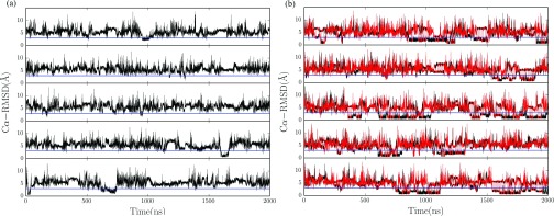
The time series of C_α-RMSD of five independent trajectories using (a) CST method, (b) PCST method, with the red line and black line representing high temperature copy and low temperature copy, respectively. The blue line in each trajectory indicates the 3 Å RMSD. The total simulation time was 2000 ns for each trajectory.

In Figure 3(b), we show the C_α-RMSD of five trajectories using the PCST method. It can be seen that the occurrence of folding events was significantly increased comparing with that of the CST method. Two copies are used in our simulation, one for high temperature and the other for low temperature. For the low temperature copy, the average fraction of time near the native state was 23.7%, with the smallest value 12% and the largest value 42%. For the high temperature copy, the average fraction was 12.8%, with the smallest value 7% and the largest value 20%. The results were achieved by the collaboration of two copies: the low temperature copy is mainly responsible for searching in the folding temperature range, while the high temperature copy is mainly responsible for barrier crossing.

The relationship between RMSD and radius of gyration (R_g) of Cα atoms in the PCST method for both copies is shown in Figure 4. As the peaks of temperature distribution in two copies are 445 K and 316 K, respectively, while the experimental folding temperature is 315 K,^25,32 we can approximately use the RMSD-R_g relationship of two copies to observe the compaction of structure above or around the folding temperature. It is clear that both simulation copies have substantial populations at near native state. In Figure 4(a), the copy samples at high temperature have a significant population in a region around 5 Å RMSD from the native state. In Figure 4(b), for the copy samples around the folding temperature, the near native state region is the only favored region. It is worth mentioning, in high temperature copy simulation, that the R_g of the population peak around 5 Å RMSD is similar to the native state, indicating that this peak corresponds to a state that the hydrophobic collapse has already happened (molten globular state) and that an enormous entropic barrier is present moving from molten globular state to the native state. The barrier between this state and the native state is very eminent. Such results indicate that the generalized ensemble sampling methods are useful in exploring free energy landscape and characterizing the folding transition states, even though the timescale in this kind of simulations is not realistic.

FIG. 4.

Normalized joint distribution of the radius of gyration (R_g) versus RMSD of C_α atoms in (a) high temperature copy and (b) low temperature copy in the PCST method.

The normalized RMSD distributions of two methods are shown in Figures 5(a) and 5(b). Compared to the CST method, the PCST method allows the system to sample near the native state more thoroughly, so the population in the low RMSD range is enhanced. Furthermore, in the distribution of the PCST method, two distinct peaks were observed around 1 Å and 2 Å RMSD, respectively. This seems to suggest that there are two substates near the native state. This phenomenon can also be easily seen in Figure 3(b). We show the amplified parts of trajectory 3 and 5 (Figure 6(a)) along with the molecular structures of the two substates (Figure 6(b)). Between the two substates, the N-terminal helixes of the two structures are almost the same, and differences between the two are mainly caused by the C-terminal polyproline region. Our observation is consistent with the previous computational^33,34 and experimental^34,35 studies about the existence of these two substates.

FIG. 5.

The C_α-RMSD distributions. (a) is for PCST method. The dashed and solid lines denote the distribution in the high temperature copy and low temperature copy, respectively. (b) is for the CST method.

FIG. 6.

(a) Enlargement of parts of traj 3 and traj 5 from Fig. 3(b). The selected time windows are 300–500 ns for traj 3 and 1500–1800 ns for traj 5. The blue line in each trajectory indicates 3 Å RMSD. The RMSD below 3 Å clearly shows two different substates. (b) Molecular structure of two substates. The two structures are aligned with respect to the N-terminal helix (residues 1–10). Two important residues, Pro17 and Pro19, whose sidechains show big difference between two substates, are explicitly drawn. Another residue Ser14, from which large difference of C-alpha trace between the two substates can be seen, is also indicated. The difference between the two substates is mainly in the C-terminal proline-rich loop.

To further characterize the nature of the two substates, we analyzed the C_α-C_α(helix) RMSD distribution for the PCST method (Figure 7), where C_α(helix) represents the C_α atoms in the N-terminal helix formed by the first 10 residues. Results of both copies show that the two substates have almost the same C_α(helix) RMSD, and the difference in the C_α RMSD is caused by the long polyproline in C-terminal region. We have found that there seems to be two distinct types of pathway from the collapsed state (the 5 Å RMSD region mentioned before) to the native state, one type is direct folding to the either substate of the native state (indicated by arrow I and II in Figure 7) and the other type is first folding the N-terminal helix to the native state followed by the folding of flexible polyproline region to the native state (indicated by arrow III in Figure 7). As the two substates were not observed in the CST method, the results of PCST method demonstrate that the existence of the low temperature copy provides more thorough sampling of the free energy landscape near the native state.

FIG. 7.

Normalized joint distribution of the RMSD of C_α with respect to the N-terminal helix versus that with respect to the whole chain, in (a) high temperature copy and (b) low temperature copy using PCST methods. In both cases, three pathways to the native state are indicated as I, II, and III.

IV. CONCLUDING DISCUSSION

In this paper, we present a PCST method which enables parallel copies of simulation to explore the CS collaboratively. A Gaussian distribution in temperature space with different parameters is added on each copy so that it can focus on searching the temperature range around the peak of Gaussian distribution. An exchange protocol of parameters is introduced to eliminate the broken ergodcity issue that might exist in the low temperature copies. PCST inherits the ideas in CST method^12,13 in using continuous tempering, while borrows the spirits in parallel tempering (PT) methods^16,17 in using multiple copies of simulation. The employment of various distributions in different copies overcomes the dilemma between barrier-crossing efficiency and importance sampling in particular temperature range, especially in the low temperature range. As the overlap between temperature distributions is sufficient, the exchange rate between copies can be kept at a relatively high value. At the same time, the exchange rate does not dramatically depend on the system size, which allows one to use much smaller number of copies compared to the conventional PT method. Therefore, it can serve as a good alternative for conventional PT in simulating large systems such as phase transition and dynamics of macromolecules in explicit solvent.

In the simulation of two-dimensional Ising model and Lennard-Jones fluid, we have shown that the desired temperature distribution in each copy can be generated correctly in the long simulation. Not only physical properties can be estimated accurately, the convergence speed of them in the whole temperature range is enhanced as well compared to the single-copy method. Especially for the low temperature copy, the introduction of exchange protocol ensures that it can sample various regions and minima in the CS, which accelerates the convergence of physical properties.

PCST also shows its special effectiveness in protein folding simulation, in which the long residing time in low temperature range is required. In the application of folding trp-cage protein, we observed a significant enhancement of occurrence of the native state compared to the CST method in all the trajectories. In addition, the abundant availability of the native states brings the observation of the existence of two substates in the native region. The molecular structures of two substates are in agreement with the previous computational^33,34 and experimental^34,35 studies. Moreover, three possible folding pathways are observed in the analyzing of C_α-C_α(helix) RMSD relationship, which indicates that various mechanisms might exist in the folding of trp-cage protein. The detection of two substates and multiple possible pathways demonstrates that the PCST method can sample the free energy landscape of protein folding thoroughly.

In PCST method, the number of simulation copy is much smaller than conventional PT, or replica exchange. In protein folding simulations in explicit solvent, for instance, the PCST method typically needs 2–3 copies, while the PT methods commonly use 30–40 copies or more. The centers and widths of the Gaussian distribution in temperature space are empirical parameters to be determined based on the nature of system. For example, in the folding of trp-cage, the low temperature copy distribution was positioned at 316 K which was around the melting temperature of this polypeptide^22,29 so it is set to facilitate enhanced sampling in the compact state of the system. The center of Gaussian for high temperature copy was at 445 K, which was set to facilitate effective barrier crossing. The widths of two Gaussians were adjusted to ensure 30%–40% exchange rate. In folding of even larger systems with higher energy barriers, one may need even wider total temperature range, then one copy could be set at low temperature, one copy at high temperature, and some intermediate copies would also be desirable to bridge the entire temperature range.

REFERENCES

- 1.Frenkel D. and Smit B., Understanding Molecular Simulation: From Algorithms to Applications (Academic Press, 2001). [Google Scholar]
- 2.Mitsutake A., Sugita Y., and Okamoto Y., Biopolymers 60, 96–123 (2001). [DOI] [PubMed] [Google Scholar]
- 3.Berg B. A. and Neuhaus T., Phys. Rev. Lett. 68, 9–12 (1992). 10.1103/PhysRevLett.68.9 [DOI] [PubMed] [Google Scholar]
- 4.Baumann B., Nucl. Phys. B 285, 391–409 (1987). 10.1016/0550-3213(87)90346-4 [DOI] [Google Scholar]
- 5.Wang F. G. and Landau D. P., Phys. Rev. Lett. 86, 2050–2053 (2001); 10.1103/PhysRevLett.86.2050 [DOI] [PubMed] [Google Scholar]; Dayal P.et al. , Phys. Rev. Lett. 92, 097201 (2004). 10.1103/PhysRevLett.92.097201 [DOI] [PubMed] [Google Scholar]
- 6.Yan Q. L., Faller R., and de Pablo J. J., J. Chem. Phys. 116, 8745–8749 (2002); 10.1063/1.1463055 [DOI] [Google Scholar]; Yan Q. L. and de Pablo J. J., Phys. Rev. Lett. 90, 035701 (2003); 10.1103/PhysRevLett.90.035701 [DOI] [PubMed] [Google Scholar]; Shell M. S., Debenedetti P. G., and Panagiotopoulos A. Z., Phys. Rev. E 66, 056703 (2002). 10.1103/PhysRevE.66.056703 [DOI] [PubMed] [Google Scholar]
- 7.Hansmann U. H. E. and Okamoto Y., J. Comput. Chem. 14, 1333–1338 (1993); 10.1002/jcc.540141110 [DOI] [Google Scholar]; Hao M. H. and Scheraga H. A., J. Phys. Chem. 98, 4940–4948 (1994); 10.1021/j100069a028 [DOI] [Google Scholar]; Irback A. and Potthast F., J. Chem. Phys. 103, 10298–10305 (1995). 10.1063/1.469931 [DOI] [Google Scholar]
- 8.Jiang P., Yasar F., and Hansmann U. H. E., J. Chem. Theory Comput. 9, 3816–3825 (2013); 10.1021/ct400312d [DOI] [PMC free article] [PubMed] [Google Scholar]; Zhang C. and Deem M. W., J. Chem. Phys. 138, 034103 (2013). 10.1063/1.4773435 [DOI] [PubMed] [Google Scholar]
- 9.Marinari E. and Parisi G., Europhys. Lett. 19, 451–458 (1992). 10.1209/0295-5075/19/6/002 [DOI] [Google Scholar]
- 10.Hansmann U. H. E. and Okamoto Y., Phys. Rev. E 54, 5863–5865 (1996). 10.1103/PhysRevE.54.5863 [DOI] [PubMed] [Google Scholar]
- 11.Zhang C. and Ma J., Phys. Rev. E 76, 036708 (2007). 10.1103/PhysRevE.76.036708 [DOI] [PMC free article] [PubMed] [Google Scholar]
- 12.Zhang C. and Ma J., J. Chem. Phys. 130, 194112 (2009). 10.1063/1.3139192 [DOI] [PMC free article] [PubMed] [Google Scholar]
- 13.Zhang C. and Ma J., J. Chem. Phys. 132, 244101 (2010). 10.1063/1.3435332 [DOI] [PMC free article] [PubMed] [Google Scholar]
- 14.Zhang C. and Ma J., J. Chem. Phys. 129, 134112 (2008). 10.1063/1.2988339 [DOI] [PMC free article] [PubMed] [Google Scholar]
- 15.Liu Y. X.et al. , J. Phys. Chem. Lett. 3, 1117–1123 (2012); 10.1021/jz300017c [DOI] [PMC free article] [PubMed] [Google Scholar]; Zhang C. and Ma J., Proc. Natl. Acad. Sci. U.S.A. 109, 8139–8144 (2012). 10.1073/pnas.1112143109 [DOI] [PMC free article] [PubMed] [Google Scholar]
- 16.Gilmanshin R.et al. , Proc. Natl. Acad. Sci. U.S.A. 94, 3709–3713 (1997); 10.1073/pnas.94.8.3709 [DOI] [PMC free article] [PubMed] [Google Scholar]; Eaton W. A.et al. , Annu. Rev. Biophys. Biomol. Struct. 29, 327–359 (2000). 10.1146/annurev.biophys.29.1.327 [DOI] [PMC free article] [PubMed] [Google Scholar]
- 17.Swendsen R. H. and Wang J. S., Phys. Rev. Lett. 58, 86–88 (1987); 10.1103/PhysRevLett.58.86 [DOI] [PubMed] [Google Scholar]; Wolff U., Phys. Rev. Lett. 62, 361–364 (1989). 10.1103/PhysRevLett.62.361 [DOI] [PubMed] [Google Scholar]
- 18.Swendsen R. H. and Wang J. S., Phys. Rev. Lett. 57, 2607–2609 (1986). 10.1103/PhysRevLett.57.2607 [DOI] [PubMed] [Google Scholar]
- 19.Falcioni M. and Deem M. W., J. Chem. Phys. 110, 1754–1766 (1999); 10.1063/1.477812 [DOI] [Google Scholar]; Sugita Y. and Okamoto Y., Chem. Phys. Lett. 314, 141–151 (1999); 10.1016/S0009-2614(99)01123-9 [DOI] [Google Scholar]; Earl D. J. and Deem M. W., Phys. Chem. Chem. Phys. 7, 3910–3916 (2005). 10.1039/b509983h [DOI] [PubMed] [Google Scholar]
- 20.Neal R. M., Stat. Comput. 6, 353–366 (1996). 10.1007/BF00143556 [DOI] [Google Scholar]
- 21.Rhee Y. M. and Pande V. S., Biophys. J. 84, 775–786 (2003); 10.1016/S0006-3495(03)74897-8 [DOI] [PMC free article] [PubMed] [Google Scholar]; Kim J., Keyes T., and Straub J. E., J. Chem. Phys. 132, 224107 (2010); 10.1063/1.3432176 [DOI] [PMC free article] [PubMed] [Google Scholar]; Kim J., Straub J. E., and Keyes T., J. Phys. Chem. B 116, 8646–8653 (2012). 10.1021/jp300366j [DOI] [PMC free article] [PubMed] [Google Scholar]
- 22.Tolman R. C., The Principles of Statistical Mechanics (Oxford at the Clarendon Press, 1938). [Google Scholar]
- 23.Berendsen H. J. C., Vanderspoel D., and Vandrunen R., Comput. Phys. Commun. 91, 43–56 (1995); 10.1016/0010-4655(95)00042-E [DOI] [Google Scholar]; Lindahl E., Hess B., and van der Spoel D., J. Mol. Model. 7, 306–317 (2001); 10.1007/s008940100045 [DOI] [Google Scholar]; Van der Spoel D.et al. , J. Comput. Chem. 26, 1701–1718 (2005); 10.1002/jcc.20291 [DOI] [PubMed] [Google Scholar]; Hess B.et al. , J. Chem. Theory Comput. 4, 435–447 (2008). 10.1021/ct700301q [DOI] [PubMed] [Google Scholar]
- 24.Rowley L. A., Nicholson D., and Parsonage N. G., J. Comput. Phys. 17, 401–414 (1975). 10.1016/0021-9991(75)90042-X [DOI] [Google Scholar]
- 25.Neidigh J. W., Fesinmeyer R. M., and Andersen N. H., Nat. Struct. Biol. 9, 425–430 (2002). 10.1038/nsb798 [DOI] [PubMed] [Google Scholar]
- 26.Wang J. M., Cieplak P., and Kollman P. A., J. Comput. Chem. 21, 1049–1074 (2000); [DOI] [Google Scholar]; Hornak V.et al. , Proteins 65, 712–725 (2006). 10.1002/prot.21123 [DOI] [PMC free article] [PubMed] [Google Scholar]
- 27.Jorgensen W. L.et al. , J. Chem. Phys. 79, 926–935 (1983). 10.1063/1.445869 [DOI] [Google Scholar]
- 28.Essmann U.et al. , J. Chem. Phys. 103, 8577–8593 (1995). 10.1063/1.470117 [DOI] [Google Scholar]
- 29.Hess B., J. Chem. Theory Comput. 4, 116–122 (2008). 10.1021/ct700200b [DOI] [PubMed] [Google Scholar]
- 30.Miyamoto S. and Kollman P. A., J. Comput. Chem. 13, 952–962 (1992). 10.1002/jcc.540130805 [DOI] [Google Scholar]
- 31.Bussi G., Donadio D., and Parrinello M., J. Chem. Phys. 126, 014101 (2007). 10.1063/1.2408420 [DOI] [PubMed] [Google Scholar]
- 32.Qiu L. L.et al. , J. Am. Chem. Soc. 124, 12952–12953 (2002). 10.1021/ja0279141 [DOI] [PubMed] [Google Scholar]
- 33.Marino K. A. and Bolhuis P. G., J. Phys. Chem. B 116, 11872–11880 (2012); 10.1021/jp306727r [DOI] [PubMed] [Google Scholar]; Shao Q., Shi J. Y., and Zhu W. L., J. Chem. Phys. 137, 125103 (2012). 10.1063/1.4754656 [DOI] [PubMed] [Google Scholar]
- 34.Meuzelaar H.et al. , J. Phys. Chem. B 117, 11490–11501 (2013). 10.1021/jp404714c [DOI] [PubMed] [Google Scholar]
- 35.Rovo P.et al. , J. Pept. Sci. 17, 610–619 (2011). 10.1002/psc.1377 [DOI] [PubMed] [Google Scholar]
- 36.Hunter J. D., Comput. Sci. Eng. 9, 90–95 (2007). 10.1109/MCSE.2007.55 [DOI] [Google Scholar]
- 37. Schrodinger, LLC, 2010.