Smoothing fields of weighted collections with applications to diffusion MRI processing

Abstract

Using modern diffusion weighted magnetic resonance imaging protocols, the orientations of multiple neuronal fiber tracts within each voxel can be estimated. Further analysis of these populations, including application of fiber tracking and tract segmentation methods, is often hindered by lack of spatial smoothness of the estimated orientations. For example, a single noisy voxel can cause a fiber tracking method to switch tracts in a simple crossing tract geometry. In this work, a generalized spatial smoothing framework that handles multiple orientations as well as their fractional contributions within each voxel is proposed. The approach estimates an optimal fuzzy correspondence of orientations and fractional contributions between voxels and smooths only between these correspondences. Avoiding a requirement to obtain exact correspondences of orientations reduces smoothing anomalies due to propagation of erroneous correspondences around noisy voxels. Phantom experiments are used to demonstrate both visual and quantitative improvements in postprocessing steps. Improvement over smoothing in the measurement domain is also demonstrated using both phantoms and in vivo human data.

1. INTRODUCTION

Over the past dozen years, many methods to reconstruct neuronal fiber tracts in human white matter from diffusion MRI data have been reported.¹ Early methods used only a single direction at each voxel,² but with newer diffusion MRI acquisition protocols the opportunity to exploit multiple directions and their fractional contributions—generically referred to as multi-tensor models^{3, 4}—within each voxel have been developed.^{5, 6} The performance of these methods depends strongly on accurate orientation information at each voxel, and it is common to carry out repeated scans in order to provide such data. But acquisition of repeated scans comes at the cost of increasing scan time, and the effort may still not be sufficient to remove noise sufficiently to permit optimal tractography. Thus, postprocessing data for noise removal has been explored, and is the subject of the work reported here.

One way to address noise in diffusion MRI data is to smooth the raw data. For example, Jeurissen et al.⁷ used the adaptive anisotropic noise filtering method of Sijbers et al.⁸ in their MICCAI fiber cup challenge result.¹ As well, Kuurstra et al.⁹ used a nonlocal means approach, and McGraw et al.¹⁰ used an image restoration approach specified by a variational formulation. Another point at which to carry out smoothing is after tensor reconstruction. For example, Tabelow et al.¹¹ and Chen et al.¹² developed different approaches to smooth tensor fields. However, neither method generalizes to multi-tensor models or other representations specifying multiple orientations at each voxel. Although the smoothing of raw data can certainly be carried out in multi-tensor and multi-orientation models (since it applies before the analysis phase), the smoothing of multi-tensor or multi-orientation fields remains an open problem.

In this work we present a method to spatially smooth an orientation field that has been estimated from the raw (or smoothed) diffusion MRI data. The method considers both multiple orientations and their fractional contributions—i.e., their memberships—within each voxel. In order to smooth between voxels, a correspondence of orientations between each pair of voxels is first solved. A unique aspect of the present work is that a fuzzy correspondence that involves both the collection of orientations and their fractional contributions is produced by solving an optimization criterion. In this way, smoothing is carried out between populations that are likely to be associated with each other while erroneous orientation associations are avoided. Benefits of this approach are demonstrated on simulated phantom and in vivo data.

2. SMOOTHNESS ENERGY FUNCTION

The observed data are orientations ω_i and associated fractional contributions f_i, i = 1, …, N at a collection of 3D spatial locations Ω. The orientations are unit vectors belonging to the sphere and ω and −ω are assumed to be equivalent. At voxel A ∈ Ω, the fractional contributions $f_i^A$ sum to unity. In this work, we assume the fractional contributions to be correct but the orientations are subject to error, and our goal is to modify the orientations in order to reflect smooth spatial transitions of the orientations. The main objective at this stage is to find correspondences between voxels so that smoothing can take place across “like” populations.

Consider the voxel A and another voxel B that is in the neighborhood of A. Let the distance between two orientations ${\mathit{\omega }}_i^A$ and ${\mathit{\omega }}_j^B$, one from voxel A and the other from voxel B, be given by $d({\mathit{\omega }}_i^A,{\mathit{\omega }}_j^B)$. Here, we simply let this distance be the arclength along the great circle on the unit sphere between the two unit vectors. We let the two fiber populations defined by these two orientations to be associated with each other by an unknown weight $w_{ij}^{AB}$. The roughness of the entire population can therefore be defined by an energy function as follows

$$E=\sum _{A\in \mathrm{\Omega }}\sum _{B\in {\mathcal{N}}_A}\sum _{i=1}^N\sum _{j=1}^N{w}_{ij}^{AB}{d}^2({\mathit{\omega }}_i^A,{\mathit{\omega }}_j^B).$$ (1)

The entire population can be made smoother by reducing E, and this can happen either by selecting the weights w to minimize the impact of large distances between the orientations of adjacent voxels or by changing the orientations themselves. The first step is equivalent to finding associations between the orientations of adjacent voxels and the second step is equivalent to smoothing the orientations. The problem can be better understood by considering the graph shown in Figure 1, which illustrates the problem with three orientations at each voxel.

Figure 1.

Demonstration of the weights in equation (1), showing that the equation is composed of relationships between all neighboring voxels.

This framework is further developed by constraining the values of w to reflect the fractional contributions, ${\sum }_j{w}_{ij}^{AB}=f_i^A$ and ${\sum }_i{w}_{ij}^{AB}=f_j^B$. Under these constraints, minimizing equation (1) with respect w for fixed ω can be interpreted as finding the smoothest association between voxels. By treating $w_{ij}^{AB}$ as elements of the matrix W^AB, we can write this constraint as follows

$${\mathbf{f}}^B=W^{AB}\mathbf{1},{\mathbf{f}}^A={\left(W^{AB}\right)}^{\top }\mathbf{1},w_{ij}^{AB}\ge 0,$$ (2)

where the i-th element of f^B is $f_i^B$. Revisiting the graph interpretation, this can be interpreted as the sum of all edges that connect to a vertex (between two voxels) is the fractional contribution of that vertex. With this constraint the energy function becomes

$$E=\underset{\mathbf{w}}{min}\sum _{A\in \mathrm{\Omega }}\sum _{B\in {\mathcal{N}}_A}\sum _{i=1}^N\sum _{j=1}^N{w}_{ij}^{AB}{d}^2({\mathit{\omega }}_i^A,{\mathit{\omega }}_j^B)\mathrm{s}.\mathrm{t}.{\mathbf{f}}^B=W^{AB}\mathbf{1},{\mathbf{f}}^A={(W^{AB})}^{\top }\mathbf{1},w_{ij}^{AB}\ge 0,$$ (3)

where w is the set of all $w_{ij}^{AB}$. For the smoothing step, this energy function is decreased by changing ω. For a given ω, the minimum energy configuration for w is found by solving a linear programming problem between each pair of neighboring voxels and results in an undirected fuzzy match—i.e., not a one-to-one match—between orientations in voxels A and B. That is

$$W^{AB}=\underset{w_{ij}^{AB}\ge 0}{argmin}\sum _i\sum _j{w}_{ij}^{AB}{d}_{ij}\mathrm{s}.\mathrm{t}.{\mathbf{f}}^B=W^{AB}\mathbf{1},{\mathbf{f}}^A={(W^{AB})}^{\top }\mathbf{1}$$ (4)

$$=\underset{w_{ij}^{AB}\ge 0}{argmin}\langle \left[\begin{array}{c}{w}_{11}^{AB}\\ w_{12}^{AB}\\ ⋮\\ w_{21}^{AB}\\ ⋮\\ w_{NN}^{AB}\end{array}\right],\left[\begin{array}{c}{d}_{11}\\ d_{12}\\ ⋮\\ d_{21}\\ ⋮\\ d_{NN}\end{array}\right]\rangle \mathrm{s}.\mathrm{t}.\left[\begin{array}{c}{f}_1^B\\ ⋮\\ f_N^B\end{array}\right]=F\left[\begin{array}{c}{w}_{11}^{AB}\\ w_{12}^{AB}\\ ⋮\\ w_{21}^{AB}\\ ⋮\\ w_{NN}^{AB}\end{array}\right]\text{and}\left[\begin{array}{c}{f}_1^A\\ ⋮\\ f_N^A\end{array}\right]=S\left[\begin{array}{c}{w}_{11}^{AB}\\ w_{12}^{AB}\\ ⋮\\ w_{21}^{AB}\\ ⋮\\ w_{NN}^{AB}\end{array}\right],$$ (5)

where $d_{ij}=d^2({\mathit{\omega }}_i^A,{\mathit{\omega }}_j^B)$ and

$$S=\left[\begin{array}{ccccccccccccc}1& 1& \dots & 1& & & & & & & & & \\ & & & & 1& 1& \dots & 1& & & & & \\ & & & & & & & & \ddots & & & & \\ & & & & & & & & & 1& 1& \dots & 1\end{array}\right]$$ (6)

$$F=\left[\begin{array}{ccccccccccccc}1& & & & 1& & & & & 1& & & \\ & 1& & & & 1& & & \dots & & 1& & \\ & & \ddots & & & & \ddots & & & & & \ddots & \\ & & & 1& & & & 1& & & & & 1\end{array}\right].$$ (7)

3. SMOOTHING

For the smoothing step, iterations of gradient descent optimization are applied on ω for fixed w. The energy function is rewritten as follows

$$E=\sum _{A\in \mathrm{\Omega }}\sum _{i=1}^N\left(\sum _{B\in {\mathcal{N}}_A}\sum _{j=1}^N{w}_{ij}^{AB}{d}^2({\mathit{\omega }}_i^A,{\mathit{\omega }}_j^B)\right).$$ (8)

That is, for every orientation in every voxel, the weighted distance to neighbouring orientations is minimized. For efficient gradient descent, the orientation minimizing the weighted distance to the neighboring orientation is calculated and it is assumed that the initial orientation is relatively close to this minimum. (This is the same as assuming that the data is sufficiently smooth). Utilizing these assumptions, the step along the gradient is approximated by stepping towards the minimum. This gradient descent step can be shown to equal updating every orientation with a weighted average of its associated orientations in all neighboring voxels. Thus, smoothing is done in proper proportion to the currently estimated population associations and is stepwise, leading to increasing smoothing with repeated iterations of the two alternating steps. In Euclidean space, ${\mathbf{x}}_i^A\in {ℝ}^n$, the update equation would be as follows

$${\mathbf{x}}_i^A\leftarrow \frac{1}{2}{\mathbf{x}}_i^A+\frac{1}{2}\frac{{\sum }_{B\in N_A}{\sum }_j{w}_{ij}^{AB}{\mathbf{x}}_j^B}{{\sum }_{B\in {\mathcal{N}}_A}{\sum }_j{w}_{ij}^{AB}}$$ (9)

where ${\sum }_{B\in {\mathcal{N}}_A}{\sum }_j{w}_{ij}^{AB}=\mid {\mathcal{N}}_A\mid f_i^A$, and | | is the number of neighbors of A. By assuming a 6-connected neighborhood, and using the fact that $w_{ij}^{AB}=w_{ji}^{BA}$ we can rewrite Equation (9) in one dimension as follows

$${\mathbf{x}}_i^B\leftarrow \frac{{\sum }_j{w}_{ji}^{AB}{\mathbf{x}}_j^A+2f_i^B{\mathbf{x}}_i^B+{\sum }_j{w}_{ij}^{BC}{\mathbf{x}}_j^C}{4f_i^B},$$ (10)

where A is the previous voxel, B is the current voxel, and C is the next voxel. This allows for calculating half as many coefficients. However, this weighted average must be along the geodesic, and Section 4 presents a fast algorithm for approximating this calculation.

It is interesting to note the similarity with moving average filtering. The notable difference, is that since there are collections of orientations, standard filtering methods are inapplicable. The described method applies filtering by finding the orientations in the neighboring voxels that correspond to a given orientation—along with a belief in that correspondence. Using those memberships a moving average filter is applied along the geodesic.

4. IMPLEMENTATION

There are certain problems with implementing the algorithm above that need addressing. First, to improve robustness to outliers and imperfect matches, it is useful to zero weights that correspond to orientations more than 45° apart. Second, a fast, approximate algorithm for averaging orientations is described in Algorithm 1. This algorithm aligns the orientations such that they point in the same direction as the estimated orientation e, finds the average in Euclidean space, and projects the result to the unit sphere. This is an adequate assumption granted the orientations are in a 90° cone.

Algorithm 1.

Simple Weighted Average of Orientations

Require: ω (The Orientations), γ (The Weights), e (The Original Estimate).

si = sign(〈xi, e〉)

ωi = siωi

y = Σi γiωi

return $\frac{\mathbf{y}}{{\Vert \mathbf{y}\Vert }_2}$

An example implementation for smoothing along a single spatial direction is demonstrated in Algorithm 2. MATLAB implementation is available on the authors’ website (http://iacl.ece.jhu.edu/gunnar) and a Java implementation is included in the Java Image Science Toolkit (http://www.nitrc.org/projects/jist/).

Algorithm 2.

Smoothing voxel B along one dimension

Require: ωA, ωB, ωC (Orientations), WAB, WBC (Weights), cutoff (Cutoff Threshold)

for all ${\mathit{\omega }}_i^B\in {\mathit{\omega }}^B$ do

${\alpha }_j=\frac{w_{ji}^{AB}}{{\sum }_j{w}_{ji}^{AB}}$

${\beta }_j=\frac{w_{ji}^{BC}}{{\sum }_j{w}_{ij}^{BC}}$

${\alpha }_j=0\text{if}\mid \langle {\mathit{\omega }}_j^A,{\mathit{\omega }}_i^B\rangle \mid <\text{cutoff}$

${\beta }_j=0\text{if}\mid \langle {\mathit{\omega }}_j^C,{\mathit{\omega }}_i^B\rangle \mid <\text{cutoff}$

γ = [α1, …, αN, 2, β1, …, βN]⊤

$\mathit{\xi }={\left[{\mathit{\omega }}^A,{\mathit{\omega }}_i^B,{\mathit{\omega }}^C\right]}^{\top }$

${{}^{\text{new}}\mathit{\omega }}_i^B=\text{weightedAverage}(\mathit{\xi },\mathit{\gamma },{\mathit{\omega }}_i^B)$

end for

return newωB

5. RESULTS

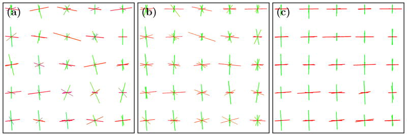
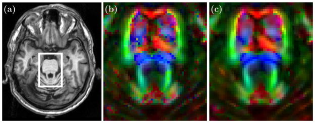
To demonstrate the performance of this smoothing algorithm we first applied it to a multi-tensor crossing fiber computational phantom having crossing fibers at right angles in the plane. The reconstruction algorithm CFARI⁴ was used to recover the directions and fractional contributions from noisy observations. Figure 2 shows the CFARI directions (a) and the smoothed result (b) after five iterations. The smoothed result is then further processed to remove correspondences whose separation angle is greater than 45° (c). Figure 3 compares smoothing on a different crossing phantom with smoothing in the measurement domain by a Gaussian filter of similar size. All filtering was done in the plane. It is observed that two populations tend to emerge, and they are at the correct angles. Figure 4 shows a result of smoothing in vivo human data, where CFARI⁴ was used to estimate the directions and their fractional contributions from a Jones-30, b = 700 s/mm² acquisition. The orientations are visualized in both before and after images by finding the weighted average direction at each voxel and using a standard DTI color map: red (left/right), green (anterior/posterior), and blue (inferior/superior). (These are multiplied by FA, computed from the usual tensor estimate.)

Figure 2.

The crossing phantom (a) before, (b) after smoothing, and (c) with processing. The green color represents up/down and red left/right. The length of a direction represents its fractional contribution.

Figure 3.

The varying crossing phantom (a) without any smoothing, (b) after Gaussian smoothing with σ = 4 voxels, and (c) after 10 iterations of the proposed method.

Figure 4.

(a) The corticospinal tract and the transverse pontine fibers (b) before and (c) after smoothing.

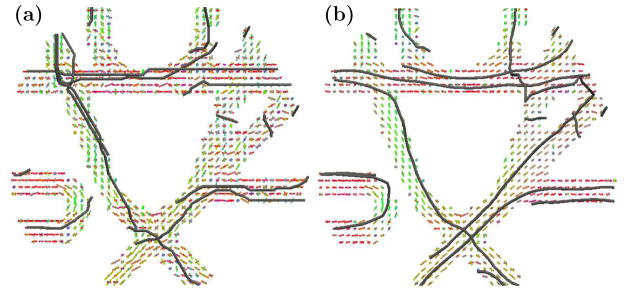
Finally, Figure 5 and Figure 6 show tractography results. In Figure 5 we used a decimated version of the publicly available MICCAI Fiber Cup phantom in order to demonstrate performance under a low-quality sampling scheme (30 scanning directions). Simple tractography was carried out by following the direction at each voxel most similar to the previous direction. Fiber tracking was initiated from a small collection of seeds given in the MICCAI Fiber Cup Challenge.¹ It is clear that the proposed smoothing method can enhance the quality of fiber tract reconstruction and preserve crossing regions. Figure 6 demonstrates tractography with smoothing on a human subject (Jones-30, b = 700 s/mm² acquisition). CFARI⁴ was used to estimate directions and fractional contributions, and INFACT⁴ was used for fiber tracking. We see that even when looking only at fibers that connect two specific regions of interest, there is qualitative improvement by applying the smoothing method prior to performing tractography.

Figure 5.

Fiber tracking on the decimated Fiber Cup Phantom (a) before and (b) after 10 iterations of smoothing.

Figure 6.

Coronal view of tractography of the internal capsule (a) before and (b) after smoothing, superimposed on a DTI color map. The crossing with the corpus callosum is preserved (c).

6. CONCLUSIONS

We presented an energy minimization framework for smoothing orientations derived from diffusion weighted imaging and multi-tensor estimation. Its performance was demonstrated on computational phantoms and human in vivo data. The main result of this work is that presented with corrupted measurements of multiple superimposed populations of orientations, if the populations themselves are sufficiently smooth, the method correctly reconstructs the correspondences, and the following smoothing enhances the populations without blending them. The method demonstrated advantages over smoothing in the measurement domain, and since it exploits different principles, it may be combined with existing methods for smoothing in the measurement domain. We hope that this work may raise interest in utilizing correspondences for approaching problems in multi-tensor tractography and in the analysis of crossing regions in human white matter.

References

- 1.Fillard P, Descoteaux M, Goh A, Gouttard S, Jeurissen B, Malcolm J, Ramirez-Manzanares A, Reisert M, Sakaie K, Tensaouti F, et al. Quantitative evaluation of 10 tractography algorithms on a realistic diffusion mr phantom. Neuroimage. 2011;56(1):220–234. doi: 10.1016/j.neuroimage.2011.01.032. [DOI] [PubMed] [Google Scholar]
- 2.Mori S, Crain BJ, Chacko V, Van Zijl P. Three-dimensional tracking of axonal projections in the brain by magnetic resonance imaging. Annals of neurology. 1999;45(2):265–269. doi: 10.1002/1531-8249(199902)45:2<265::aid-ana21>3.0.co;2-3. [DOI] [PubMed] [Google Scholar]
- 3.Peled S, Friman O, Jolesz F, Westin CF. Geometrically constrained two-tensor model for crossing tracts in dwi. Magnetic resonance imaging. 2006;24(9):1263–1270. doi: 10.1016/j.mri.2006.07.009. [DOI] [PMC free article] [PubMed] [Google Scholar]
- 4.Landman BA, Bogovic JA, Wan H, ElShahaby FEZ, Bazin PL, Prince JL. Resolution of crossing fibers with constrained compressed sensing using diffusion tensor mri. Neuro Image. 2012;59(3):2175–2186. doi: 10.1016/j.neuroimage.2011.10.011. [DOI] [PMC free article] [PubMed] [Google Scholar]
- 5.Kreher B, Schneider J, Mader I, Martin E, Hennig J, Il’yasov K. Multitensor approach for analysis and tracking of complex fiber configurations. Magnetic resonance in medicine. 2005;54(5):1216–1225. doi: 10.1002/mrm.20670. [DOI] [PubMed] [Google Scholar]
- 6.Bergmann O, Kindlmann G, Peled S, Westin C-F. Two-tensor fiber tractography. Biomedical Imaging: From Nano to Macro, 2007. ISBI 2007. 4th IEEE International Symposium on; IEEE; 2007. pp. 796–799. [Google Scholar]
- 7.Jeurissen B, Leemans A, Tournier J-D, Sijbers J. Fiber tracking on the fiber cup phantom using constrained spherical deconvolution. Medical Image Computing and Computer-Assisted Intervention (MICCAI) Workshop on Diffusion Modelling and the Fiber Cup (DMFC’09); 2009. pp. 232–235. [Google Scholar]
- 8.Sijbers J, den Dekker AJ, Van der Linden A, Verhoye M, Van Dyck D. Adaptive anisotropic noise filtering for magnitude mr data. Magnetic resonance imaging. 1999;17(10):1533–1539. doi: 10.1016/s0730-725x(99)00088-0. [DOI] [PubMed] [Google Scholar]
- 9.Kuurstra A, Dolui S, Michailovich O. SPIE Medical Imaging. International Society for Optics and Photonics; 2012. Hardi denoising using nonlocal means on s2; pp. 83140I–83140I. [Google Scholar]
- 10.McGraw T, Vemuri B, Özarslan E, Chen Y, Mareci T. Variational denoising of diffusion weighted mri. Inverse Problems and Imaging. 2009;35(4):625. doi: 10.3934/ipi.2009.3.625. [DOI] [PMC free article] [PubMed] [Google Scholar]
- 11.Tabelow K, Polzehl J, Spokoiny V, Voss HU. Diffusion tensor imaging: Structural adaptive smoothing. Neuro Image. 2008;39(4):1763–1773. doi: 10.1016/j.neuroimage.2007.10.024. [DOI] [PubMed] [Google Scholar]
- 12.Chen B, Hsu EW. Noise removal in magnetic resonance diffusion tensor imaging. Magnetic Resonance in Medicine. 2005;54(2):393–401. doi: 10.1002/mrm.20582. [DOI] [PubMed] [Google Scholar]