

Abstract
Background
This represents the first graph theory based brain network analysis study in bipolar disorder, a chronic and disabling psychiatric disorder characterized by severe mood swings. Many imaging studies have investigated white matter in bipolar disorder with results suggesting abnormal white matter structural integrity, particularly in the fronto-limbic and callosal systems. However, many inconsistencies remain in the literature, and no study to-date has conducted brain network analyses using a graph-theoretic approach.
Methods
We acquired 64-direction diffusion-weighted MRI on 25 euthymic bipolar I disorder subjects and 24 gender and age equivalent healthy subjects. White matter integrity measures including fractional anisotropy and mean diffusivity were compared in the whole brain. Additionally, structural connectivity matrices based on whole brain deterministic tractography were constructed followed by the computation of both global and local brain network measures. We also designed novel metrics to further probe inter-hemispheric integration.
Results
Network analyses revealed that the bipolar brain networks exhibited significantly longer characteristic path length, lower clustering coefficient, and lower global efficiency relative to those of controls. Further analyses revealed impaired inter-hemispheric but relatively preserved intra-hemispheric integration. These findings were supported by whole brain white matter analyses that revealed significantly lower integrity in the corpus callosum in bipolar subjects. There were also abnormalities in nodal network measures in structures within the limbic system, especially the left hippocampus, the left lateral orbito-frontal cortex, and the bilateral isthmus cingulate.
Conclusions
These results suggest abnormalities in structural network organization in bipolar disorder, particularly in inter-hemispheric integration and within the limbic system.
Keywords: bipolar disorder, DTI, brain network analysis, brain imaging, hemispheric integration, corpus callosum, limbic system
1. Introduction
Bipolar disorder is associated with anatomical and functional abnormalities in brain regions that mediate emotion regulation (1). Fluctuations of mood and emotion that are hallmarks of the disorder suggest dysfunctions of brain networks that maintain emotional homeostasis. There is increasing evidence suggesting that the mechanism underlying such dysfunctions may include disruptions in white matter integrity. Specifically, several studies have reported a reduction of oligodendrocytes and decreased myelin-related gene expression in bipolar disorder (1-3).
Using diffusion tensor imaging (DTI), widespread lobar microstructural abnormalities have been reported in bipolar disorder in the prefrontal, parietal, temporal, and occipital lobes (4, 5) as well as within the anterior-limbic network (6). Some of the most studied neural circuits in bipolar imaging to-date have focused on the white matter tracts that connect the prefrontal cortex and the limbic system, although other association and projection fiber tracts including internal capsule and superior longitudinal fasciculus have also been implicated (7-9).
Most studies in bipolar disorder have demonstrated some form of impaired white matter integrity; however, there have been some inconsistent results reported in the literature (10-14). For example, reduced fractional anisotropy (FA) suggesting defects in frontal lobe white matter integrity has been reported in one DTI study (11). In contrast, several studies have shown increased FA or higher numbers of reconstructed fibers in certain white matter tracts (1, 15-17). In (4), the authors also reported higher apparent diffusion coefficient (a general measure of the magnitude of local water diffusivity) in bilateral OFC in bipolar patients with no differences in FA. One region that has been extensively studied in bipolar imaging is the corpus callosum. Despite higher FA values in the midline genu reported in (14), most studies to date have demonstrated impaired integrity of the corpus callosum in bipolar disorder (12, 13, 18-20). These findings thus suggest inter-hemispheric communication abnormalities.
In this study, we employed two complementary neuro-imaging techniques to study bipolar disorder. First, we conducted whole brain white matter analyses using DTI measures (FA and MD) to investigate white matter integrity. Additionally, we used graph theory and conducted state-of-the-art brain network analyses. The results from whole brain white matter analyses informed our a priori regions for brain network analyses. As a novel high-level neuroimaging technique, network analyses probe the organizational properties of the human brain as a complex system, by mathematically representing it as a “graph”, which contains the nodes (gray matter) and the edges (white matter) connecting the nodes. Graph metrics that characterize system properties can then be constructed; these metrics have most recently been shown to give additional insight into the human brain's network properties (21-24).
Here, we proposed and tested several a priori hypotheses. First, as converging lines of evidence implicate oligodendrocyte dysfunction in bipolar disorder, we hypothesized that diffusion weighted imaging may reveal signs of abnormal myelination. Thus, subjects with bipolar disorder would exhibit white matter integrity changes (lower FA and/or higher MD) in our whole brain white matter analyses. Based on previous findings implicating fronto-limbic circuitry, for brain network analyses we specifically hypothesized that the following gray matter structures may exhibit node-level abnormalities in bipolar subjects relative to controls: the orbito-frontal cortex, the cingulate, and limbic structures in the temporal lobe (amygdala, parahippocampal gyrus, hippocampus, and entorhinal cortex). Lastly, we also hypothesized abnormalities in the corpus callosum due to its role in inter-hemispheric communication.
2. Materials and Methods
Subject recruitment and informed consent
The sample consisted of 25 participants with bipolar I disorder (14 male and 11 female; age: 41.6 +/- 12.7) and 24 healthy controls (13 male and 11 female; age: 41.6+/- 10.6). All bipolar subjects received comprehensive psychiatric evaluations using the structured clinical interview for DSM disorders (SCID; http://www.scid4.org/) and met the DSM IV criteria for bipolar I disorder. At the time of image acquisition, all subjects were in a euthymic state, operationally defined as a score of less than 7 on both the Young Mania Rating Scale (YMRS)(25) and the Hamilton Rating Scale for Depression (HAM-D) (26) as well as an absence of any mood episodes within 30 days of the scan.
At the time of the MRI scan, 7 participants were on valproic acid, 1 on carbamazepine, 3 on lamotrigine, 14 on antipsychotic medications, 8 on SSRI antidepressant medications, 5 on other antidepressant medications, and 3 on benzodiazepine (none of the study participants was on lithium; two participants were not on any psychotropic medications either at SCID or the time of the MRI scan).
Image acquisition
Diffusion weighted MRI data were acquired on a Siemens 3T Trio scanner. Sixty contiguous axial brain slices were collected using the following parameters: 64 diffusion-weighted (b=1000s/mm2) and 1 non-diffusion weighted scan; field of view (FOV) 190mm by 190mm; voxel size 2×2×2mm; TR=8400ms; TE=93ms. In addition, high-resolution structural images were acquired using T1-weighted magnetization-prepared rapid-acquisition gradient echo (MPRAGE; FOV 250mm by 250 mm; voxel size: 1×1×1mm; TR=1900ms, TE=2.26ms, flip angle=9°).
Image Preprocessing
Figure 1 illustrates the pipeline used for image preprocessing. Briefly, for each subject, whole brain white matter was segmented into 50 regions (Table1) based on the ICBM young adult DTI-81 atlas (http://www.loni.ucla.edu/ICBM/). To this end, we first non-linearly registered atlas FA to individual subject's FA using FNIRT implemented in FSL (http://fsl.fmrib.ox.ac.uk/fsl) to obtain a transformation matrix, which was applied to all atlas white matter ROIs to map them onto the subject's individual space, yielding a total of 50 white matter regions. For brain network analyses, we conducted cortical/subcortical gray matter segmentation in individual subjects' MPRAGE space to yield 87 gray matter regions (68 cortical and 19 subcortical) using Freesurfer (http://surfer.nmr.mgh.harvard.edu/).
Figure 1.
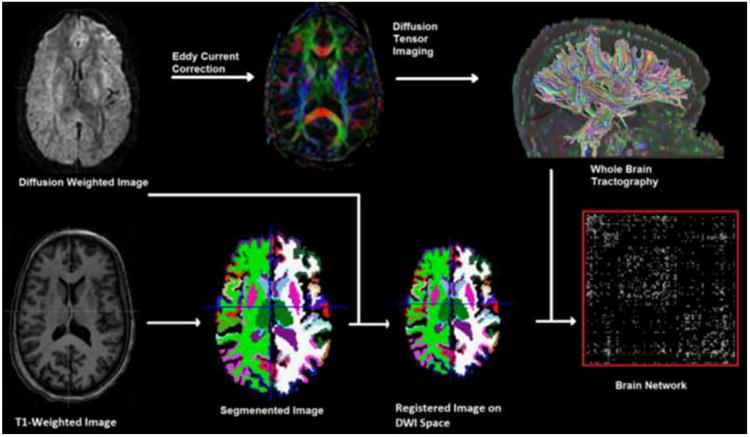
This figure illustrates the pipeline used in this study to construct: DTI white matter integrity measures (top middle panel), whole brain tractography (top right panel), gray matter segmentation (lower middle panels), and the brain network connectivity matrix (lower right panel).
Table 1.
Whole brain white matter parcellated into 50 white matter regions based on the ICBM young adult DTI-81 atlas.
| MCP | Middle cerebellar peduncle | BCC | Body of corpus callosum |
|---|---|---|---|
| PCT | Pontine crossing tract | SCC | Splenium of corpus callosum |
| ICP* | Inferior cerebellar peduncle | GCC | Genu of corpus callosum |
| SCP* | Superior cerebellar peduncle | ACR* | Anterior corona radiata |
| CST* | Corticospinal tract | ML* | Medial lemniscus |
| PCR* | Posterior corona radiata | PTR* | Posterior thalamic radiation |
| SS* | Sagittal stratum | FX | Fornix |
| UNC* | Uncinate fasciculus | TAP* | Tapetum |
| CP* | Cerebral peduncle | EC* | External capsule |
| ALIC* | Anterior limb of internal capsule | RLIC* | Retrolenticular part of internal capsule |
| PLIC* | Posterior limb of internal capsule | FX/ST* | Fornix / Stria terminalis |
| CGH* | Cingulum (hippocampus part) | SLF* | Superior longitudinal fasciculus |
| IFO* | Inferior fronto-occipital fasciculus | SFO* | Superior fronto-occipital fasciculus |
| SCR* | Superior corona radiata | CGC* | Cingulum (cingulate gyrus part) |
indicates tracts that are present in both left and right hemispheres
To generate DTI measures, all images were first corrected for eddy current and simple head motions using FSL toolbox; the corresponding gradient directions were then adjusted according to the computed rotation matrix. Next, we used MedINRIA (http://wwwsop.inria.fr/asclepios/software/) to compute diffusion tensors at each voxel. FA and MD were then averaged in each white matter ROI for later analyses.
In addition, we computed whole-brain deterministic tractography using DTIstudio (27); fiber tracts were reconstructed by seeding at every voxel inside the brain and applying the fiber assignment by continuous tracking (FACT) algorithm until either the fiber bending angle exceeded 60 degrees or FA dropped below 0.25. After skull-stripping, all subjects' MPRAGE volumes, along with their Freesurfer-derived gray matter labels, were registered to the corresponding B0 images using 12-parameter affine transformations in FSL. The registered labels and reconstructed tensors were visually inspected to ensure quality by the lead author (Leow). For each pair of Freesurfer-derived 87 regions, the number of fibers connecting them determined the element in the corresponding 87-by-87 connectivity matrix. These matrices were then analyzed to yield several graph theory metrics.
Graph-theoretical analysis
In a graph-theoretical analysis, one may use either a binary or weighted approach. In the former, metrics are computed based on binarized matrices (i.e., the existence of an edge connecting two nodes depends on whether the fiber count exceeds a pre-determined threshold). Here we adopted the weighted approach in which the weights of the connectivity matrix (i.e., the fiber counts) measure the connectivity strengths of graph edges. Basic graph theory network metrics include the degree of a node (the number of edges the node has connecting to others; the degree of a network is the mean degree of all nodes) and the density of a network (the total number of edges of a network divided by the maximum possible number of edges connecting the same number of nodes). In addition, more sophisticated measures such as network efficiency, path length, and clustering coefficient can be calculated.
In order to construct the graph distance matrix (whose entries denote shortest path lengths) a transformation on the connectivity matrix that relates the connectivity edge strength to edge “length” is needed (the “connectivity-to-length” mapping), such that higher fiber counts indicate shorter path lengths. After applying the connectivity-to-length mapping, shortest path lengths are constructed using the well-known Dijkstra's algorithm (27). Figure 2 and Figure S visualize the mean connectivity matrix for the control group and the distance matrix of a control subject. Here, we explored two different connectivity-to-length mappings: 1) as the element-wise inverse, and 2) as the element-wise inverse of the element-wise square root of the connectivity matrix. Due to the wide range of the numbers of fibers in connectivity matrices, introducing the inverse square root operation may help non-linearly scale and compress such ranges.
Figure 2.
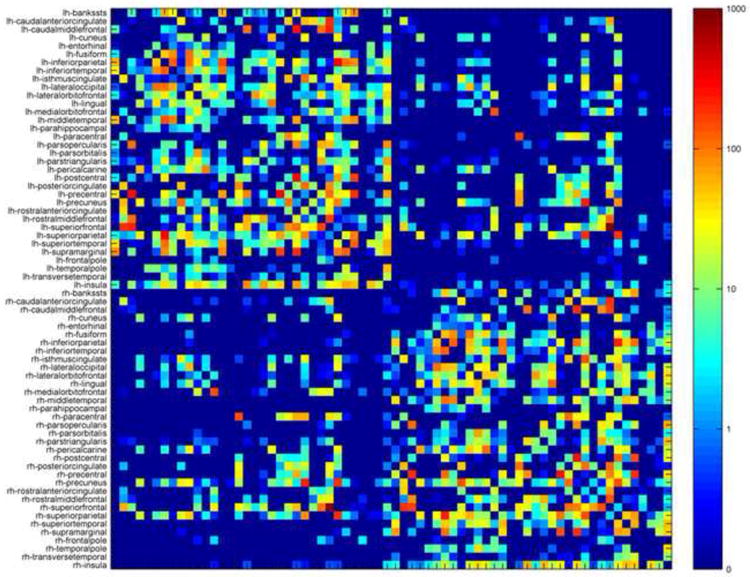
The average brain network connectivity matrix for the control group in this study. The elements of this matrix indicate the average numbers of fibers or streamlines connecting node pairs. Note that this matrix is symmetrical. The prefix lh and rh indicate nodes in the left and right hemispheres, respectively.
Calculated by averaging the graph distances of shortest paths between all pairs of nodes, the characteristic path length (CPL) (28) is commonly used to measure network integration (node-level path length is defined similarly by averaging the shortest paths connecting this node to all other nodes in the entire network). Networks with longer CPL exhibit information flows that are “impeded” or “slower” (due to the longer distance needed to travel between nodes) compared to those with shorter CPL, and are thus less efficient. A related global metric, the global efficiency (Eglob) calculates the average inverse shortest length between all pairs of nodes. Thus, both higher Eglob values and lower CPL values indicate more efficient networks.
Last, as a measure of network clustering or segregation, the weighted clustering coefficient (CC) (28) of a node is defined as the percentage of its neighbors that are also connected among themselves (nodes with high CC thus form locally interconnected clusters). The CC of the whole network averages CC across all nodes.
In this study, graph theory metrics were computed using Matlab functions implemented in the Brain Connectivity Toolbox (https://sites.google.com/a/brain-connectivity-toolbox.net/bct).
Measuring inter-modular integration
Given any pre-defined network community structure (a set of non-overlapping modules – e.g., the cerebrum can be considered a community with two modules: the cortical versus sub-cortical regions; Table 2 lists the 68 Freesurfer-derived cortical regions), the mean participation coefficients (29) has been proposed to measure the diversity of inter-modular connections for each node. Mathematically, it measures how well any particular node integrates with nodes in other modules. Thus, if a node only directly connects with nodes within the same module, its participation coefficient is 0.
Table 2.
Thirty-four Freesurfer-derived cortical labels per hemisphere extracted as the basis for our 68×68 cortical connectivity matrices used in the inter-hemispheric integration analysis (note that these do not include the additional 19 Freesurfer-derived subcortical gray matter regions).
| 1 | Banks of the superior temporal sulcus | 18 | Pars orbitalis |
| 2 | Caudal anterior cingulate | 19 | Pars triangularis |
| 3 | Caudal middle frontal | 20 | Peri-calcarine |
| 4 | Cuneus | 21 | Postcentral |
| 5 | Entorhinal | 22 | Posterior cingulate |
| 6 | Fusiform | 23 | Pre-central |
| 7 | Inferior parietal | 24 | Precuneus |
| 8 | Inferior temporal | 25 | Rostral anterior cingulate |
| 9 | Isthmus of the cingulate | 26 | Rostral middle frontal |
| 10 | Lateral occipital | 27 | Superior frontal |
| 11 | Lateral orbitofrontal | 28 | Superior parietal |
| 12 | Lingual | 29 | Superior temporal |
| 13 | Medial orbitofrontal | 30 | Supra-marginal |
| 14 | Middle temporal | 31 | Frontal pole |
| 15 | Parahippocampal | 32 | Temporal pole |
| 16 | Paracentral | 33 | Transverse temporal |
| 17 | Pars opercularis | 34 | Insula |
Additionally, we developed a set of four metrics to further probe modular integrations, which we term intra-/inter- modular path length and intra-/inter modular efficiency (intra-PL, inter-PL, Eintra, and Einter). The intra-PL (Eintra) is computed using the mean within-module path length (inverse path length), averaged across all shortest paths connecting node pairs in the same module. On the other hand, Inter-PL (Einter) is numerically defined as the mean inter-modular path length (inverse path length; see Appendix for mathematical formulae of CPL, Eglob and the proposed metrics).
Statistical analysis
Clinical and demographic data were analyzed using a one-way analysis of variance (ANOVA) for continuous variables and chi-squared test for categorical variables. Differences between groups on DTI measures and network metrics were determined using a one-way ANOVA with age, gender, and education as covariates.
3. Results
Demographics
The bipolar and control subjects did not differ in either gender or age. By contrast, control subjects received a significantly higher level of education than the bipolar group (education in years: 15.63 (±2.16) for control versus 14.00 (±1.63) for bipolar; t-statistic=2.98;df = 47 p=0.005). In the bipolar group, the mean total duration of illness at the time of the MRI scan was 20.80 ±13.96 (number of years since first depression was 18.50 ±15.46, and 14.96 ±12.73 since first mania). For DTI, there were no group differences in the total number of streamlines generated (58676±6461 in healthy; 55914±5612 in bipolar; p=0.12) or in head movement (the average head movements along x, y, and z directions for both groups were less than 0.5mm).
Whole brain white matter analyses
After controlling for multiple comparisons across all regions using Bonferroni correction at 0.05, the following regions exhibited statistically significant group differences in FA: the genu of corpus callosum (FA values 0.58 ±0.042 for control versus 0.54±0.051 for bipolar; F-statistic=18.4; p<0.001), the body of corpus callosum (0.64±0.036 for control versus 0.60±0.048 for bipolar; F-statistic=12.4; p=0.001), and the splenium of corpus callosum (0.69 ±0.029 for control versus 0.67±0.018 for bipolar; F-statistic=15.80; p<0.001). There was no significant group difference in MD for any white matter structure (before controlling for multiple comparisons, the genu exhibited higher MD values in the bipolar group at p=0.019).
Graph-theoretical structural network analyses
Results for path length (both global and node-level) and network efficiency are similar for both connectivity-to-length mappings. We will mainly present results based on the element-wise inverse mapping, and discuss relevant differences as indicated for the element-wise inverse square root mapping (note the computation of the remaining parameters do not depend on the choice of this mapping).
Global brain network analysis
Table 3 summarizes the global network analysis results using the element wise inverse mapping. After controlling for gender, age and education, the bipolar group globally exhibited significantly lower clustering coefficient (p=0.002, F=11.02), longer characteristic path length (for both connectivity-to-length mappings; p=0.014, F=6.57 for the element-wise inverse mapping and p=0.006, F=8.24 for the element-wise inverse square root mapping), and lower global efficiency (p<0.001, F = 14.92 for the element-wise inverse mapping; p=0.008, F=7.85 using the element-wise inverse square root mapping) relative to controls. By contrast, the two groups did not differ in network degree or density.
Table 3. Mean and standard deviation (SD) of global network metrics for the bipolar and healthy control subjects in this study (element-wise inverse mapping was used to calculate the characteristic path length and global efficiency).
| Value | F | df | P | ||
|---|---|---|---|---|---|
| Clustering coefficient | |||||
|
|
|||||
| Bipolar | 11.82±(1.100) | ||||
| Healthy controls | 12.59±(1.507) | 11.0 2 | 1,44 | 0.002 | |
|
|
|||||
| Characteristic path Length (using element-wise inverse mapping, see text) | |||||
|
|
|||||
| Bipolar | 0 .0 61± (0.013) | ||||
| Healthy controls | 0.055±(0.011) | 6.57 | 1,44 | 0.014 | |
|
|
|||||
| Degree | |||||
|
|
|||||
| Bipolar | 18.77± (1.324) | ||||
| Healthy controls | 19.07±(1.197) | ||||
| 1.31 6 | 1,44 | 0.258 | |||
|
|
|||||
| Eglobal (using element-wise inverse mapping) | |||||
|
|
|||||
| Bipolar | 33.03± (3.827) | ||||
| Healthy controls | 36.05±(4.496) | ||||
| 14.9 2 | 1,44 | <0.001 |
Node-level network analysis
Guided by our a priori hypotheses, we investigated node-level group differences in 20 ROIs (10 in each hemisphere) out of all 87 Freesurfer-derived regions. These ROIs are the bilateral orbito-frontal cortex (including medial and lateral orbitofrontal cortex), the cingulate (sub-divided into caudal-anterior, rostral-anterior, posterior, and isthmus) and temporal lobe limbic structures (amygdala, parahippocampal gyrus, hippocampus, and entorhinal cortex).
After controlling for age, gender and education, node-level network analyses for these ROIs using the element-wise inverse mapping are summarized in Table 4. Results show that bipolar subjects exhibited significantly lower clustering coefficient or longer node-level path length in sub-regions within the fronto-limbic circuitry (detailed node-level path length group differences using element-wise inverse square root mapping are summarized in the supplemental table S; overall the results showed similar patterns of group differences). After controlling for multiple comparisons (Bonferroni; cut-off p value at 0.05/20 =0.0025 for a total of 20 regions), group differences in the following regions remained significant with bipolar subjects exhibiting longer node-level path length: the left hippocampus, the left lateral orbito-frontal cortex, and the bilateral isthmus cingulate.
Table 4.
Mean and standard deviation (SD) of local node-level network metrics for the 20 frontolimbic ROIs (10 in each hemisphere) proposed in our a priori hypotheses. Only regions exhibiting significant group differences at p=0.05 (uncorrected) are shown (the element-wise inverse mapping was used to generate node-level path length).
| Clustering Coefficient | F | df | P | ||
|---|---|---|---|---|---|
| Hippocampus, left | |||||
|
|
|||||
| Bipolar | 6.37± (1.288) | ||||
| Healthy controls | 7.54± (1.885) | ||||
| 8.10 | 1,44 | 0.007 | |||
|
|
|||||
| Isthmus cingulate, right | |||||
|
|
|||||
| Bipolar | 7.84± (2.577) | ||||
| Healthy controls | 9.26± (1.947) | ||||
| 5.62 | 1,44 | 0.022 | |||
| Path Length | F | df | P | ||
|
| |||||
| Hippocampus, left | |||||
|
|
|||||
| Bipolar | 0.046± (0.008) | ||||
| Healthy controls | 0.041±(0.007) | ||||
| 12.5 | 1,44 | 0.001 | |||
|
|
|||||
| Hippocampus, right | |||||
|
|
|||||
| Bipolar | 0.046± (0.008) | ||||
| Healthy controls | 0.042± (0.007) | ||||
| 7.72 | 1,44 | 0.008 | |||
|
|
|||||
| Caudalanterior cingulate, left | |||||
|
|
|||||
| Bipolar | 0.042± (0.008) | ||||
| Healthy controls | 0.039± (0.007) | ||||
| 4.74 | 1,44 | 0.035 | |||
|
|
|||||
| Isthmus cingulate, left | |||||
|
|
|||||
| Bipolar | 0.054± (0.009) | ||||
| Healthy controls | 0.046± (0.009) | ||||
| 13.37 | 1,44 | 0.001 | |||
|
|
|||||
| Lateral orbitofrontal, left | |||||
|
|
|||||
| Bipolar | 0.048± (0.008) | ||||
| Healthy controls | 0.043± (0.007) | ||||
| 10.66 | 1,44 | 0.002 | |||
|
|
|||||
| Medial orbitofrontal, left | |||||
|
|
|||||
| Bipolar | 0.047± (0.008) | ||||
| Healthy controls | 0.044± (0.007) | ||||
| 6.12 | 1,44 | 0.017 | |||
|
|
|||||
| Parahippocampal, left | |||||
|
|
|||||
| Bipolar | 0.109± (0.039) | ||||
| Healthy controls | 0.087±(0.031) | ||||
| 5.32 | 1,44 | 0.026 | |||
|
|
|||||
| Caudalanterior cingulate, right | |||||
|
|
|||||
| Bipolar | 0.041±(0.007) | ||||
| Healthy controls | 0.038± (0.007) | ||||
| 4.46 | 1,44 | 0.040 | |||
|
|
|||||
| Isthmus cingulate, right | |||||
|
|
|||||
| Bipolar | 0.051±(0.008) | ||||
| Healthy controls | 0.042± (0.008) | ||||
| 23.8 | 1,44 | <0.001 | |||
|
|
|||||
| Lateral orbitofrontal, right | |||||
|
|
|||||
| Bipolar | 0.049± (0.008) | ||||
| Healthy controls | 0.045± (0.008) | ||||
| 7.51 | 1,44 | 0.009 | |||
|
|
|||||
| Medial orbitofrontal, right | |||||
|
|
|||||
| Bipolar | 0.045± (0.007) | ||||
| Healthy controls | 0.042± (0.008) | ||||
| 5.88 | 1,44 | 0.02 | |||
As exploratory analyses, in the bipolar group for all white matter integrity measures and graph-theoretical network measures (both global and nodal), partial correlations were computed with clinical features such as number of episodes and durations of illness controlling for age, gender, and education. None of the parameters exhibited significant correlations.
Investigating inter-hemispheric integration
Guided by the FA findings in the corpus callosum in the bipolar group, we thus further investigated relative abnormalities in intra-hemispheric versus inter-hemispheric network integration. As the corpus callosum anatomically connects bilateral cortical regions, we created a “left-right” community structure by dividing all Freesurfer-derived cortical regions into those in the left versus right hemisphere (34 cortical regions in each hemisphere, Table 2). To measure the integration of the left and right hemispheres, we first computed and compared, between groups, the mean participation coefficients for each hemisphere (by averaging the participation coefficients of all nodes within the same hemisphere), and found no significant group difference.
Next, we computed the proposed four new metrics (intra-PL, inter-PL, Eintra, and Einter) to further probe inter-hemispheric integration (here, the inter-PL for example, measures the mean path length when connecting any node to another node in the contralateral hemisphere and intra-PL in the ipsilateral hemisphere).
After controlling for multiple comparisons (Bonferroni corrections; cut-off p value at 0.05/12 for a total of 12 tests) results showed that bipolar subjects exhibited significantly attenuated inter-hemispheric integration (lower inter-hemispheric efficiency and longer inter-hemispheric path length) relative to control subjects when the element-wise inverse-square root transform is used (inter-hemispheric efficiency: 2.57 ±0.28 in bipolar versus 2.83±0.25 in control, F=17.4 and p<0.001; inter-hemispheric path length: 0.490±0.049 in bipolar versus 0.453±0.047 in control, F=13.03 and p=0.001), as well as significantly lower inter-hemispheric efficiency when the element-wise inverse mapping was applied (23.90±4.50 in bipolar versus 28.52±4.37 in control, F=20.86 and p<0.001). For intra-hemispheric path length/efficiency, significant differences were found only for Eintra in the right hemisphere (3.53±0.22 in bipolar versus 3.69±0.26 in control, F=13.25 and p=0.001, element-wise inverse square root mapping). These results are visualized in Figure 3.
Figure 3.
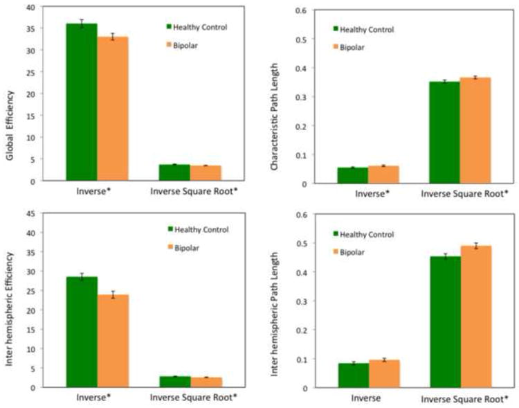
This figure shows group differences in global efficiency and characteristic path length (top panel), and inter-hemispheric efficiency and path length (lower panel) using both connectivity-to-length mappings.*indicates p < .05 (top row); p ≤ .001 (bottom row)
Lastly, post-hoc analyses (table 5) were conducted to further localize corpus callosal abnormalities in inter-hemispheric integration, by separately investigating inter-PL and Einter within the frontal, parietal, temporal, and occipital lobes. Results revealed widespread inter-hemispheric integration abnormalities with the most statistically significant deficit in the frontal lobe, thus suggesting prominent corpus callosal abnormality in the genu and anterior body.
Table 5.
Post-hoc analyses of inter-hemispheric integration in the frontal, temporal, parietal, and occipital lobes. This table shows the mean and standard deviation (SD) of lobar inter-hemispheric path length and efficiency (computed using both connectivity-to-length mappings). Only group differences reaching statistical significance are shown (Bonferroni correction with a total of 16 tests; cut-off p value 0.05/16=0.003)
| Element-wise inverse mapping | F | df | P | ||
|---|---|---|---|---|---|
| Inter-hemispheric path length Occipital lobe | |||||
|
|
|||||
| Bipolar | 0.054±(0.014) | ||||
| Healthy controls | 0.044±(0.010) | ||||
| 10.64 | 1,44 | 0.0021 | |||
|
|
|||||
| Inter-hemispheric efficiency Frontal lobe | |||||
|
|
|||||
| Bipolar | 22.9±(4.86) | ||||
| Healthy controls | 27.9±(6.26) | ||||
| 17.29 | 1,44 | 1.5×10⁻⁴ | |||
|
|
|||||
| Inter-hemispheric efficiency Temporal lobe | |||||
|
|
|||||
| Bipolar | 54.6±(17.9) | ||||
| Healthy controls | 71.4±(20.3) | ||||
| 11.27 | 1,44 | 0.0016 | |||
|
|
|||||
| Inter-hemispheric efficiency Occipital lobe | |||||
|
|
|||||
| Bipolar | 22.9±(4.86) | ||||
| Healthy controls | 27.9±(6.26) | ||||
| 10.38 | 1,44 | 0.0024 | |||
|
|
|||||
| Inter-hemispheric efficiency Parietal lobe | |||||
|
|
|||||
| Bipolar | 54.6±(17.9) | ||||
| Healthy controls | 71.4±(20.3) | ||||
| 9.87 | 1,44 | 0.0030 | |||
| Element-wise inverse square root mapping | F | df | P | ||
|
| |||||
| Inter-hemispheric path length Frontal lobe | |||||
|
|
|||||
| Bipolar | 0.40±(0.044) | ||||
| Healthy controls | 0.37±(0.037) | ||||
| 12.20 | 1,44 | 0.0011 | |||
|
|
|||||
| Inter-hemispheric path length Occipital lobe | |||||
|
|
|||||
| Bipolar | 0.36±(0.055) | ||||
| Healthy controls | 0.32±(0.040) | ||||
| 10.66 | 1,44 | 0.0021 | |||
|
|
|||||
| Inter-hemispheric Efficiency Frontal lobe | |||||
|
|
|||||
| Bipolar | 3.49±(0.46) | ||||
| Healthy controls | 3.86±(0.37) | ||||
| 15.62 | 1,44 | 2.8×10⁻⁴ | |||
|
|
|||||
| Inter-hemispheric Efficiency Temporal lobe | |||||
|
|
|||||
| Bipolar | 1.60±(0.17) | ||||
| Healthy controls | 1.73±(0.21) | ||||
| 11.79 | 1,44 | 0.0013 | |||
4. Discussion
In this study, we acquired and analyzed 64-direction diffusion-weighted MR imaging data in a sample of 25 bipolar and 24 age/gender matched subjects, and conducted whole brain white matter integrity analyses. Additionally, this represents, to our knowledge, the first brain network analysis study in euthymic bipolar subjects.
Our whole brain white matter analyses results revealed abnormal white matter integrity in the corpus callosum. These findings support the possibility that white matter integrity abnormalities in bipolar disorder may be a result of abnormal oligodendrocyte function and/or impaired integrity of the myelin sheath.
Structural brain network analyses further revealed that, on a global level, bipolar subjects exhibit longer characteristic path length, lower clustering coefficient, and lower global efficiency compared to controls, suggesting impaired global integration in bipolar disorder. Such group differences could not be explained by an overall decrease in the number of total reconstructed fibers or lower densities in the connectivity matrices of bipolar subjects, as the two groups did not significantly differ in either.
Guided by the corpus callosum findings in white matter analyses, we further devised novel metrics to probe and compare intra- versus inter-hemispheric integration. These revealed relative deficits in inter-hemispheric integration in bipolar subjects compared to healthy controls. Post-hoc analyses revealed that integration deficits were statistically most significant between the bilateral frontal lobes, although there was evidence of widespread deficits in the temporal, parietal, and occipital lobes (Table 5; also note that in the white matter integrity analyses, we found lower FA in all sub-divisions of the corpus callosum). These results thus localized most prominent inter-hemispheric integration deficits to the anterior section of the corpus callosum (i.e., genu and anterior body).
Subsequent local network analyses revealed node-level longer path length in the left hippocampus, the left lateral orbitofrontal cortex, and the bilateral isthmus cingulate. These results are consistent with previous findings of disruptions along tracts connecting orbitofrontal cortex and amygdala/hippocampus in bipolar disorder (1). An important tract connecting these regions, the left uncinate fasciculus exhibited lower FA values in the bipolar subjects in our whole brain white matter analysis, although such group differences did not reach statistical significance. Additionally, the observed longer node-level path length in the bilateral isthmus cingulate may suggest disruptions in the Papez circuit. As an important component of this circuit, the cingulate projects (via the cingulum) to the parahippocampus, which in turn projects to the hippocampus.
Contrary to our findings of globally less efficient (longer path length) and locally less clustered brain networks in subjects with bipolar disorder, a recent study on first-episode unipolar major depressive disorder (31) using functional connectivity-based brain network analyses reported shorter path length and higher global efficiency in the depressed group (with localizations to the caudate and to default mode network regions). These divergent results strongly suggest different underlying pathophysiologies between unipolar depression and bipolar disorder (for a review of structural MRI findings in major depression versus bipolar disorder, we refer the readers to (32)).
Our results may have significant clinical implications. In this study, we found lower left-right hemispheric integration. This observed left-right dis-integration adds another layer of complexity to the possible role of brain asymmetry in the pathophysiology of mood disorders. For decades, asymmetrical effects have been observed in numerous studies of affective disorders (33, 34). Unilateral left hemispheric hypometabolism has been observed in depressed patients (35, 36). By contrast, patients with primary mania have demonstrated lower perfusion on SPECT images, in the right versus left basal temporal cortex, suggesting that the right basotemporal cortex may be involved in regulating the production of primary mania (37). Also, when applied to the left prefrontal cortex, transcranial magnetic stimulation can offer therapeutic effects in drug-resistant depression (38, 39). Additionally, pre-existing anatomical asymmetries are also thought to interact with the severity of depressive symptoms in patients with cerebral lesions (40). In another interesting but less known study assessing perceptual shifts and binocular rivalry (41), the authors suggested that in bipolar disorder hemispheric activation may be resistant to the normal process of switching. They thus offered a theory that bipolar disorder may result from a genetic propensity for slow interhemispheric switching mechanisms that become persistent in one or the other state.
Our study has several strengths. We studied a well characterized group of bipolar I subjects in the euthymic state, while several prior DTI studies have combined both bipolar I and II or have studied subjects in different mood states (9, 14, 17, 18, 42-45). These variables could confound findings and add to the heterogeneity of DTI results reported thus far.
However, this study has its limitations. Although an exciting and novel technological advance in neuroimaging, diffusion tractography has its own limitations (e.g., spurious streamlines may exist that are not supported by evidence), a full discussion of which we refer to in (46). Moreover, brain network analyses have been shown to be dependent on the streamline reconstruction technique (47), the choice of neuro-anatomical atlases (i.e., the definition of the “nodes”) (48, 49), and different matrix normalization strategies (50). Also, in this study we used 12-parameter affine transformations for realigning the MPRAGE and DTI spaces, which only incompletely corrects for B0 inhomogeneity-induced geometric distortions. More sophisticated and computationally involved treatment (e.g.,(51)) using highly non-linear registration techniques may be better suited for the rigorous correction for any such distortions. Lastly, due to the heterogeneous medication profile of our sample and the fact that only two of our study participants were medication free at the time of the study, medication effects could not be fully explored.
The possible dependence of brain structural and functional abnormalities on mood states and medications merits additional discussion. For example, it has been speculated that FA may be increased in the euthymic state, while in depression lower FA has been more consistently observed (9, 14, 17, 18, 42-45). In the current study, mood was not a confound in that all bipolar subjects were euthymic.
Although the dependence of white matter structural integrity on medications is less investigated, one study has reported medication load-associated lower FA values in the left optic radiation and right antero-thalamic radiation in subjects with bipolar disorder (16). In addition, there is evidence of medication effects in volumetric MRI studies in bipolar disorder. For example, (52) found that the subgenual prefrontal cortex was 40% smaller in unmedicated bipolar patients than in controls. However, patients treated with lithium or valproate were not significantly different from controls, and had significantly higher subgenual prefrontal cortex volumes than unmedicated patients. In two related studies (53, 54), larger hippocampal volumes were found in subjects treated with lithium. A recent meta-analysis of 98 structural imaging studies of bipolar disorder found that lithium use was associated with significantly increased total gray matter volume across studies (55). Further supporting these findings, in other areas of neuroscience research lithium has been suggested to be neuro-protective (56) and may exert this property by regulating several cyto-protective pathways (57).
Another possible limitation of this study is the sample size. Our sample size may not have been powered to detect differences in intra-hemispheric integration, for which there was some evidence of group differences (lower level of integration in bipolar relative to control subjects).
4. Conclusion
This study represents the first brain network analyses in bipolar disorder. Results revealed persistent white matter abnormalities in euthymic bipolar patients in the corpus callosum. Abnormal inter-hemispheric integration, as shown by brain network analyses, further supports the possibility that these abnormalities of the corpus callosum may contribute to disturbed brain network organization, particularly in fronto-limbic regions, in bipolar disorder.
Supplementary Material
Figure S. The brain network distance matrix from a normal control subject in this study. The elements of this matrix indicate the shortest weighted path length connecting node pairs. Only the upper-diagonal part is shown, as the matrix is symmetrical. In this example, the element-wise inverse of the element-wise square root mapping is used. The prefix lh and rh indicate nodes in the left and right hemispheres, respectively. The area outlined in red denotes inter-hemispheric connections.
Table S. Mean and standard deviation (SD) of node-level path lengths for the 20 fronto-limbic ROIs proposed in our a priori hypotheses. Here, node-level path length was computed using the element-wise inverse square root connectivity-to-length mapping. Only regions reaching statistical significance (uncorrected) are shown.
In this issue statement.
We acquired diffusion-weighted MRI on 25 bipolar I subjects and 24 gender and age equivalent healthy controls. We investigated white matter integrity in the whole brain, and conducted first ever brain network analyses in bipolar disorder using a graph-theoretical approach.
Our results revealed that bipolar brain networks exhibited lower local clustering and global efficiency relative to those of controls. Further analyses suggested significantly impaired inter-hemispheric integration in the bipolar group.
Footnotes
Conflict of Interests: The authors have no conflict of interests to report.
References
- 1.Mahon K, Burdick KE, Szeszko PR. A role for white matter abnormalities in the pathophysiology of bipolar disorder. Neuroscience and biobehavioral reviews. 2010;34:533–554. doi: 10.1016/j.neubiorev.2009.10.012. [DOI] [PMC free article] [PubMed] [Google Scholar]
- 2.Tkachev D, Mimmack ML, Ryan MM, Wayland M, Freeman T, Jones PB, et al. Oligodendrocyte dysfunction in schizophrenia and bipolar disorder. Lancet. 2003;362:798–805. doi: 10.1016/S0140-6736(03)14289-4. [DOI] [PubMed] [Google Scholar]
- 3.Regenold WT, Phatak P, Marano CM, Gearhart L, Viens CH, Hisley KC. Myelin staining of deep white matter in the dorsolateral prefrontal cortex in schizophrenia, bipolar disorder, and unipolar major depression. Psychiatry Res. 2007;151:179–188. doi: 10.1016/j.psychres.2006.12.019. [DOI] [PubMed] [Google Scholar]
- 4.Beyer JL, Taylor WD, MacFall JR, Kuchibhatla M, Payne ME, Provenzale JM, et al. Cortical white matter microstructural abnormalities in bipolar disorder. Neuropsychopharmacology. 2005;30:2225–2229. doi: 10.1038/sj.npp.1300802. [DOI] [PubMed] [Google Scholar]
- 5.Kafantaris V, Kingsley P, Ardekani B, Saito E, Lencz T, Lim K, et al. Lower orbital frontal white matter integrity in adolescents with bipolar I disorder. J Am Acad Child Adolesc Psychiatry. 2009;48:79–86. doi: 10.1097/CHI.0b013e3181900421. [DOI] [PMC free article] [PubMed] [Google Scholar]
- 6.Benedetti F, Absinta M, Rocca MA, Radaelli D, Poletti S, Bernasconi A, et al. Tract-specific white matter structural disruption in patients with bipolar disorder. Bipolar Disord. 2011;13:414–424. doi: 10.1111/j.1399-5618.2011.00938.x. [DOI] [PubMed] [Google Scholar]
- 7.Bellani M, Yeh PH, Tansella M, Balestrieri M, Soares JC, Brambilla P. DTI studies of corpus callosum in bipolar disorder. Biochem Soc Trans. 2009;37:1096–1098. doi: 10.1042/BST0371096. [DOI] [PubMed] [Google Scholar]
- 8.Heng S, Song AW, Sim K. White matter abnormalities in bipolar disorder: insights from diffusion tensor imaging studies. J Neural Transm. 2010;117:639–654. doi: 10.1007/s00702-010-0368-9. [DOI] [PubMed] [Google Scholar]
- 9.Benedetti F, Yeh PH, Bellani M, Radaelli D, Nicoletti MA, Poletti S, et al. Disruption of white matter integrity in bipolar depression as a possible structural marker of illness. Biol Psychiatry. 2011;69:309–317. doi: 10.1016/j.biopsych.2010.07.028. [DOI] [PubMed] [Google Scholar]
- 10.Adler CM, Adams J, DelBello MP, Holland SK, Schmithorst V, Levine A, et al. Evidence of white matter pathology in bipolar disorder adolescents experiencing their first episode of mania: a diffusion tensor imaging study. Am J Psychiatry. 2006;163:322–324. doi: 10.1176/appi.ajp.163.2.322. [DOI] [PubMed] [Google Scholar]
- 11.Adler CM, Holland SK, Schmithorst V, Wilke M, Weiss KL, Pan H, et al. Abnormal frontal white matter tracts in bipolar disorder: a diffusion tensor imaging study. Bipolar Disord. 2004;6:197–203. doi: 10.1111/j.1399-5618.2004.00108.x. [DOI] [PubMed] [Google Scholar]
- 12.Bruno S, Cercignani M, Ron MA. White matter abnormalities in bipolar disorder: a voxel-based diffusion tensor imaging study. Bipolar Disord. 2008;10:460–468. doi: 10.1111/j.1399-5618.2007.00552.x. [DOI] [PMC free article] [PubMed] [Google Scholar]
- 13.Frazier JA, Breeze JL, Papadimitriou G, Kennedy DN, Hodge SM, Moore CM, et al. White matter abnormalities in children with and at risk for bipolar disorder. Bipolar Disord. 2007;9:799–809. doi: 10.1111/j.1399-5618.2007.00482.x. [DOI] [PubMed] [Google Scholar]
- 14.Yurgelun-Todd DA, Silveri MM, Gruber SA, Rohan ML, Pimentel PJ. White matter abnormalities observed in bipolar disorder: a diffusion tensor imaging study. Bipolar Disord. 2007;9:504–512. doi: 10.1111/j.1399-5618.2007.00395.x. [DOI] [PubMed] [Google Scholar]
- 15.Mahon K, Wu J, Malhotra AK, Burdick KE, DeRosse P, Ardekani BA, et al. A voxel-based diffusion tensor imaging study of white matter in bipolar disorder. Neuropsychopharmacology. 2009;34:1590–1600. doi: 10.1038/npp.2008.216. [DOI] [PMC free article] [PubMed] [Google Scholar]
- 16.Versace A, Almeida JR, Hassel S, Walsh ND, Novelli M, Klein CR, et al. Elevated left and reduced right orbitomedial prefrontal fractional anisotropy in adults with bipolar disorder revealed by tract-based spatial statistics. Arch Gen Psychiatry. 2008;65:1041–1052. doi: 10.1001/archpsyc.65.9.1041. [DOI] [PMC free article] [PubMed] [Google Scholar]
- 17.Haznedar MM, Roversi F, Pallanti S, Baldini-Rossi N, Schnur DB, Licalzi EM, et al. Fronto-thalamo-striatal gray and white matter volumes and anisotropy of their connections in bipolar spectrum illnesses. Biol Psychiatry. 2005;57:733–742. doi: 10.1016/j.biopsych.2005.01.002. [DOI] [PubMed] [Google Scholar]
- 18.Sussmann JE, Lymer GK, McKirdy J, Moorhead TW, Munoz Maniega S, Job D, et al. White matter abnormalities in bipolar disorder and schizophrenia detected using diffusion tensor magnetic resonance imaging. Bipolar Disord. 2009;11:11–18. doi: 10.1111/j.1399-5618.2008.00646.x. [DOI] [PubMed] [Google Scholar]
- 19.Barnea-Goraly N, Chang KD, Karchemskiy A, Howe ME, Reiss AL. Limbic and corpus callosum aberrations in adolescents with bipolar disorder: a tract-based spatial statistics analysis. Biol Psychiatry. 2009;66:238–244. doi: 10.1016/j.biopsych.2009.02.025. [DOI] [PubMed] [Google Scholar]
- 20.Wang F, Jackowski M, Kalmar JH, Chepenik LG, Tie K, Qiu M, et al. Abnormal anterior cingulum integrity in bipolar disorder determined through diffusion tensor imaging. Br J Psychiatry. 2008;193:126–129. doi: 10.1192/bjp.bp.107.048793. [DOI] [PMC free article] [PubMed] [Google Scholar]
- 21.Bassett DS, Brown JA, Deshpande V, Carlson JM, Grafton ST. Conserved and variable architecture of human white matter connectivity. Neuroimage. 2011;54:1262–1279. doi: 10.1016/j.neuroimage.2010.09.006. [DOI] [PubMed] [Google Scholar]
- 22.Bullmore E, Sporns O. Complex brain networks: graph theoretical analysis of structural and functional systems. Nat Rev Neurosci. 2009;10:186–198. doi: 10.1038/nrn2575. [DOI] [PubMed] [Google Scholar]
- 23.Rubinov M, Sporns O. Complex network measures of brain connectivity: uses and interpretations. NeuroImage. 2010;52:1059–1069. doi: 10.1016/j.neuroimage.2009.10.003. [DOI] [PubMed] [Google Scholar]
- 24.Iturria-Medina Y, Sotero RC, Canales-Rodriguez EJ, Aleman-Gomez Y, Melie-Garcia L. Studying the human brain anatomical network via diffusion-weighted MRI and Graph Theory. Neuroimage. 2008;40:1064–1076. doi: 10.1016/j.neuroimage.2007.10.060. [DOI] [PubMed] [Google Scholar]
- 25.Young RC, Biggs JT, Ziegler VE, Meyer DA. A rating scale for mania: reliability, validity and sensitivity. Br J Psychiatry. 1978;133:429–435. doi: 10.1192/bjp.133.5.429. [DOI] [PubMed] [Google Scholar]
- 26.Hamilton M. Rating depressive patients. J Clin Psychiatry. 1980;41:21–24. [PubMed] [Google Scholar]
- 27.Dijkstra EW. A note on two problems in connexion with graphs. Numerische Mathematik. 1959;1:269–271. [Google Scholar]
- 28.Watts DJ, Strogatz SH. Collective dynamics of ‘small-world’ networks. Nature. 1998;393:440–442. doi: 10.1038/30918. [DOI] [PubMed] [Google Scholar]
- 29.Guimera R, Nunes Amaral LA. Functional cartography of complex metabolic networks. Nature. 2005;433:895–900. doi: 10.1038/nature03288. [DOI] [PMC free article] [PubMed] [Google Scholar]
- 30.Benjamini Y. Controlling the false discovery rate: a practical and powerful approach to multiple testing. Journal of the Royal Statistical Society, Series B (Methodological) 1995;57(1):289–300. [Google Scholar]
- 31.Zhang J, Wang J, Wu Q, Kuang W, Huang X, He Y, et al. Disrupted brain connectivity networks in drug-naive, first-episode major depressive disorder. Biol Psychiatry. 2011;70:334–342. doi: 10.1016/j.biopsych.2011.05.018. [DOI] [PubMed] [Google Scholar]
- 32.Kempton MJ, Salvador Z, Munafo MR, Geddes JR, Simmons A, Frangou S, et al. Structural neuroimaging studies in major depressive disorder. Meta-analysis and comparison with bipolar disorder. Arch Gen Psychiatry. 2011;68:675–690. doi: 10.1001/archgenpsychiatry.2011.60. [DOI] [PubMed] [Google Scholar]
- 33.Davidson R. Brain asymmetry. MIT Press; London: 1995. [Google Scholar]
- 34.Kinsbourne M. Cerebral hemisphere function in depression. American Psychiatric Press, Inc; Washington: 1988. [Google Scholar]
- 35.Martinot JL, Hardy P, Feline A, Huret JD, Mazoyer B, Attar-Levy D, et al. Left prefrontal glucose hypometabolism in the depressed state: a confirmation. Am J Psychiatry. 1990;147:1313–1317. doi: 10.1176/ajp.147.10.1313. [DOI] [PubMed] [Google Scholar]
- 36.Bench CJ, Frackowiak RS, Dolan RJ. Changes in regional cerebral blood flow on recovery from depression. Psychol Med. 1995;25:247–261. doi: 10.1017/s0033291700036151. [DOI] [PubMed] [Google Scholar]
- 37.Migliorelli R, Starkstein SE, Teson A, de Quiros G, Vazquez S, Leiguarda R, et al. SPECT findings in patients with primary mania. J Neuropsychiatry Clin Neurosci. 1993;5:379–383. doi: 10.1176/jnp.5.4.379. [DOI] [PubMed] [Google Scholar]
- 38.Pascual-Leone A, Rubio B, Pallardo F, Catala MD. Rapid-rate transcranial magnetic stimulation of left dorsolateral prefrontal cortex in drug-resistant depression. Lancet. 1996;348:233–237. doi: 10.1016/s0140-6736(96)01219-6. [DOI] [PubMed] [Google Scholar]
- 39.George MS, Wassermann EM, Kimbrell TA, Little JT, Williams WE, Danielson AL, et al. Mood improvement following daily left prefrontal repetitive transcranial magnetic stimulation in patients with depression: a placebo-controlled crossover trial. Am J Psychiatry. 1997;154:1752–1756. doi: 10.1176/ajp.154.12.1752. [DOI] [PubMed] [Google Scholar]
- 40.Starkstein SE, Bryer JB, Berthier ML, Cohen B, Price TR, Robinson RG. Depression after stroke: the importance of cerebral hemisphere asymmetries. J Neuropsychiatry Clin Neurosci. 1991;3:276–285. doi: 10.1176/jnp.3.3.276. [DOI] [PubMed] [Google Scholar]
- 41.Pettigrew JD, Miller SM. A ‘sticky’ interhemispheric switch in bipolar disorder? Proc Biol Sci. 1998;265:2141–2148. doi: 10.1098/rspb.1998.0551. [DOI] [PMC free article] [PubMed] [Google Scholar]
- 42.Chaddock CA, Barker GJ, Marshall N, Schulze K, Hall MH, Fern A, et al. White matter microstructural impairments and genetic liability to familial bipolar I disorder. Br J Psychiatry. 2009;194:527–534. doi: 10.1192/bjp.bp.107.047498. [DOI] [PubMed] [Google Scholar]
- 43.Regenold WT, D'Agostino CA, Ramesh N, Hasnain M, Roys S, Gullapalli RP. Diffusion-weighted magnetic resonance imaging of white matter in bipolar disorder: a pilot study. Bipolar Disord. 2006;8:188–195. doi: 10.1111/j.1399-5618.2006.00281.x. [DOI] [PubMed] [Google Scholar]
- 44.Wessa M, Houenou J, Leboyer M, Chanraud S, Poupon C, Martinot JL, et al. Microstructural white matter changes in euthymic bipolar patients: a whole-brain diffusion tensor imaging study. Bipolar Disord. 2009;11:504–514. doi: 10.1111/j.1399-5618.2009.00718.x. [DOI] [PubMed] [Google Scholar]
- 45.Zanetti MV, Jackowski MP, Versace A, Almeida JR, Hassel S, Duran FL, et al. State-dependent microstructural white matter changes in bipolar I depression. Eur Arch Psychiatry Clin Neurosci. 2009;259:316–328. doi: 10.1007/s00406-009-0002-8. [DOI] [PMC free article] [PubMed] [Google Scholar]
- 46.Jbabdi S, Johansen-Berg H. Tractography: where do we go from here? Brain Connect. 2011;1:169–183. doi: 10.1089/brain.2011.0033. [DOI] [PMC free article] [PubMed] [Google Scholar]
- 47.Li L, Rilling JK, Preuss TM, Glasser MF, Hu X. The effects of connection reconstruction method on the interregional connectivity of brain networks via diffusion tractography. Human brain mapping. 2011 doi: 10.1002/hbm.21332. [DOI] [PMC free article] [PubMed] [Google Scholar]
- 48.Wang J, Wang L, Zang Y, Yang H, Tang H, Gong Q, et al. Parcellation-dependent small-world brain functional networks: a resting-state fMRI study. Hum Brain Mapp. 2009;30:1511–1523. doi: 10.1002/hbm.20623. [DOI] [PMC free article] [PubMed] [Google Scholar]
- 49.Zalesky A, Fornito A, Harding IH, Cocchi L, Yucel M, Pantelis C, et al. Whole-brain anatomical networks: does the choice of nodes matter? Neuroimage. 2010;50:970–983. doi: 10.1016/j.neuroimage.2009.12.027. [DOI] [PubMed] [Google Scholar]
- 50.van den Heuvel MP, Sporns O. Rich-club organization of the human connectome. The Journal of neuroscience : the official journal of the Society for Neuroscience. 2011;31:15775–15786. doi: 10.1523/JNEUROSCI.3539-11.2011. [DOI] [PMC free article] [PubMed] [Google Scholar]
- 51.Huang H, Ceritoglu C, Li X, Qiu A, Miller MI, van Zijl PC, et al. Correction of B0 susceptibility induced distortion in diffusion-weighted images using large-deformation diffeomorphic metric mapping. Magnetic resonance imaging. 2008;26:1294–1302. doi: 10.1016/j.mri.2008.03.005. [DOI] [PMC free article] [PubMed] [Google Scholar]
- 52.Drevets WC, Price JL, Simpson JR, Jr, Todd RD, Reich T, Vannier M, et al. Subgenual prefrontal cortex abnormalities in mood disorders. Nature. 1997;386:824–827. doi: 10.1038/386824a0. [DOI] [PubMed] [Google Scholar]
- 53.Yucel K, Taylor VH, McKinnon MC, Macdonald K, Alda M, Young LT, et al. Bilateral hippocampal volume increase in patients with bipolar disorder and short-term lithium treatment. Neuropsychopharmacology. 2008;33:361–367. doi: 10.1038/sj.npp.1301405. [DOI] [PubMed] [Google Scholar]
- 54.Bearden CE, Thompson PM, Dutton RA, Frey BN, Peluso MA, Nicoletti M, et al. Three-dimensional mapping of hippocampal anatomy in unmedicated and lithium-treated patients with bipolar disorder. Neuropsychopharmacology. 2008;33:1229–1238. doi: 10.1038/sj.npp.1301507. [DOI] [PMC free article] [PubMed] [Google Scholar]
- 55.Kempton MJ, Geddes JR, Ettinger U, Williams SC, Grasby PM. Meta-analysis, database, and meta-regression of 98 structural imaging studies in bipolar disorder. Arch Gen Psychiatry. 2008;65:1017–1032. doi: 10.1001/archpsyc.65.9.1017. [DOI] [PubMed] [Google Scholar]
- 56.Chuang DM, Manji HK. In search of the Holy Grail for the treatment of neurodegenerative disorders: has a simple cation been overlooked? Biol Psychiatry. 2007;62:4–6. doi: 10.1016/j.biopsych.2007.04.008. [DOI] [PMC free article] [PubMed] [Google Scholar]
- 57.Manji HK, Moore GJ, Chen G. Clinical and preclinical evidence for the neurotrophic effects of mood stabilizers: implications for the pathophysiology and treatment of manic-depressive illness. Biol Psychiatry. 2000;48:740–754. doi: 10.1016/s0006-3223(00)00979-3. [DOI] [PubMed] [Google Scholar]
Associated Data
This section collects any data citations, data availability statements, or supplementary materials included in this article.
Supplementary Materials
Figure S. The brain network distance matrix from a normal control subject in this study. The elements of this matrix indicate the shortest weighted path length connecting node pairs. Only the upper-diagonal part is shown, as the matrix is symmetrical. In this example, the element-wise inverse of the element-wise square root mapping is used. The prefix lh and rh indicate nodes in the left and right hemispheres, respectively. The area outlined in red denotes inter-hemispheric connections.
Table S. Mean and standard deviation (SD) of node-level path lengths for the 20 fronto-limbic ROIs proposed in our a priori hypotheses. Here, node-level path length was computed using the element-wise inverse square root connectivity-to-length mapping. Only regions reaching statistical significance (uncorrected) are shown.