Identifying the Neuroanatomical Basis of Cognitive Impairment in Alzheimer’s Disease by Correlation- and Nonlinearity-Aware Sparse Bayesian Learning

Abstract

Predicting cognitive performance of subjects from their magnetic resonance imaging (MRI) measures and identifying relevant imaging biomarkers are important research topics in the study of Alzheimer’s disease (AD). Traditionally, this task is performed by formulating a linear regression problem. Recently, it is found that using a linear sparse regression model can achieve better prediction accuracy. However, most existing studies only focus on the exploitation of sparsity of regression coefficients, ignoring useful structure information in regression coefficients. Also, these linear sparse models may not capture more complicated and possibly nonlinear relationships between cognitive performance and MRI measures. Motivated by these observations, in this work we build a sparse multivariate regression model for this task and propose an empirical sparse Bayesian learning algorithm. Different from existing sparse algorithms, the proposed algorithm models the response as a nonlinear function of the predictors by extending the predictor matrix with block structures. Further, it exploits not only inter-vector correlation among regression coefficient vectors, but also intra-block correlation in each regression coefficient vector. Experiments on the Alzheimer’s Disease Neuroimaging Initiative database showed that the proposed algorithm not only achieved better prediction performance than state-of-the-art competitive methods, but also effectively identified biologically meaningful patterns.

I. Introduction

Alzheimer’s disease (AD) is a neurodegenerative disorder characterized by progressive impairment of memory and other cognitive functions, associated with behavioral disturbances, and progressively leads to total dependency [1]. Identifying the neuroanatomical basis of cognitive impairment in AD is an important research topic because it can help us understand brain structural changes related to cognitive impairment and potentially predict the progression of AD [2]–[5].

This work considers the task of predicting cognitive scores of subjects from their magnetic resonance imaging (MRI) measures by identifying neuroimaging predictors for cognitive decline in AD. Increasing attention has been received in this field, where sparse learning methods are used to identify imaging biomarkers associated with cognitive, genetic or diagnostic conditions (e.g., [6]–[19]). For example, Stonnington et al. [6] applied relevance vector regression, a sparse kernel method formulated in a Bayesian framework, to the prediction of four sets of cognitive scores using the MRI voxel-based morphometry (VBM) measures. Nunea et al. [16] used Lasso and Elastic Net enhanced by bootstrap to select biomarkers. Sabuncu et al. [13] presented a Bayesian model utilizing sparse and spatially connected sets of voxels to predict age and AD diagnosis. These studies typically considered only the sparsity of the regression coefficients, ignoring other structures in the data. Wang et al. [9] and Zhang et al. [11] employed multi-task learning strategies for selecting biomarkers that could predict multiple clinical scores, using ℓ_2,1-norm coupled with ℓ₁-norm [9] and multi-task feature selection coupled with support vector machine [11], respectively. Both methods used a simple concatenation to bundle multiple clinical scores together without learning their correlation structure.

Two important issues are ignored in these studies. One issue is that all these sparsity-based methods considered linear sparse models, in which the response (e.g. cognitive score) is a linear function of predictors (e.g. neuroimaging measures). Although linear models showed promising results, modeling cognitive scores as nonlinear functions of neuroimaging measures provides enhanced flexibility and the potential to better capture the complex relationship between the two quantities.

The second issue is that most existing sparsity-based models only considered the sparsity of regression coefficients without modeling the correlation among the coefficients. In our case, for a cognitive test that produces multiple scores, a relevant imaging predictor typically has more or less influence on all these scores, which results in correlation among regression coefficients [10]. Zhang and Rao [20], [21] recently showed that exploiting such correlation could significantly improve algorithms’ performance. For a univariate sparse linear model, they showed that if the regression coefficient vector has block-sparse structure (namely, the nonzero entries in the vector cluster into a number of nonzero blocks), exploiting the correlation among entries in a common nonzero block (i.e., intra-block correlation) is greatly beneficial in finding the correct solution [21]. For a multivariate sparse linear model that involves multiple-outputs and estimates a coefficient matrix corresponding to multiple measurement vectors, they also showed that exploiting the correlation among different regression coefficient vectors (i.e., inter-vector correlation) can significantly reduce regression errors [20]. The benefit was also revealed in our previous work [10], in which we proposed a sparse Bayesian multi-task learning algorithm which explicitly models the correlation structure within each row of the regression coefficient matrix, i.e., inter-vector correlation, and achieved good prediction performance in predicting cognitive scores from imaging measures. However, to the best of our knowledge, there is no sparsity-based algorithm exploiting both the inter-vector and the intra-block correlation.

To bridge the gap, we propose a multivariate sparse regression model which possesses both the intra-block correlation and the inter-vector correlation in the regression coefficient matrix. We also present an approach to model the response as a nonlinear function of the predictors. A sparse Bayesian learning algorithm is derived, which estimates the solution by exploiting the sparsity of regression coefficients and automatically learning the intra-block and inter-vector correlations. Our main contribution can be summarized as follows.

From the perspective of our application, we provide a flexible framework to exploit the nonlinear relationship between cognitive scores and MRI measures. Although in this work we adopt a specific nonlinear function (i.e., a polynomial function), other nonlinear functions can also be used. We show that exploiting the two kinds of correlations can significantly improve the prediction performance and help accurately identify biologically meaningful imaging predictors. It is worth noting that exploiting nonlinearity and correlation is rare in neuroimaging research using sparse learning methods.

From the perspective of sparse regression algorithms, the proposed algorithm is the first sparse algorithm exploiting both the intra-block correlation and the inter-vector correlation, and it enriches the family of sparse Bayesian learning algorithms [22]. An efficient approach to learning the two correlation structures and a regularization approach for the associated covariance matrices are proposed. Besides, the algorithm is self-tuning, which is an obvious advantage to many sparse regression algorithms such as the Lasso-type algorithms which require users to tune some parameters via cross-validation.

II. Notations

Bold symbols are reserved for vectors and matrices. For a matrix A, A_i· denotes the i-th row, and A_·j denotes the j-th column. A_[i]j denotes the i-th block in the j-th column. A_i[j] denotes the j-th block in the i-th row. A_[i]· denotes the i-th block of all the columns, while A_·[j] denotes the j-th block of all the rows. A_[k] denotes the k-th diagonal block in A. diag{A₁, ···, A_M} denotes a block diagonal matrix with principal diagonal blocks being A₁, ···, A_M in turn. vec(A) denotes the vectorization of the matrix A formed by stacking its columns into a single column vector. ⊗ indicates the Kronecker product. A^T is the transpose of A.

III. Mathematical Model

Consider the multivariate linear regression model:

$$\mathbf{Y}=\mathbf{\Phi }\mathbf{X}+\mathbf{V}$$ (1)

where Y ∈ ℝ^M×L is the response matrix, X ∈ ℝ^N×L is the regression coefficient matrix, and V is the noise matrix. Φ ∈ ℝ^M×N is the predictor matrix, and any M columns are linearly independent. Further, the matrix X is assumed to have the following block structure:

$$\mathbf{X}=\left[\begin{array}{c}{\mathbf{X}}_{[1]·}\\ {\mathbf{X}}_{[2]·}\\ ⋮\\ {\mathbf{X}}_{[g]·}\end{array}\right]$$ (2)

where X_[i]· ∈ ℝ^d_i×L is the i-th block of X, and ${\sum }_{i=1}^g{d}_i=N$. Among the g blocks, only a few are nonzero blocks. The key assumption in this model is that each block X_[i]·(∀i) is assumed to have both intra-block correlation and inter-vector correlation. In particular, entries in the same column of X_[i]· are correlated (intra-block correlation), and entries in the same row of X_[i]· are also correlated (inter-vector correlation).

To facilitate algorithm development, we make similar assumptions as in the standard multivariate Bayesian variable selection model [23] (also called the conjugate multivariate linear regression model [24]). The i-th block X_[i]· is assumed to have the parameterized Gaussian distribution $p(\text{vec}({\mathbf{X}}_{[i]·}^T);{\gamma }_i,\mathbf{B},{\mathbf{A}}_i)=\mathcal{N}(\mathbf{0},({\gamma }_i{\mathbf{A}}_i)\otimes \mathbf{B})$. Here B ∈ ℝ^L×L is an unknown positive definite matrix capturing the correlation structure in each row of X_[i]·. The matrix A_i ∈ ℝ^d_i×d_i is an unknown positive definite matrix capturing the correlation structure in each column of X_[i]·. The parameter γ_i is an unknown nonnegative scalar determining whether the i-th block is a zero block or not. Assuming the blocks ${\{{\mathbf{X}}_{[i]·}\}}_{i=1}^g$ are mutually independent, the distribution of the matrix X can be expressed as

$$p(\text{vec}({\mathbf{X}}^T);\mathbf{B},{\{{\gamma }_i,{\mathbf{A}}_i\}}_i)=\mathcal{N}(\mathbf{0},\mathbf{\Pi }\otimes \mathbf{B})$$ (3)

where Π is a block diagonal matrix defined by

$$\mathbf{\Pi }\triangleq \text{diag}\{{\gamma }_1{\mathbf{A}}_1,\cdots ,{\gamma }_g{\mathbf{A}}_g\}.$$ (4)

Further, each row of the noise matrix V has the distribution p(V_i·; λ, B) = (0, λB), where λ is an unknown scalar. Assuming the rows are mutually independent, the distribution of V can be expressed as

$$p(\text{vec}({\mathbf{V}}^T);\lambda ,\mathbf{B})=\mathcal{N}(\mathbf{0},\lambda \mathbf{I}\otimes \mathbf{B}).$$ (5)

Note that X and V share the common matrix B for modeling the correlation structure of each row. This is a traditional setting in Bayesian variable selection models [23], [24], which facilitates the use of a conjugate prior in multivariate linear regression models. Alternatively, we can assume that X and V do not share the common covariance matrix B. By using the same approximation trick in Eq. (20) in [20], we can also obtain the same algorithm presented in this paper.

IV. Algorithm Development

We derive our algorithm using sparse Bayesian learning (SBL). SBL is a powerful Bayesian variable selection method, especially when the number of useful variables is small. It was proposed by Tipping [22], drawing much attention in machine learning. Later it was introduced to the field of sparse signal recovery by Wipf and Rao [25] as a method of basis selection for sparse linear regression models. They largely enriched the theoretical results on SBL, and showed its advantages over Lasso or other ℓ₁-minimization algorithms [26].

First, we transform the original model to the following block sparse model:

$$\mathbf{y}=\mathbf{Dx}+\mathbf{v}$$ (6)

where y = vec(Y^T) ∈ ℝ^ML×1, D = Φ⊗I_L, x = vec(X^T) ∈ ℝ^NL×1, and v = vec(V^T). Based on the probability models (3) and (5), we obtain the posterior

$$p(\mathbf{x}\mid \mathbf{y};\mathrm{\Theta })=\mathcal{N}(\mathit{\mu },\mathbf{\sum })$$ (7)

where Θ denotes all the parameters {γ_i, A_i}_i, B, λ. The covariance matrix Σ is given by

$$\begin{array}{l}\mathbf{\sum }={({(\mathbf{\Pi }\otimes \mathbf{B})}^{-1}+{\mathbf{D}}^T{(\lambda \mathbf{I}\otimes \mathbf{B})}^{-1}\mathbf{D})}^{-1}\\ =[\mathbf{\Pi }-\mathbf{\Pi }{\mathbf{\Phi }}^T{(\lambda \mathbf{I}+\mathbf{\Phi }\mathbf{\Pi }{\mathbf{\Phi }}^T)}^{-1}\mathbf{\Phi }\mathbf{\Pi }]\otimes \mathbf{B}\end{array}$$ (8)

and the mean μ is given by

$$\mathit{\mu }=\mathbf{\sum }{\mathbf{D}}^T{(\lambda \mathbf{I}\otimes \mathbf{B})}^{-1}\mathbf{y}$$ (9)

$$\begin{array}{l}=(\mathbf{\Pi }\otimes \mathbf{B}){\mathbf{D}}^T{(\lambda \mathbf{I}\otimes \mathbf{B}+\mathbf{D}(\mathbf{\Pi }\otimes \mathbf{B}){\mathbf{D}}^T)}^{-1}\mathbf{y}\\ =\text{vec}({\mathbf{Y}}^T{(\lambda \mathbf{I}+\mathbf{\Phi }\mathbf{\Pi }{\mathbf{\Phi }}^T)}^{-1}\mathbf{\Phi }\mathbf{\Pi })\end{array}$$ (10)

Therefore, once all the parameters Θ are estimated, the MAP estimate of X is given by the posterior mean:

$$\mathbf{X}=\mathbf{\Pi }{\mathbf{\Phi }}^T{(\lambda \mathbf{I}+\mathbf{\Phi }\mathbf{\Pi }{\mathbf{\Phi }}^T)}^{-1}\mathbf{Y}$$ (11)

To estimate Θ, we use the Type II maximum likelihood method [22], [27], and have the following cost function

$$\begin{array}{l}\mathcal{L}(\mathrm{\Theta })=-2log\int p(\mathbf{y}\mid \mathbf{x};\lambda )p(\mathbf{x};\{{\gamma }_i,{\mathbf{A}}_i\},\mathbf{B})dx\\ ={\mathbf{y}}^T{\mathbf{\sum }}_{\mathbf{y}}^{-1}\mathbf{y}+log\mid {\mathbf{\sum }}_{\mathbf{y}}\mid \end{array}$$ (12)

where Σ_y = λI⊗B + D(Π⊗B)D^T. By optimizing the cost function with respective to each parameter in Θ, we can derive the following learning rules (see Appendix for derivations):

$${\gamma }_i\leftarrow \sqrt{\frac{L^{-1}\text{Tr}({\mathbf{X}}_{[i]·}{\mathbf{B}}^{-1}{\mathbf{X}}_{[i]·}^T{\mathbf{A}}_i^{-1})}{\text{Tr}({(\lambda \mathbf{I}+\mathbf{\Phi }\mathbf{\Pi }{\mathbf{\Phi }}^T)}^{-1}{\mathbf{\Phi }}_{·[i]}{\mathbf{A}}_i{\mathbf{\Phi }}_{·[i]}^T)}}$$ (13)

$${\mathbf{B}}^{+}\leftarrow \sum _{i=1}^g\frac{{\mathbf{X}}_{[i]·}^T{\mathbf{A}}_i^{-1}{\mathbf{X}}_{[i]·}}{{\gamma }_i}+\frac{{(\mathbf{Y}-\mathbf{\Phi }\mathbf{X})}^T(\mathbf{Y}-\mathbf{\Phi }\mathbf{X})}{\lambda }$$ (14)

$$\mathbf{B}\leftarrow {\mathbf{B}}^{+}/{\Vert {\mathbf{B}}^{+}\Vert }_{\mathcal{F}}$$ (15)

$${\mathbf{A}}_i\leftarrow \frac{1}{L}\sum _{l=1}^L\frac{{\mathbf{\sum }^{\mathbf{\sim }}}_{[i]}+{\stackrel{\sim }{\mathit{\mu }}}_{[i]l}{\stackrel{\sim }{\mathit{\mu }}}_{[i]l}^T}{{\gamma }_i}$$ (16)

$$\lambda \leftarrow \frac{1}{ML}{\Vert \stackrel{\sim }{\mathbf{Y}}-\mathbf{\Phi }\stackrel{\sim }{\mathit{\mu }}\Vert }_{\mathcal{F}}^2+\frac{1}{M}\sum _{i=1}^g\text{Tr}({\mathbf{\sum }^{\mathbf{\sim }}}_{[i]}{\mathbf{\Phi }}_{·[i]}^T{\mathbf{\Phi }}_{·[i]})$$ (17)

where Φ_·[i] denotes the consecutive columns in Φ which correspond to the i-th block in X, i.e, X_[i]·, and

$$\begin{array}{l}\mathbf{\sum }^{\mathbf{\sim }}=\mathbf{\Pi }-\mathbf{\Pi }{\mathbf{\Phi }}^T{(\lambda \mathbf{I}+\mathbf{\Phi }\mathbf{\Pi }{\mathbf{\Phi }}^T)}^{-1}\mathbf{\Phi }\mathbf{\Pi }\\ \stackrel{\sim }{\mathit{\mu }}=\mathbf{\Pi }{\mathbf{\Phi }}^T{(\lambda \mathbf{I}+\mathbf{\Phi }\mathbf{\Pi }{\mathbf{\Phi }}^T)}^{-1}{\mathbf{YB}}^{-\frac{1}{2}}.\end{array}$$

Estimating covariance matrices of latent variables (such as estimating B and A_i) is not an easy task given limited data, especially when the number of measurement vectors, L, is not large. To solve this problem, we regularize the estimates of B and A_i as follows. We note that when the noise is very small, or does not exist (i.e., λ → 0), the second term on the right side of (14) can be removed for robustness. Alternatively, the estimate B⁺ can be regularized as follows

$${\mathbf{B}}^{+}\leftarrow \sum _{i=1}^g\frac{{\mathbf{X}}_{[i]·}^T{\mathbf{A}}_i^{-1}{\mathbf{X}}_{[i]·}}{{\gamma }_i}+\eta \mathbf{I}$$ (18)

where η is a positive constant (fixed to 2 in our experiments). This regularization removes the contribution of noise covariance while enhances the algorithm’s stability. For the estimated A_i(∀i), it is further regularized similarly as in [21]. In particular, we use a d_i × d_i Toeplitz matrix of the form

$${\mathbf{\Upsilon }}_i\triangleq \left[\begin{array}{cccc}1& {\rho }_i& \cdots & {\rho }_i^{d_i-1}\\ ⋮& & \ddots & ⋮\\ {\rho }_i^{d_i-1}& {\rho }_i^{d_i-2}& \cdots & 1\end{array}\right]$$ (19)

to approximate A_i, where ${\rho }_i=\frac{m_1}{m_0}$ with m₀ (resp. m₁) being the average of entries along the main diagonal (resp. the main sub-diagonal) of A_i. ϒ_i is the regularized estimate of A_i. This Toeplitz structure (19) is a widely used regularized covariance structure [28], [29]. Its entries decay exponentially when moving away from the diagonal, and so it models short-range correlation. Although more complex structures can be used, they require more parameters and are more difficult to estimate. The introduced errors by these parameters can often seriously deteriorate the algorithm’s performance.

Algorithm 1 summarizes the whole algorithm. Note that when calculating the updated value of A_i in each iteration, the old value of B should be used, not the just updated value. Similarly, when updating λ, the old values of B and A_i should be used. Two convergence criteria are jointly used. One is that the iteration number is larger than 500. The second criterion is that the maximum change in any entry of the estimated X in successive iterations is smaller than 10⁻⁸. When any of the criteria is met, the algorithm stops.

V. Mathematical Formulation of the Application

The goal of our practical problem is to predict subjects’ cognitive scores in a number of neuropsychological assessments using their MRI measures across the entire brain. Each assessment typically yields multiple evaluation scores from a set of relevant cognitive tasks, and thus these scores are inherently correlated. It is hypothesized that only a subset of brain regions are relevant to each assessment.

To achieve the goal, two steps are used. First, in a training dataset, a regression model is built to connect cognitive scores of all subjects to their MRI measures, and estimate the regression coefficient matrix. The significantly nonzero entries in the coefficient matrix indicate relevant imaging biomarkers. In the second step, the regression coefficient matrix estimated from the first step and a new subject’s MRI measures in a testing dataset are used to predict his/her cognitive scores.

Algorithm 1.

The Proposed Algorithm

Input: Y, Φ, and the block partition (2)

Output: X

Initialization: Ai = Idi (∀i), B = I, γi = 1(∀i), and λ is initialized by a small value (e.g. 10−3)

while not satisfy convergence criterion do

Estimate X by (11);

Estimate γi by (13);

Estimate B by (18) and (15);

Estimate Ai by (16), and regularize it as in (19);

Estimate λ by (17)

end while

In [10] the following multivariate regression model was used to connect cognitive scores to MRI measures:

$$\begin{array}{l}\mathbf{Y}=\mathbf{\Phi }\mathbf{X}+\mathbf{V}\\ =\left[\begin{array}{cccc}{\mathrm{\Phi }}_{1,1}& {\mathrm{\Phi }}_{1,2}& \cdots & {\mathrm{\Phi }}_{1,N}\\ {\mathrm{\Phi }}_{2,1}& {\mathrm{\Phi }}_{2,2}& \cdots & {\mathrm{\Phi }}_{2,N}\\ ⋮& & \ddots & \\ {\mathrm{\Phi }}_{M,1}& {\mathrm{\Phi }}_{M,2}& \cdots & {\mathrm{\Phi }}_{M,N}\end{array}\right]\mathbf{X}+\mathbf{V}\end{array}$$ (20)

where Y ≜ [Y_·1, ···, Y_·L] ∈ ℝ^M×L, X ≜ [X_·1, ···, X_·L] ∈ ℝ^N×L, and V ≜ [V_·1, ···, V_·L]. Here Y_·l ∈ ℝ^M×1 is the cognitive scores of all the M subjects when performing the l-th cognitive task. Φ_j,k is the MRI measure of the k-th brain area of the j-th subject. X_·l is the regression coefficient vector under the l-th task. A significantly nonzero entry of X_·l, say X_q,l, means that the MRI measures of the q-th brain area have strong influence on the cognitive scores of all subjects under the l-th task (See Fig. 1(a) for the illustration of the model).

Fig. 1.

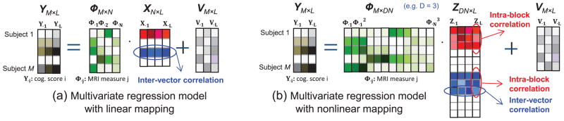
Illustration of (a) multivariate regression model with linear mapping and (b) multivariate regression model with nonlinear mapping.

In our prior work [10], we modeled two specific structures in X. One was the row-sparse structure (i.e., X had only a few nonzero rows), since the brain circuitry relevant to a certain cognition task typically involves a small number of imaging markers, and these markers more or less affect all the cognitive scores under the task. The second was the correlation among entries of the same nonzero block in X. Jointly exploiting the two structures, our previous algorithm [10] achieved better performance than state-of-the-art algorithms which only exploited row-sparse structure.

However, one possible limitation in this model is that a subject’s cognitive score under a task is modeled as a linear function of his/her MRI measures. For example, for the m-th subject, the cognitive score under the l-th task is modeled as

$$Y_{m,l}={\mathrm{\Phi }}_{m,1}{X}_{1,l}+{\mathrm{\Phi }}_{m,2}{X}_{2,l}+\cdots +{\mathrm{\Phi }}_{m,N}{X}_{N,l}+V_{m,l}.$$

A linear model might have limited flexibility in capturing the complex relationship between Y_m,l and Φ_m,n(∀n).

A more powerful model is to consider a nonlinear relationship between Y_m,l and Φ_m,n(∀n). To achieve this, we use polynomials to model the nonlinear relationship:

$$Y_{m,l}={\mathrm{\Phi }}_{m,1}{Z}_{1,l}+{\mathrm{\Phi }}_{m,1}^2{Z}_{2,l}+\cdots +{\mathrm{\Phi }}_{m,1}^{d_1}{Z}_{d_1,l}+\cdots +{\mathrm{\Phi }}_{m,N}{Z}_{c+1,l}+{\mathrm{\Phi }}_{m,N}^2{Z}_{c+2,l}+\cdots +{\mathrm{\Phi }}_{m,N}^{d_g}{Z}_{c+d_g,l}+V_{m,l}$$ (21)

where $c={\sum }_{i=1}^{g-1}{d}_i$. Note that if the MRI measure Φ_m,1 has influence on the subject’s cognitive scores, the associated coefficients Z_1,l, Z_2,l, ···, Z_d1l tend to be nonzero together (but with different amplitudes), and thus Z_1,l, Z_2,l, ···, Z_d1l are correlated. This correlation is in fact the intra-block correlation stated before. The same holds for other MRI measures Φ_m,j(j = 2, ···, N). Writing the relation (21) for all m, l, we obtain the following model in matrix form:

$$\begin{array}{l}\mathbf{Y}\triangleq \left[\begin{array}{ccc}{Y}_{1,1}& \cdots & Y_{1,L}\\ Y_{2,1}& \cdots & Y_{2,L}\\ ⋮& \cdots & ⋮\\ Y_{M,1}& \cdots & Y_{M,L}\end{array}\right]\\ =\left[\begin{array}{cccccc}{\mathrm{\Phi }}_{1,1}& \cdots & {\mathrm{\Phi }}_{1,1}^{d_1}& \cdots & {\mathrm{\Phi }}_{1,N}^{d_g-1}& {\mathrm{\Phi }}_{1,N}^{d_g}\\ {\mathrm{\Phi }}_{2,1}& \cdots & {\mathrm{\Phi }}_{2,1}^{d_1}& \cdots & {\mathrm{\Phi }}_{2,N}^{d_g-1}& {\mathrm{\Phi }}_{2,N}^{d_g}\\ ⋮& ⋮& ⋮& \cdots & ⋮& ⋮\\ {\mathrm{\Phi }}_{M,1}& \cdots & {\mathrm{\Phi }}_{M,1}^{d_1}& \cdots & {\mathrm{\Phi }}_{M,N}^{d_g-1}& {\mathrm{\Phi }}_{M,N}^{d_g}\end{array}\right]·\left[\begin{array}{ccc}{Z}_{1,1}& \cdots & Z_{1,L}\\ ⋮& \cdots & ⋮\\ Z_{d_1,1}& \cdots & Z_{d_1,L}\\ ⋮& \cdots & ⋮\\ Z_{c+d_g-1,1}& \cdots & Z_{c+d_g-1,L}\\ Z_{c+d_g,1}& \cdots & Z_{c+d_g,L}\end{array}\right]+\mathbf{V}\end{array}$$ (22)

$$\triangleq \mathbf{\Psi }\mathbf{Z}+\mathbf{V}.$$ (23)

Note that the matrix Z has the block structure as in (2), and has both the intra-block correlation and the inter-vector correlation (which is inherited from the model (20)). Therefore, the model (23) is exactly the model (1) under the assumption (2), and thus our proposed algorithm can be directly used.

Since our proposed algorithm exploits both the inter-vector and intra-block correlations and can be used to model the nonlinear relationship between predictors and responses, we name it CORNLIN (CORrelation- and NonLINearity-aware SBL). Note that, in this work, all tasks (i.e., predicting multiple cognitive scores) are coupled via inter-vector correlations and all polynomials are coupled via intra-block correlations. Below, we report our experimental results using the third-order polynomial function in (23), i.e., d₁ = d₂ = ··· = d_g = 3 (See Fig. 1(b) for the illustration of the model). These results are among the best through nested cross-validation for tuning the polynomial order parameter. Besides, as in many studies [16], each column of X and Y is normalized to have zero mean and unit standard deviation.

VI. Experimental Results

A. Datasets

The proposed algorithm, CORNLIN, was empirically evaluated using the MRI and cognitive data obtained from the Alzheimer’s Disease Neuroimaging Initiative (ADNI) database (adni.loni.usc.edu). One goal of ADNI has been to test whether serial MRI, positron emission tomography (PET), other biological markers, and clinical and neuropsychological assessment can be combined to measure the progression of mild cognitive impairment (MCI) and early AD. For up-to-date information, see www.adni-info.org.

In our experiments, 222 healthy control (HC) participants and 171 patients with AD were included. Their characteristics are summarized in Table I. Baseline MRI scan of each subject was acquired on 1.5T GE, Philips, and Siemens MRI scanners using a magnetization prepared rapid acquisition gradient echo (MP-RAGE) sequence that was selected and tested by the MRI Core of the ADNI consortium [30]. Further details regarding the scan protocol can be found in [31] and at www.adni-info.org. The FreeSurfer V4 software was used to process the baseline structural MRI scan of each subject, and to extract thickness measures of 34 cortical regions of interests (ROIs) and volume measures of 15 cortical and subcortical regions of interest (ROIs) from each hemisphere (totally 98 imaging measures) [32], [33]. Four sets of cognitive scores [34] were examined (Table II): Alzheimer’s Disease Assessment Scale (ADAS), Mini-Mental State Exam (MMSE), Rey Auditory Verbal Learning Test (RAVLT), and Trail Making Test (TRAILS). ADAS is a global measure incorporating the core syptoms of AD [35]. MMSE examines orientation to time and place, attention and calculation, immediate and delayed recall of words, language and visuo-constructional functions [36]. RAVLT is a measure of verbal memory which consists of eight recall trials and a recognition test [37]. TRAILS, a neuropsychological test of visual attention and task switching, consists of two parts in which the subject is instructed to connect a set of 25 dots as fast as possible while still maintaining accuracy [38], [39]. Details about these neuropsychological tests are available in the ADNI procedure manuals (www.adni-info.org). All the baseline cognitive scores were pre-adjusted for removing the effects of four covariates (the baseline age, gender, education, and handedness) and all the MRI measures were pre-adjusted for the same four covariates plus total intracranial volume (ICV).

TABLE I.

Participant characteristics.

Category	HC	AD	p-value
Gender (M/F)	114/108	86/85	0.835
Handedness (R/L)	205/17	161/10	0.482
Baseline Age (years)	75.93 ± 5.08	75.67 ± 7.36	0.680
Education (years)	15.97 ± 2.84	14.74 ± 3.08	< 0.001

TABLE II.

Description of the cognitive scores.

Score Name		Description
ADAS		Alzheimer’s Disease Assessment Scale
MMSE		Mini-Mental State Exam score
RAVLT	TOTAL T30 RECOG	Total score of the first 5 learning trials 30 minute delay total number of words recalled 30 minute delay recognition score
TRAILS	TRAILSA TRAILSB TR(B-A)	Trail Making test A score Trail Making test B score TRAILSB-TRAILSA

B. Comparison with Competing Methods

To show the superior performance of CORNLIN, five state-of-the-art or classical algorithms were used for comparison. Each algorithm is a representative of a different group of algorithms. They are the T-MSBL-FP algorithm [10], the mixed ℓ₂/ℓ₁ minimization algorithm [40], the multi-task compressive sensing algorithm (MT-CS) [41], the Elastic Net algorithm [42], and the ridge regression [43]. T-MSBL-FP is a fast variant of T-MSBL algorithm [20], which is a sparse Bayesian learning algorithm exploiting inter-vector correlation among the regression coefficients. Mixed ℓ₂/ℓ₁ is a representative of convex algorithms based on multivariate regression model. Both T-MSBL-FP and Mixed ℓ₂/ℓ₁ exploit the row sparsity of the coefficient matrix. MT-CS is a Bayesian multi-task learning algorithm. Elastic Net adopts a penalty function which is a convex combination of the ℓ₁ lasso and ℓ₂ ridge. Ridge is a special case of Elastic Net by dropping the ℓ₁ constraint. In our experiments, the parameters of these algorithms were automatically tuned by nested cross-validation.

All the algorithms were applied to predict the cognitive scores using the MRI measures. For MRI measures, we had thickness or volume measures of 49 ROIs from each hemisphere. Then the bilateral measures were averaged to generate one single measure for each ROI. For cognitive scores, we used all four sets of baseline cognitive scores (ADAS, MMSE, RAVLT and TRAILS). As in [6], [10], [11], the Pearson’s correlation coefficient r between the actual and predicted cognitive scores was computed to measure the prediction performance for each set of cognitive scores (i.e., ADAS, MMSE, RAVLT, and TRAILS). For each set of scores, five-fold cross-validation was used to obtain the mean of r and its standard error of mean (SEM). We also tested the explained variance by the regression model as a performance criterion and it yielded similar results.

In the first set of experiments, we compared CORNLIN (a nonlinear model) with five competing methods (all linear models). Shown in Fig. 2 and Table. III (see only linear columns for competing methods) is the cross validation prediction performance; and shown in Fig. 3 are example scatter plots of actual and predicted scores. CORNLIN outperformed all the competing algorithms for almost all sets of scores except that the Elastic Net achieved better performance than CORNLIN in predicting TOTAL score. To examine whether these improved prediction performances were significant, we randomly created 50 5-fold data partitions and compared the corresponding cross-validation performances measured by the mean correlation coefficient between predicted and actual scores using a pairwise t-test. CORNLIN significantly outperformed other methods in almost all the cases (p ≤ 2.76×10⁻⁵) except: (1) Elastic Net significantly outperforming CORNLIN for predicting TOTAL (p = 1.51×10⁻⁵) and (2) no significant difference between CORNLIN and Mixed ℓ₂/ℓ₁ for predicting TOTAL (p = 0.721). In particular, comparing CORNLIN to T-MSBL-FP, we can see the improved performance. Since the linear model used by T-MSBL-FP is a special case of the nonlinear model used by CORNLIN when d₁ = · · · = d_g = 1, these results show that the nonlinear model with the ability to exploit the intra-block correlation can better capture the relation between the predictors (the MRI measures) and the responses (the cognitive scores) than the linear model.

Fig. 2.

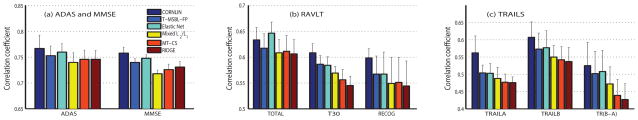
Comparison of prediction performances measured by mean of correlation coefficients and its standard error of mean (SEM) among six algorithms.

TABLE III.

Prediction performances measured by mean correlation coefficients.

	CORNLIN	T-MSBL-FP		Elastic net		Mixed ℓ2/ℓ1		MT-CS		Ridge
Test cases	Nonlinear	Linear	Nonlinear	Linear	Nonlinear	Linear	Nonlinear	Linear	Nonlinear	Linear	Nonlinear
ADAS	0.767	0.753	0.764	0.760	0.762	0.740	0.711	0.746	0.735	0.746	0.738
MMSE	0.758	0.740	0.742	0.748	0.746	0.718	0.626	0.726	0.694	0.731	0.723
TOTAL	0.633	0.617	0.620	0.646	0.648	0.608	0.520	0.611	0.602	0.606	0.586
T30	0.608	0.586	0.586	0.584	0.581	0.569	0.494	0.556	0.528	0.545	0.483
RECOG	0.598	0.567	0.568	0.567	0.572	0.549	0.563	0.551	0.545	0.544	0.558
TRAILSA	0.562	0.504	0.522	0.503	0.509	0.488	0.403	0.477	0.512	0.476	0.515
TRAILSB	0.607	0.573	0.587	0.577	0.572	0.550	0.461	0.542	0.5022	0.537	0.516
TR(B-A)	0.525	0.502	0.514	0.508	0.502	0.472	0.383	0.439	0.387	0.427	0.381

Fig. 3.

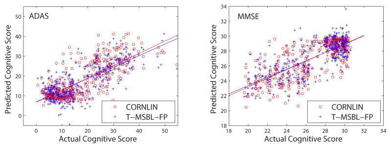
Example scatter plots of actual and predicted cognitive scores.

Fig. 4 shows that the heat maps of the regression coefficients calculated by CORNLIN, T-MSBL-FP, and Elastic Net for all the cognitive tasks in the four sets. Every five columns form a column block (sketched by black vertical lines) to represent the regression coefficients in the five-fold cross validation. In Fig. 4(b–c), each row corresponds to an MRI measure which is an average of left and right measures, and each column block corresponds to a cognitive task. In Fig. 4(a), since we adopted the nonlinear model using the third-order polynomial, every three column blocks (e.g., ADAS¹, ADAS², ADAS³) correspond to a cognitive task, representing the regression coefficients for the 1st, 2nd, and 3rd orders of the polynomial, respectively. In addition, the blue color indicates negative correlation while the red indicates positive correlation and the green indicates zero correlation. The larger the absolute value of a coefficient is, the more important its corresponding MRI measure is in predicting the corresponding cognitive score.

Fig. 4.

Heat maps of regression coefficients of five-fold cross-validation trials for (a) CORNLIN, (b) T-MSBL-FP, and (c) the Elastic Net. Results for volume measures are shown in top 15 rows, and those for thickness measures in bottom 34 rows. Detailed descriptions are given in the text.

The pattern obtained by CORNLIN is sparser than those obtained by T-MSBL-FP, the Elastic Net and other compared algorithms (not shown due to space constraints), making the results easier to interpret. The imaging biomarkers identified by CORNLIN yielded promising patterns (Fig. 4) that are expected from prior knowledge on neuroimaging and cognition. The tasks in ADAS and MMSE aimed to reflect overall cognitive impairment, while the result of CORNLIN showed important AD-relevant imaging biomarkers such as hippocampal volume (HippVol), amygdala volume (AmygVol), and entorhinal cortex thickness (EntCtx). The tasks in RAVLT (i.e., TOTAL, T30 and RECOG) aimed to test verbal learning memory, while the result of CORNLIN highlighted regions relevant to learning and memory, such as hippocampus (HippVol) and entorhinal cortex (EntCtx). The tasks in TRAILS (i.e., TRAILSA, TRAILSB, TR(B-A)) aimed to test a combination of visual, motor and executive functions, while the result of CORNLIN showed regions in temporal lobe (EntCtx), parietal lobe (InfParietal), and ventricle (InfLatVent).

All the above results demonstrated that the proposed CORN-LIN algorithm not only yielded higher prediction accuracy, but also had a desired ability to discover a small set of imaging biomarkers that were easier to interpret and were consistent with prior findings (e.g., [44]–[46]). The algorithm could provide important information for understanding brain structural changes related to cognitive status, and could potentially help characterize the progression of AD.

C. Comparison with Nonlinear Competing Methods

In previous experiments, the competing algorithms were carried out using their original linear form (20). In the second set of experiments, we expanded the competing algorithms using the nonlinear paradigm shown in (23) in order to see the benefits of the block structure and exploiting the intra-block correlation in our model. We used the 3rd order polynomials to construct the predictor matrix, Φ. Note that the five competing algorithms just used a nonlinear predictor matrix without any block structure. The nonlinear columns in Table III show the comparison of prediction performances. We can still see that CORNLIN outperformed the nonlinear extensions of other algorithms in most cases. We also calculated the p-value of mean correlation coefficients between CORNLIN and the competing algorithms as what we did in Section VI-B. CORNLIN significantly outperformed the nonlinear versions of the competing methods in almost all the cases (p ≤ 1.89 × 10⁻³) except: (1) Elastic Net significantly outperformed CORNLIN for predicting TOTAL (p = 7.31 × 10⁻¹²) and (2) no significant difference between CORNLIN and Elastic Net for predicting ADAS (p=0.354). In particular, the only difference between CORNLIN and nonlinear T-MSBL-FP was that CORNLIN exploited the intra-block correlation while nonlinear T-MSBL-FP did not. This demonstrated that exploiting intra-block correlation could further improve the prediction performance of a nonlinear model.

D. Comparison in Different Orders of Polynomials

In the above experiment, the third-order polynomial was used in the nonlinear model. However, we may adopt any order of polynomials. To better understand the relationship between different polynomial orders and prediction performance, we carried out experiments on the four sets of cognitive scores using polynomials from the 1st order to the 6th order (Fig. 5). The 3rd order polynomial achieved the highest prediction accuracy in predicting MMSE and RAVLT, while the 4th order polynomial had the best prediction performance for TRAILS and ADAS. From Fig. 5, we can see that adopting the order of polynomial up to 4th is a good choice for predicting all the four sets of cognitive scores, considering the prediction performance and model complexity.

Fig. 5.

Prediction performances using polynomials of different orders.

E. Comparison using Different Types of Imaging Measures

In this section, we report the performance comparison result on using three types of MRI measures to predict cognitive scores with CORNLIN. As described in Section VI-A, for each participant there are totally 98 MRI measures (thickness or volume measures) extracted from 49 cortical/subcortical ROIs in each hemisphere. For simplicity, we can average bilateral measures to generate one single measure for each ROI and thus obtain 49 averaged MRI measures for each participant. We call such measures the LR-Average measures. So far all the experiments reported above employed this kind of imaging measures as predictors.

Since two hemispheres may contribute to different cognitive functions, sometimes it is better to look at the ROIs in left and right hemisphere separately. Thus, we performed another experiment by employing all 98 MRI measures from both hemispheres for each participant and treating each MRI measure separately. For example, in linear model (20), Φ_1,1 is the MRI measure of the 1st ROI in the left hemisphere of Subject 1, and Φ_1,2 is the MRI measure of the 1st ROI in the right hemisphere of this subject. We call these measures the LR-Separate measures, which is our second type of MRI measures. Fig. 6(a) shows how to construct the Φ matrix in a nonlinear model using LR-Separate measures.

Fig. 6.

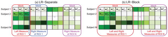
Illustration of constructing Φ matrix in nonlinear model using (a) LR-Separate and (b) LR-Block, respectively.

Given that most ROIs have a bilaterally symmetric pattern in terms of their volumetric or thickness measures, it is reasonable to hypothesize that the regression coefficients of the left and right sides of the same ROI are correlated and this relationship should be embraced. Thus, another choice is to bundle each pair of left and right ROIs together so that bilateral biomarkers can be identified together. Accordingly, in our third type of MRI measures, which is denoted by LR-Block, the left and right measures from corresponding ROIs and their associated terms of polynomials are concatenated to form a column block in Φ matrix (as shown in Fig. 6(b)). If LR-Block and third-order polynomial are adopted, the coefficient matrix Z has block size of 6 (i.e, d_i = 6, ∀i).

For comparison, CORNLIN was applied to a nonlinear regression model with third-order polynomials for predicting the four sets of cognitive scores (ADAS, MMSE, RAVLT, and TRAILS) from the three kinds of MRI measures (LR-Average, LR-Separate, and LR-Block), respectively. Five-fold cross-validation was adopted to evaluate the robustness of each kind of MRI measures. Table IV shows the performance comparison measured by mean and standard error of mean (SEM) of correlation coefficients between actual and predicted scores. Average measures (LR-Average) performed better than individual measures (LR-Separate and LR-Block) for MMSE and TRAILS, while the individual ones did better than average ones for ADAS ad RAVLT. The performances of LR-Separate and LR-Block were similar: LR-Separate performed slightly better for ADAS and RAVLT, while LR-Block did slightly better for MMSE and TRAILS.

TABLE IV.

Prediction performances (mean±sem of correlation coefficients) using three MRI measures models in CORNLIN

Test cases	LR-Average	LR-Separate	LR-Block
ADAS	0.767 ± 0.026	0.768 ± 0.020	0.766 ± 0.017
MMSE	0.758 ± 0.011	0.745 ± 0.010	0.749 ± 0.009
TOTAL	0.633 ± 0.024	0.660 ± 0.015	0.649 ± 0.016
T30	0.608 ± 0.018	0.626 ± 0.008	0.625 ± 0.005
RECOG	0.598 ± 0.018	0.566 ± 0.022	0.565 ± 0.028
TRAILSA	0.562 ± 0.050	0.534 ± 0.067	0.551 ± 0.055
TRAILSB	0.607 ± 0.044	0.572 ± 0.039	0.586 ± 0.045
TR(B-A)	0.525 ± 0.067	0.491 ± 0.056	0.499 ± 0.069

Fig. 7 shows the heat maps of regression coefficients in five-fold cross-validation trials for predicting RAVLT cognitive scores using LR-Separate and LR-Block MRI measures. The arrangement of the heap maps in Fig. 7 is almost as same as those in Fig. 4, except that in Fig. 7 every two column blocks for each cognitive score variable correspond to the ROIs in the left and right hemispheres while in Fig. 4 every column block for each cognitive score variable corresponds to the averaged MRI measures (LR-Average) used. From Fig. 7, we can see that the biomarkers identified by LR-Block are more consistent than those detected by LR-Separate in the five-fold cross-validation trials. In addition, there are more bilateral regions identified by LR-Block than those identified by LR-Separate (See HippoVol region in both heat maps). Fig. 8 shows visualization of the regression coefficients for RAVLT-TOTAL mapped onto the brain. LR-Block demonstrated a more symmetric pattern than LR-Separate. For highly correlated features (e.g., left and right measures in our case), we do not expect the block design to yield significantly enhanced prediction accuracy based on two observations: (1) these features possess almost identical information, (2) it is sufficient to select just one feature (e.g., by flat sparsity strategy like Lasso) to represent the entire feature group and achieve similar prediction performance. However, as shown in Fig. 7 and Fig. 8, the block design has the potential to select all the features in each relevant block and yield more stable and biologically more meaningful results.

Fig. 7.

Heat maps of 5-fold cross-validation regression coefficients in CORNLIN for predicting RAVLT scores using (a) LR-Separate and (b) LR-Block.

Fig. 8.

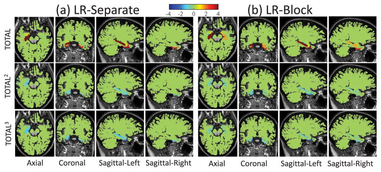
Brain maps of the average regression coefficients of five-fold cross-validation trials when using (a) LR-Separate and (b) LR-Block measures to predict cognitive score RAVLT-TOTAL with a third-order polynomial model.

VII. Discussion

Our proposed CORNLIN algorithm exploits not only inter-vector correlation among coefficient vectors, but also intra-block correlation in each coefficient vector, which provides feasibility to model nonlinear relation between the responses and the predictors. Compared to our prior method [10], T-MSBL-FP, which only uses inter-vector correlation, CORN-LIN has improved prediction performance for all four sets of cognitive scores (See Fig. 2). This demonstrates that using the nonlinear model coupled with the block design has the potential to better capture the complex relationship between brain structure and cognitive decline. In this study, we used polynomials to represent a nonlinear relationship. Note that the polynomial model can also detect linear patterns, since the latter is a special case of the former. Investigating powerful nonlinear functions (e.g., polynomial or exponential) to capture the complicated nonlinear relationships and their biological interpretation is an interesting future direction.

CORNLIN can adaptively estimate and exploit the inter-vector correlation and intra-block correlation in regression coefficients matrix. As described in Section III, inter-vector correlation is modeled by an unknown positive definite matrix B and intra-block correlation is captured by unknown positive definite matrices A_i. The parameter γ_i is an unknown nonnegative scalar determining zero or non-zero property of a block and thus controlling the sparsity of selected features. The parameter λ is an unknown regularizer. All the parameters can be automatically tuned using our effective learning rules. This relaxes the efforts of users to choose suitable values for the parameters in the training phase. What’s more, other than performing feature selection in a separate preprocessing step [12], [47], [48], CORNLIN automatically determines relevant imaging features and uses them to make prediction in one consistent modeling framework. Although A_i and B can be automatically tuned, CORNLIN also provides options for the users to input their own A_i or B for modeling the correlations. Such prior/expert knowledge may provide more efficient solutions for prediction. This setting makes CORNLIN more flexible to use. Interesting future directions could be to study how to construct A_i and B and how to develop more efficient algorithms with better performance.

In this study, imaging measures are important inputs (predictors) to our multivariate regression model. From Section VI-E, we can see that different uses of imaging measures may achieve different prediction accuracies or identify different biomarkers. Exploring the inner structure or relationship among predictors is an interesting topic. This study provides one way to manipulate the predictors by using block structure. We can not only extend linear mapping to nonlinear mapping by placing the terms of a polynomial model into one block, but also bundle related imaging measures into one block, as what we did for LR-Block. Using block structures, users can easily incorporate biologically meaningful structures or knowledge-guided brain circuitries into the regression model and then apply CORNLIN to solve it. There are other correlations which can be exploited to improve performance, such as correlation among brain regions or temporal correlation among longitudinal measures. These are more challenging tasks and require more complicated models and algorithms, which is an interesting future direction to explore.

Compared to existing sparse regression algorithms [8], [9], [13], [20], [21], [49], CORNLIN is the first one to exploit and explicitly estimate both the intra-block and inter-vector correlations in regression coefficient matrices. In [8], the most basic sparse Bayesian learning algorithm was used, and no structures were exploited but sparsity of regression coefficients. In [9] the coefficient matrix X (denoted by W in [9]) was penalized by using a combination of ℓ_2,1 norm and ℓ₁ norm of X, where the ℓ_2,1 norm enforced the row-sparsity of X and the ℓ₁ norm enforced the entry-wise sparsity of X. The intra-block correlation and the inter-vector correlation in X were not estimated. Some prior studies exploited smoothness among regression coefficients by using a Laplacian matrix [13] or a kind of fused Lasso penalties [50]. However, smoothness is a special kind of correlation structures. It is not helpful when adjacent regression coefficients are not smooth (but still correlated), as shown in [20] in the comparison between the T-MSBL algorithm [20] and a smoothness constrained sparse algorithm in [51]. More general correlation structures were studied in [10], [20], [21], which did not constrain the smoothness in regression coefficients. However, in [10], [20], the algorithms only exploited the inter-vector correlation in the coefficient matrices. In [21], only the intra-block correlation in coefficient vectors was exploited. It is the first time that the two kinds of correlation are jointly exploited in our algorithm.

In this work, we empirically evaluated the proposed algorithm in an application where we had more samples than features. An interesting future topic is to conduct performance comparison between the proposed method and the competing methods in a high dimensional setting such as using detailed voxel-based image measures as features, where the number of features is greater than the number of samples.

VIII. Conclusion

Based on a sparse multivariate regression model, this paper proposed a sparse Bayesian learning algorithm, which not only exploited the inter-vector correlation in the regression coefficient matrix, but also considered the intra-block correlation in each coefficient vector. In addition, the algorithm offered a flexible scheme to examine the nonlinear relationship between the responses and the predictors. We illustrated its superiority by applying it to the prediction of cognitive scores of subjects from their MRI measures. The prediction performance of different orders of polynomials was discussed, as well as the comparison of three types of MRI measures. Compared to state-of-the-art algorithms, the proposed algorithm not only showed the highest prediction accuracy, but also demonstrated the ability to accurately identify imaging biomarkers that are consistent with prior knowledge.

Appendix

A. Learning Rule for γ_i

To derive the learning rule for γ_i, we use a bound-optimization method [21], since the learning rule based on this method has a good balance between estimation accuracy and speed.

Note that the first term in the cost function (12) is convex with respect to γ, and the second term in the cost function is concave with respect to γ. Since the goal is to minimize the cost function, we consider an upper-bound for the second term, and then minimize the upper-bound of the cost function.

An upper-bound for the second term is its supporting hyperplane. Let γ* be a given point in the γ-space. We have

$$log\mid {\mathbf{\sum }}_{\mathbf{y}}\mid \le \sum _{i=1}^g\text{Tr}({({\mathbf{\sum }}_{\mathbf{y}}^{\ast })}^{-1}{\mathbf{D}}_{·[i]}({\mathbf{A}}_i\otimes \mathbf{B}){\mathbf{D}}_{·[i]}^T)({\gamma }_i-{\gamma }_i^{\ast })+log\mid {\mathbf{\sum }}_{\mathbf{y}}^{\ast }\mid$$ (24)

where ${\mathbf{\sum }}_{\mathbf{y}}^{\ast }={\mathbf{\sum }}_{\mathbf{y}}{\mid }_{\mathit{\gamma }={\mathit{\gamma }}^{\ast }}$, and D_·[i] = Φ_·[i] ⊗ I_L, and Φ_·[i] is the i-th block of Φ corresponding to X_[i]·. Besides, note that:

$$\begin{array}{l}{\mathbf{y}}^T{(\lambda \mathbf{I}\otimes \mathbf{B}+\mathbf{D}(\mathbf{\Pi }\otimes \mathbf{B}){\mathbf{D}}^T)}^{-1}\mathbf{y}\\ \stackrel{(\ast )}{=}{\lambda }^{-1}{\mathbf{y}}^T\left\{\mathbf{I}\otimes {\mathbf{B}}^{-1}-(\mathbf{I}\otimes {\mathbf{B}}^{-1})\mathbf{D}·{[{\lambda }^{-1}{\mathbf{D}}^T(\mathbf{I}\otimes {\mathbf{B}}^{-1})\mathbf{D}+{\mathbf{\Pi }}^{-1}\otimes {\mathbf{B}}^{-1}]}^{-1}·{\mathbf{D}}^T(\mathbf{I}\otimes {\mathbf{B}}^{-1}){\lambda }^{-1}\right\}\mathbf{y}\\ \stackrel{(\ast \ast )}{=}{\lambda }^{-1}{\mathbf{y}}^T(\mathbf{I}\otimes {\mathbf{B}}^{-1})(\mathbf{y}-\mathbf{D}\mathit{\mu })\\ ={(\mathbf{y}-\mathbf{D}\mathit{\mu })}^T{(\lambda \mathbf{I}\otimes \mathbf{B})}^{-1}(\mathbf{y}-\mathbf{D}\mathit{\mu })+{\mathit{\mu }}^T{\mathbf{D}}^T{(\lambda \mathbf{I}\otimes \mathbf{B})}^{-1}\mathbf{y}-{\mathit{\mu }}^T{\mathbf{D}}^T{(\lambda \mathbf{I}\otimes \mathbf{B})}^{-1}\mathbf{D}\mathit{\mu }\\ \stackrel{(\ast \ast \ast )}{=}{(\mathbf{y}-\mathbf{D}\mathit{\mu })}^T{(\lambda \mathbf{I}\otimes \mathbf{B})}^{-1}(\mathbf{y}-\mathbf{D}\mathit{\mu })+{\mathit{\mu }}^T({\mathbf{\sum }}^{-1}-{\mathbf{D}}^T{(\lambda \mathbf{I}\otimes \mathbf{B})}^{-1}\mathbf{D})\mathit{\mu }\\ \stackrel{(\ast \ast \ast \ast )}{=}{(\mathbf{y}-\mathbf{D}\mathit{\mu })}^T{(\lambda \mathbf{I}\otimes \mathbf{B})}^{-1}(\mathbf{y}-\mathbf{D}\mathit{\mu })+{\mathit{\mu }}^T{(\mathbf{\Pi }\otimes \mathbf{B})}^{-1}\mathit{\mu }\end{array}$$ (25)

where (*) used the Matrix Inversion Lemma, (**) used (9) and (8), (***) used (9), and (****) used (8).

Substituting (24) and (25) into the cost function (12), we obtain the upper bound:

$$\mathcal{G}({\{{\gamma }_i\}}_i)=\frac{1}{\lambda }{(\mathbf{y}-\mathbf{D}\mathit{\mu })}^T{(\mathbf{I}\otimes \mathbf{B})}^{-1}(\mathbf{y}-\mathbf{D}\mathit{\mu })+\sum _{i=1}^g\text{Tr(}{({\mathbf{\sum }}_{\mathbf{y}}^{\ast })}^{-1}{\mathbf{D}}_{·[i]}({\mathbf{A}}_i\otimes \mathbf{B}){\mathbf{D}}_{·[i]}^T)({\gamma }_i-{\gamma }_i^{\ast })+{\mathit{\mu }}^T{(\mathbf{\Pi }\otimes \mathbf{B})}^{-1}\mathit{\mu }+log\mid {\mathbf{\sum }}_{\mathbf{y}}^{\ast }\mid .$$ (26)

Taking the derivative of ({γ_i}_i) with respect to γ_i, we finally obtain the following learning rule

$${\gamma }_i\leftarrow \sqrt{\frac{{\mathit{\mu }}_{[i]}^T({\mathbf{A}}_i^{-1}\otimes {\mathbf{B}}^{-1}){\mathit{\mu }}_{[i]}}{\text{Tr}({({\mathbf{\sum }}_{\mathbf{y}})}^{-1}{\mathbf{D}}_{·[i]}({\mathbf{A}}_i\otimes \mathbf{B}){\mathbf{D}}_{·[i]}^T)}}$$ (27)

where μ_[i] ∈ ℝ^d_iL×1, and the quantity ${\mathbf{\sum }}_{\mathbf{y}}^{\ast }$ in (26) is replaced with Σ_y, keeping in mind that Σ_y is calculated using the estimated parameters in the previous iteration. Note that the rule (27) can be rewritten as

$${\gamma }_i\leftarrow \sqrt{\frac{L^{-1}\text{Tr}({\mathbf{X}}_{[i]·}{\mathbf{B}}^{-1}{\mathbf{X}}_{[i]·}^T{\mathbf{A}}_i^{-1})}{\text{Tr}({(\lambda \mathbf{I}+\mathbf{\Phi }\mathbf{\Pi }{\mathbf{\Phi }}^T)}^{-1}{\mathbf{\Phi }}_{·[i]}{\mathbf{A}}_i{\mathbf{\Phi }}_{·[i]}^T)}}$$ (28)

where X is estimated by (11).

B. Learning Rule for B

Noting that

$$log\mid {\mathbf{\sum }}_{\mathbf{y}}\mid =Llog\mid \lambda \mathbf{I}+\mathbf{\Phi }\mathbf{\Pi }{\mathbf{\Phi }}^T\mid +Mlog\mid \mathbf{B}\mid$$

and the result in (25), we can re-express the cost function (12) as

$$\mathcal{L}(\mathbf{B})=Llog\mid \lambda \mathbf{I}+\mathbf{\Phi }\mathbf{\Pi }{\mathbf{\Phi }}^T\mid +Mlog\mid \mathbf{B}\mid +{(\mathbf{y}-\mathbf{D}\mathit{\mu })}^T{(\lambda \mathbf{I}\otimes \mathbf{B})}^{-1}(\mathbf{y}-\mathbf{D}\mathit{\mu })+{\mathit{\mu }}^T{(\mathbf{\Pi }\otimes \mathbf{B})}^{-1}\mathit{\mu }.$$ (29)

Setting the derivative to zero, we obtain

$${\mathbf{B}}^{+}\leftarrow \sum _{i=1}^g\frac{{\mathbf{X}}_{[i]·}^T{\mathbf{A}}_i^{-1}{\mathbf{X}}_{[i]·}}{{\gamma }_i}+\frac{{(\mathbf{Y}-\mathbf{\Phi }\mathbf{X})}^T(\mathbf{Y}-\mathbf{\Phi }\mathbf{X})}{\lambda }$$ (30)

$$\mathbf{B}\leftarrow {\mathbf{B}}^{+}/{\Vert {\mathbf{B}}^{+}\Vert }_{\mathcal{F}}$$ (31)

where the goal of (31) is to avoid the ambiguity among A_i, γ_i and B. In (30) the first term is data-related, while the second term is noise-related.

C. Learning Rule for A_i

From the original cost function (12) or the equivalent one (29), one can derive a learning rule for A_i(∀i), but it costs large computational load due to the coupling between A_i(∀i) and B. If assuming L ≥ max{d₁, …, d_g}, one can derive a learning rule with light computational load, but this condition narrows applications. For example, in our applications this condition does not necessarily hold. Fortunately, by decomposing our original model into two coupling sub-models, we can derive an efficient learning rule for A_i(∀i) (and other parameters).

Assume B has been estimated. Letting $\stackrel{\sim }{\mathbf{Y}}\triangleq {\mathbf{YB}}^{-\frac{1}{2}},\stackrel{\sim }{\mathbf{X}}\triangleq {\mathbf{XB}}^{-\frac{1}{2}}$, and $\stackrel{\sim }{\mathbf{V}}\triangleq {\mathbf{VB}}^{-\frac{1}{2}}$, the original model (1) becomes

$$\stackrel{\sim }{\mathbf{Y}}=\mathbf{\Phi }\stackrel{\sim }{\mathbf{X}}+\stackrel{\sim }{\mathbf{V}},$$ (32)

where the columns of X̃ are independent, and so does Ṽ. Now the model is a block sparse Bayesian learning model [21] with multiple measurement vectors.

Following the EM method in [20], [21], we can easily derive the learning rule for A_i(∀i):

$${\mathbf{A}}_i\leftarrow \frac{1}{L}\sum _{l=1}^L\frac{{\mathbf{\sum }^{\mathbf{\sim }}}_{[i]}+{\stackrel{\sim }{\mathit{\mu }}}_{[i]l}{\stackrel{\sim }{\mathit{\mu }}}_{[i]l}^T}{{\gamma }_i},$$ (33)

where

$$\begin{array}{l}\mathbf{\sum }^{\mathbf{\sim }}=\mathbf{\Pi }-\mathbf{\Pi }{\mathbf{\Phi }}^T{(\lambda \mathbf{I}+\mathbf{\Phi }\mathbf{\Pi }{\mathbf{\Phi }}^T)}^{-1}\mathbf{\Phi }\mathbf{\Pi }\\ \stackrel{\sim }{\mathit{\mu }}=\mathbf{\Pi }{\mathbf{\Phi }}^T{(\lambda \mathbf{I}+\mathbf{\Phi }\mathbf{\Pi }{\mathbf{\Phi }}^T)}^{-1}{\mathbf{YB}}^{-\frac{1}{2}}.\end{array}$$

D. Learning Rule for λ

From the equivalent model (32) and following the EM method in [21], the learning rule for λ can be also derived as follows,

$$\lambda \leftarrow \frac{1}{ML}{\Vert \stackrel{\sim }{\mathbf{Y}}-\mathbf{\Phi }\stackrel{\sim }{\mathit{\mu }}\Vert }_{\mathcal{F}}^2+\frac{1}{M}\text{Tr}(\mathbf{\sum }^{\mathbf{\sim }}{\mathbf{\Phi }}^T\mathbf{\Phi }).$$ (34)

Similar as in [21], at low SNR cases the above learning rule should be modified to

$$\lambda \leftarrow \frac{1}{ML}{\Vert \stackrel{\sim }{\mathbf{Y}}-\mathbf{\Phi }\stackrel{\sim }{\mathit{\mu }}\Vert }_{\mathcal{F}}^2+\frac{1}{M}\sum _{i=1}^g\text{Tr}({\mathbf{\sum }^{\mathbf{\sim }}}_{[i]}{\mathbf{\Phi }}_{·[i]}^T{\mathbf{\Phi }}_{·[i]}),$$ (35)

where Φ_·[i] denotes the consecutive columns in Φ which correspond to the i-th block in X. In noise-free situations, one can simply fix λ to a very small value such as 10⁻¹⁰ instead of performing this learning rule.

References

- 1.McKhann G, Drachman D, et al. Clinical diagnosis of Alzheimer’s disease: Report of the NINCDS-ADRDA work group under the auspices of department of health and human services task force on Alzheimer’s disease. Neurology. 1984;34(7):939–939. doi: 10.1212/wnl.34.7.939. [DOI] [PubMed] [Google Scholar]
- 2.Klöppel S, Stonnington CM, et al. Automatic classification of MR scans in Alzheimer’s disease. Brain. 2008;131(3):681–689. doi: 10.1093/brain/awm319. [DOI] [PMC free article] [PubMed] [Google Scholar]
- 3.Plant C, Teipel SJ, Oswald A, et al. Automated detection of brain atrophy patterns based on MRI for the prediction of Alzheimer’s disease. Neuroimage. 2010;50(1):162–174. doi: 10.1016/j.neuroimage.2009.11.046. [DOI] [PMC free article] [PubMed] [Google Scholar]
- 4.Radanovic M, Pereira FRS, Stella F, et al. White matter abnormalities associated with Alzheimer’s disease and mild cognitive impairment: a critical review of MRI studies. Expert Review of Neurotherapeutics. 2013;13(5):483–493. doi: 10.1586/ern.13.45. [DOI] [PubMed] [Google Scholar]
- 5.Chincarini A, Bosco P, Gemme G, et al. Alzheimers disease markers from structural MRI and FDG-PET brain images. The European Physical Journal Plus. 2012;127(11):1–16. [Google Scholar]
- 6.Stonnington CM, Chu C, et al. Predicting clinical scores from magnetic resonance scans in Alzheimer’s disease. Neuroimage. 2010;51(4):1405–13. doi: 10.1016/j.neuroimage.2010.03.051. [DOI] [PMC free article] [PubMed] [Google Scholar]
- 7.Wang Y, Fan Y, Bhatt PDC. High-dimensional pattern regression using machine learning: From medical images to continuous clinical variables. Neuroimage. 2010;50(4):1519–35. doi: 10.1016/j.neuroimage.2009.12.092. [DOI] [PMC free article] [PubMed] [Google Scholar]
- 8.Shen L, Qi Y, Kim S, et al. Sparse Bayesian learning for identifying imaging biomarkers in AD prediction. MICCAI. 2010:611–618. doi: 10.1007/978-3-642-15711-0_76. [DOI] [PMC free article] [PubMed] [Google Scholar]
- 9.Wang H, Nie F, Huang H, et al. Sparse multi-task regression and feature selection to identify brain imaging predictors for memory performance. ICCV. 2011:557–562. doi: 10.1109/ICCV.2011.6126288. [DOI] [PMC free article] [PubMed] [Google Scholar]
- 10.Wan J, Zhang Z, Yan J, et al. Sparse Bayesian multi-task learning for predicting cognitive outcomes from neuroimaging measures in Alzheimer’s disease. CVPR. 2012:940–947. [Google Scholar]
- 11.Zhang D, Shen D. Multi-modal multi-task learning for joint prediction of multiple regression and classification variables in Alzheimer’s disease. Neuroimage. 2012;59(2):895–907. doi: 10.1016/j.neuroimage.2011.09.069. [DOI] [PMC free article] [PubMed] [Google Scholar]
- 12.Zhang D, Shen D. Predicting future clinical changes of MCI patients using longitudinal and multimodal biomarkers. PLoS One. 2012;7(3):e33182. doi: 10.1371/journal.pone.0033182. [DOI] [PMC free article] [PubMed] [Google Scholar]
- 13.Sabuncu M, Leemput K ADNI. The relevance voxel machine (RVoxM): A self-tuning Bayesian model for informative image-based prediction. IEEE Transactions on Medical Imaging. 2012;31(12):2290–306. doi: 10.1109/TMI.2012.2216543. [DOI] [PMC free article] [PubMed] [Google Scholar]
- 14.Yuan L, Wang Y, Thompson PM, et al. Multi-source feature learning for joint analysis of incomplete multiple heterogeneous neuroimaging data. NeuroImage. 2012;61(3):622–632. doi: 10.1016/j.neuroimage.2012.03.059. [DOI] [PMC free article] [PubMed] [Google Scholar]
- 15.Ye J, Farnum M, et al. Sparse learning and stability selection for predicting MCI to AD conversion using baseline ADNI data. BMC Neurology. 2012;12:46. doi: 10.1186/1471-2377-12-46. [DOI] [PMC free article] [PubMed] [Google Scholar]
- 16.Bunea F, She Y, Ombao H, et al. Penalized least squares regression methods and applications to neuroimaging. NeuroImage. 2011;55(4):1519–1527. doi: 10.1016/j.neuroimage.2010.12.028. [DOI] [PMC free article] [PubMed] [Google Scholar]
- 17.Silver M, Janousova E, et al. Identification of gene pathways implicated in Alzheimer’s disease using longitudinal imaging phenotypes with sparse regression. Neuroimage. 2012;63:1681–1694. doi: 10.1016/j.neuroimage.2012.08.002. [DOI] [PMC free article] [PubMed] [Google Scholar]
- 18.Vounou M, Janousova E, et al. Sparse reduced-rank regression detects genetic associations with voxel-wise longitudinal phenotypes in alzheimer’s disease. Neuroimage. 2012;60(1):700–16. doi: 10.1016/j.neuroimage.2011.12.029. [DOI] [PMC free article] [PubMed] [Google Scholar]
- 19.Carroll MK, Cecchi GA, Rish I, Garg R, Rao AR. Prediction and interpretation of distributed neural activity with sparse models. NeuroImage. 2009;44(1):112–122. doi: 10.1016/j.neuroimage.2008.08.020. [DOI] [PubMed] [Google Scholar]
- 20.Zhang Z, Rao BD. Sparse signal recovery with temporally correlated source vectors using sparse Bayesian learning. IEEE Journal of Selected Topics in Signal Processing. 2011;5(5):912–926. [Google Scholar]
- 21.Zhang Z, Rao BD. Extension of SBL algorithms for the recovery of block sparse signals with intra-block correlation. IEEE Transactions on Signal Processing. 2013;61(8):2009–2015. [Google Scholar]
- 22.Tipping M. Sparse Bayesian learning and the relevance vector machine. Journal of Machine Learning Research. 2001;1:211–244. [Google Scholar]
- 23.Brown P, Vannucci M, Fearn T. Multivariate Bayesian variable selection and prediction. Journal of the Royal Statistical Society: Series B (Statistical Methodology) 1998;60(3):627–641. [Google Scholar]
- 24.Dension DG, Holmes CC, et al. Bayesian Methods for Nonlinear Classification and Regression. John Wiley & Sons, LTD; 2002. [Google Scholar]
- 25.Wipf D, Rao B. Sparse Bayesian learning for basis selection. IEEE Transactions on Signal Processing. 2004;52(8):2153–2164. [Google Scholar]
- 26.Wipf D, Rao B, Nagarajan S. Latent variable Bayesian models for promoting sparsity. IEEE Transactions on Information Theory. 2011;57(9):6236–6255. [Google Scholar]
- 27.MacKay DJ. The evidence framework applied to classification networks. Neural computation. 1992;4(5):720–736. [Google Scholar]
- 28.Bickel PJ, Levina E. Regularized estimation of large covariance matrices. The Annals of Statistics. 2008:199–227. [Google Scholar]
- 29.Lin L, Higham NJ, Pan J. Covariance structure regularization via entropy loss function. Computational Statistics and Data Analysis. 2014;72:315–327. [Google Scholar]
- 30.Risacher S, Saykin A, West J, et al. Baseline MRI predictors of conversion from MCI to probable AD in the ADNI cohort. Current Alzheimer Research. 2009;6:347– 361. doi: 10.2174/156720509788929273. [DOI] [PMC free article] [PubMed] [Google Scholar]
- 31.Jack CJ, Bernstein M, Fox N, et al. The Alzheimer’s disease neuroimaging initiative (ADNI): MRI methods. Journal of Magnetic Resonance Imaging. 2008;27:685– 691. doi: 10.1002/jmri.21049. [DOI] [PMC free article] [PubMed] [Google Scholar]
- 32.Dale A, Fischl B, Sereno M. Cortical surface-based analysis. I. segmentation and surface reconstruction. Neuroimage. 1999;9(2):179–94. doi: 10.1006/nimg.1998.0395. [DOI] [PubMed] [Google Scholar]
- 33.Fischl B, Salat DH, Busa E, et al. Whole brain segmentation: automated labeling of neuroanatomical structures in the human brain. Neuron. 2002;33(3):341–355. doi: 10.1016/s0896-6273(02)00569-x. [DOI] [PubMed] [Google Scholar]
- 34.Aisen PS, Petersen RC, et al. Clinical core of the Alzheimer’s disease neuroimaging initiative: Progress and plans. Alzheimer’s and Dementia. 2010;6(3):239–46. doi: 10.1016/j.jalz.2010.03.006. [DOI] [PMC free article] [PubMed] [Google Scholar]
- 35.Rosen W, Mohs R, Davis K. A new rating scale for Alzheimer’s disease. The American Journal of Psychiatry. 1984;141:1356–1364. doi: 10.1176/ajp.141.11.1356. [DOI] [PubMed] [Google Scholar]
- 36.Folstein M, Folstein S, McHugh P. Mini-mental state. a practical method for grading the cognitive state of patients for the clinician. Journal of Psychiatric Research. 1975;12:189–198. doi: 10.1016/0022-3956(75)90026-6. [DOI] [PubMed] [Google Scholar]
- 37.Rey A. L’examen Clinique en Psychologie. Presses Universitaires de France; 1964. [Google Scholar]
- 38.Reitan R. The relation of the trail making test to organic brain damage. Journal of Consulting Psychology. 1955;19(5):393–4. doi: 10.1037/h0044509. [DOI] [PubMed] [Google Scholar]
- 39.Tombaugh T. Trail making test A and B: Normative data stratified by age and education. Archives of Clinical Neuropsychology. 2004;19(2):203–14. doi: 10.1016/S0887-6177(03)00039-8. [DOI] [PubMed] [Google Scholar]
- 40.Eldar YC, Mishali M. Robust recovery of signals from a structured union of subspaces. IEEE Transactions on Information Theory. 2009;55(11):5302–5316. [Google Scholar]
- 41.Ji S, Dunson D, Carin L. Multi-task compressive sensing. IEEE Transactions on Signal Processing. 2009;57(1):92–106. [Google Scholar]
- 42.Zou H, Hastie T. Regularization and variable selection via the elastic net. Journal of the Royal Statistical Society: Series B (Statistical Methodology) 2005;67:301– 320. [Google Scholar]
- 43.Hoerl A, Kennard R. Ridge regression: Biased estimation for nonorthogonal problems. Technometrics. 1970;12(1):55–67. [Google Scholar]
- 44.Killiany R, Hyman B, Gomez-Isla T, et al. MRI measures of entorhinal cortex vs hippocampus in preclinical AD. Neurology. 2002;58(8):1188–1196. doi: 10.1212/wnl.58.8.1188. [DOI] [PubMed] [Google Scholar]
- 45.Basso M, Yang J, Warren L, et al. Volumetry of amygdala and hippocampus and memory performance in Alzheimer’s disease. Psychiatry Research. 2006;146(3):251–261. doi: 10.1016/j.pscychresns.2006.01.007. [DOI] [PubMed] [Google Scholar]
- 46.Velayudhan L, Proitsi P, Westman E, et al. Entorhinal cortex thickness predicts cognitive decline in Alzheimer’s disease. Journal of Alzheimer’s Disease. 2013;33(3):755–766. doi: 10.3233/JAD-2012-121408. [DOI] [PubMed] [Google Scholar]
- 47.Vemuri P, Gunter J, et al. Alzheimer’s disease diagnosis in individual subjects using structural MR images: Validation studies. Neuroimage. 2008;39(3):1186–1197. doi: 10.1016/j.neuroimage.2007.09.073. [DOI] [PMC free article] [PubMed] [Google Scholar]
- 48.Janousova E, Vounou M, et al. Fast brain-wide search of highly discriminative regions in medical images: An application to Alzheimer’s disease. MIUA. 2011:17–21. [Google Scholar]
- 49.Wipf D, Owen J, Attias H, et al. Robust Bayesian estimation of the location, orientation, and time course of multiple correlated neural sources using MEG. NeuroImage. 2010;49(1):641–655. doi: 10.1016/j.neuroimage.2009.06.083. [DOI] [PMC free article] [PubMed] [Google Scholar]
- 50.Zhang D, Liu J, Shen D. Temporally-constrained group sparse learning for longitudinal data analysis. MICCAI. 2012:264–271. doi: 10.1007/978-3-642-33454-2_33. [DOI] [PMC free article] [PubMed] [Google Scholar]
- 51.Zdunek R, Cichocki A. Improved M-FOCUSS algorithm with overlapping blocks for locally smooth sparse signals. IEEE Transactions on Signal Processing. 2008;56(10):4752–4761. [Google Scholar]