Topological methods reveal high and low functioning neuro‐phenotypes within fragile X syndrome

Abstract

Fragile X syndrome (FXS), due to mutations of the FMR1 gene, is the most common known inherited cause of developmental disability as well as the most common single‐gene risk factor for autism. Our goal was to examine variation in brain structure in FXS with topological data analysis (TDA), and to assess how such variation is associated with measures of IQ and autism‐related behaviors. To this end, we analyzed imaging and behavioral data from young boys (n = 52; aged 1.57–4.15 years) diagnosed with FXS. Application of topological methods to structural MRI data revealed two large subgroups within the study population. Comparison of these subgroups showed significant between‐subgroup neuroanatomical differences similar to those previously reported to distinguish children with FXS from typically developing controls (e.g., enlarged caudate). In addition to neuroanatomy, the groups showed significant differences in IQ and autism severity scores. These results suggest that despite arising from a single gene mutation, FXS may encompass two biologically, and clinically separable phenotypes. In addition, these findings underscore the potential of TDA as a powerful tool in the search for biological phenotypes of neuropsychiatric disorders. Hum Brain Mapp 35:4904–4915, 2014. © 2014 Wiley Periodicals, Inc.

INTRODUCTION

Because of similarities between the behavioral profiles of children with the single gene disorder fragile X syndrome (FXS) and the criteria used to define autism spectrum disorders (ASD), it had been hoped that FXS might serve as a useful genetically‐defined model for studying ASD. A recent study by our group [Hoeft et al., 2011]; however, showed that the gray and white matter profiles of young children with FXS are significantly different from those of children with idiopathic autism (iAUT; i.e., who do not have FXS). These differences were of sufficient magnitude that the two populations could be discriminated with a high degree of accuracy (90%) through the use of machine learning approaches. This finding also supports the hypothesis that there is a high level of neurobiological heterogeneity among individuals meeting diagnostic criteria for iASD [Abrahams and Geschwind, 2008]. In the study presented here, we concentrate exclusively on children with FXS in order to explore the degree to which neurobiological heterogeneity may be present within the FXS population itself. To date, there has been little work suggesting the existence of separable neurobiological phenotypes within FXS, the notable exception being a study by Jacquemont et al. [2011] that suggests methylation status may constitute a biomarker for predicting response to AFQ056, a subtype‐selective mGluR5 inhibitor. Our motivation to search for neuro‐phenotypic subgroups within FXS derived from previous studies suggesting the existence of behavioral subgroups based on whether individuals met criteria for autism [Brock and Hatton, 2010; Wolff et al., 2012]. Thus, we sought to explore the neuro‐phenotypic “landscape” of FXS to attempt to determine whether there may be previously undiscovered biological underpinnings to this behavioral observation. In this sense, our work may be seen as part of current efforts to understand the biological basis of neuropsychiatric pathology (e.g., the RDoC approach articulated by NIMH: http://www.nimh.nih.gov/research-priorities/rdoc/index.shtml.)

To investigate putative phenotypic subgroups within FXS as captured by MRI data, we employed topological data analysis (TDA) [Carlsson, 2009], a recently‐developed approach that is specifically designed to identify structural characteristics of high‐dimensional datasets. One of the strengths of TDA is its ability to reduce such high‐dimensional data to human‐readable representations that capture essential features, similar to the manner in which a topographical map is able to capture the essential features of a landscape. An example of this approach can be found in Nicolau et al. [2011], where a TDA‐based approach was successful in elucidating a previously unidentified subgroup of breast cancers that exhibit 100% survival and no metastases. To our knowledge, our study represents the first application of TDA to appear in the literature on neuroimaging.

Here, we use TDA to explore the landscape of brain imaging phenotypes of very young boys with FXS. In contrast to the focus of Hoeft et al. [2011], which used brain images to discriminate between iAUT and FXS, the specific goal of this project was to identify previously unobserved, yet neurobiologically salient subgroups within FXS that exhibit separable neuroanatomical phenotypes. The output of TDA, taking the form of subgroups of children who share similar brain structure patterns, can then be used to identify brain regions that characterize subgroup differences at the anatomical level as well as possible differences in behavioral profiles. Our primary hypothesis was that application of TDA would uncover brain‐imaging phenotypes that were not just anatomically separable, but also different from a clinical viewpoint.

MATERIALS AND METHODS

Participants and Data Collection

The data utilized in our study were collected from infant and toddler boys who participated in a study of brain development in FXS [Hoeft et al., 2011]. Participants in this study included boys with FXS, idiopathic autism (iAUT), and developmental delays (DD) as well as typically developing (TD) children, all of whom were recruited by collaborating research teams at the Stanford University School of Medicine and the University of North Carolina, Chapel Hill; the current study focuses only on the subset of children from this earlier study that were diagnosed with FXS. The study protocols were approved by the human subjects committees at both institutions and consent from parents was obtained. Children with FXS (n = 52; mean [SD] age, 2.90 [0.63] years) were recruited through registry databases maintained by the Stanford University School of Medicine and the University of North Carolina, Chapel Hill, through postings to the National Fragile X Foundation Web site and quarterly newsletter, and through mailings to other regional FXS organizations. All participants had the “full mutation” form of the FMR1 gene known to cause FXS [Hoeft et al., 2008]. Participants completed the Autism Diagnostic Observation Schedule–Generic (ADOS) [Gotham et al., 2009; Lord et al., 2000] and their parents were given the Autism Diagnostic Interview (ADI)–Revised [Lord et al., 1994]. The Mullen Scales of Early Learning was administered to measure child IQ. There were no significant differences between sites in any of the cognitive variables for the participants with FXS (all P's > 0.05). [see Table 1 for a summary of demographic information, including the participant's level of Fragile X Mental Retardation Protein (FMRP)]. Anatomical MRI scan acquisition parameters consisted of a coronal T1‐weighted sequence (inversion recovery preparation pulse = 300 ms; repetition time (TR) = 12 ms; echo‐time (TE) = 5 ms; flip angle = 20°; slice thickness = 1.5 mm; number of excitations = 1; field‐of‐view (FOV) = 20 cm; matrix = 256 × 192) (Phantoms were used to ensure matching calibration of MRI scanners at both sites).

Table 1.

Demographic information from Hoeft et al. [2011]

	FXS	iAUT	DD	TD
Site, SU:UNC
Particpants, no.	28:24	17:46	11:8	11:20
Age, yrs.
Mean(SD)	2.90 (0.63)	2.77 (0.41)	2.96 (0.50)	2.55 (0.60)
MSEL composite standardized score
Mean (SD)	54.94 (9.14)	54.10 (9.41)	55.47 (7.53)	109.55 (17.24)
FMRP (%)
Mean (SD)a	5.83 (3.94)	NA	NA	NA

SU, Stanford University; UNC, University of North Carolina; MSEL, Mullen Scales of Early Learning; FMRP, fragile X mental retardation protein.

^aFXS n = 50 for FMRP %.

Voxel‐Based Morphometry Preprocessing

Standard voxel‐based morphometry (VBM) preprocessing of MRI data was carried out using the Statistical Parametric Mapping 5 (SPM5) statistical package (http://www.fil.ion.ucl.ac.uk/spm) and VBM5.1 (http://dbm.neuro.uni-jena.de/vbm). Images were bias‐field corrected and segmented to GM, WM, and CSF. A Hidden Markov Random Field (HMRF; prior probability weight 0.3) was applied in order to incorporate spatial constraints arising from neighboring voxels. The images were normalized with a 12‐parameter affine transformation with a spatial frequency cut‐off of 25 in all three (x, y, z) directions and resampled to 1 × 1 × 1 mm³ voxels. Linear and nonlinear Jacobian modulation were applied. Customized GM, WM, and CSF templates created using all participants in our previous study [Hoeft et al., 2011] (FXS, n = 52; iAUT, n = 63; DD, n = 19; and TD, n = 31) were used for VBM preprocessing. For each participant, segmentation and normalization accuracy were manually inspected.

Multivariate Pattern Analysis of Magnetic Resonance Images Using Topological Data Analysis

TDA is one of a general class of approaches to analyzing high‐dimensional data known in the literature as multivariate pattern analysis (MVPA). Multivariate approaches are designed to detect effects that may be discernable within the relationships (patterns) among variables, but which may elude detection when variables are examined in isolation. One type of multivariate approach that has already been used extensively in brain imaging studies is the use of support vector machines (SVMs) [Bray et al., 2009]. TDA follows the initial steps taken in SVM analyses to prepare image data for analysis by building a data matrix from smoothed and vectorized individual images, but thereafter differs from SVM analyses in two critical ways (see below for a brief discussion of vectorization). One difference is that SVMs are used to compare conditions that are known a priori, such as disorder versus control or stimulus versus rest, and are thus said to be supervised approaches to MVPA. In contrast, TDA is unsupervised since, rather than compare predefined groups, it is used to identify coherent, but possibly heretofore unknown groups within the study population. Other examples of unsupervised approaches to MVPA include independent component analysis [Calhoun et al., 2012] and clustering via correlation matrices [Fair et al., 2012]. A second critical difference, and a key benefit of using TDA not found in other MVPA approaches, is that TDA can produce a compressed and easily readable visual representation of the data, called a Reeb graph, which preserves the underlying geometric structure of the data, and thus facilitates identification of its salient features [Carlsson, 2009]. As can be seen below in Figure 1, these features can encode not only information about clusters that may exist within the data, but also information about spectra (i.e., variation in the data due to continuously varying underlying parameters). To allow the reader to gain insight into the process of Reeb graph construction, we give a brief overview of the TDA pipeline as applied to a toy example from Lum and colleagues [Lum et al., 2013], and provide more a detailed description of our use of TDA in the following subsection.

Figure 1.

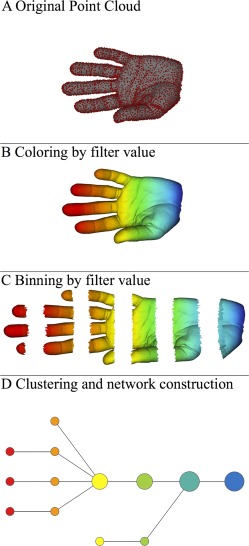
TDA pipeline. Visual depiction of TDA pipeline from point cloud to Reeb graph, reprinted from [Lum et al., 2013] in accordance with the Creative Commons license under which it was published (CC BY‐NC‐ND 3.0). [Color figure can be viewed in the online issue, which is available at http://wileyonlinelibrary.com.]

Overview of TDA

As with SVMs, the starting point for TDA is a data matrix whose m rows and n columns correspond to the variables of the study and their observed values; in the typical TDA data matrix, each column corresponds to a variable (e.g., voxel), and each row corresponds to an observation (e.g., subject). In geometric terms, we may interpret the n values in a row as giving the coordinates of a point in n‐dimensional space, and can thus interpret the m rows as m points (collectively called a point cloud) in space. In this way, we may also interpret the point cloud in Figure 1A in the shape of a hand as being a visual representation of a data matrix with thousands of rows and three columns, where the columns correspond to the x, y, and z coordinates of the points in the point cloud.

The first stage of TDA is to assign numerical values to each point in the point cloud, a process we refer to as selection of filter values; in Figure 1B, these values are represented by a color in the red‐blue spectrum. The next stage of TDA is to separate the point cloud into overlapping regions by separating the filter values into overlapping bins. For example, in Figure 1B we could view the filter values as indicating the distance from the tip of the middle finger as measured by a horizontal ruler, in which case we could then view the regions shown in Figure 1C as defined by the bins [0–1.5 in], [1–2.5 in], [2–3.5], [3–4.5], [4–5.5], [5–6.5]. The last stage of TDA is to represent each region from the previous stage by a dot, called a node, and then for each pair of regions that intersect, to connect the corresponding nodes by a line segment. Figure 1D shows the resulting Reeb graph, where the size and color of each node represent the number and “average” color of the points in the corresponding region. Note how the Reeb graph captures the underlying geometric structure of the hand, providing a schematic representation whose structural features correspond to real physical features, such as fingers, which also illustrates TDA's ability to highlight spectra and clusters within data, as described earlier. Note also that this construction does not involve multiple comparisons, and thus no correction for multiple comparisons is warranted.

Unlike the case of the hand, where our familiarity with its shape allows us to validate the Reeb graph of the corresponding point cloud, the “shape” of the point cloud corresponding to MRI data for our study population of young boys with FXS is not known to us a priori. To address this issue, we use TDA to identify subgroups purely on the basis of the MRI data, but then apply standard statistical tests to compare clinical data for these subgroups to provide confirmation they are clinically, as well as anatomically distinct.

Details of Reeb Graph Construction

As described earlier, we can interpret a subject's numerical data as the coordinates of a point in a high‐dimensional space S, referred to as subject space, and can thus recast the study population as a point cloud in subject space. In our case, we used the combined gray and white matter voxel data to create the subject space S, and then used the Iris software package to construct a Reeb graph of the data, so that we could explore the geometry of the resulting point cloud to identify its topological (i.e., shape) features [Lum et al., 2013] for an overview of Iris. These features would then correspond to anatomically defined subgroups of the study population, whose clinical profiles could then be compared and subjected to further analysis. In this subsection, we give a detailed description of the process used to construct a Reeb graph (Fig. 2 for a flowchart that summarizes this process).

Figure 2.

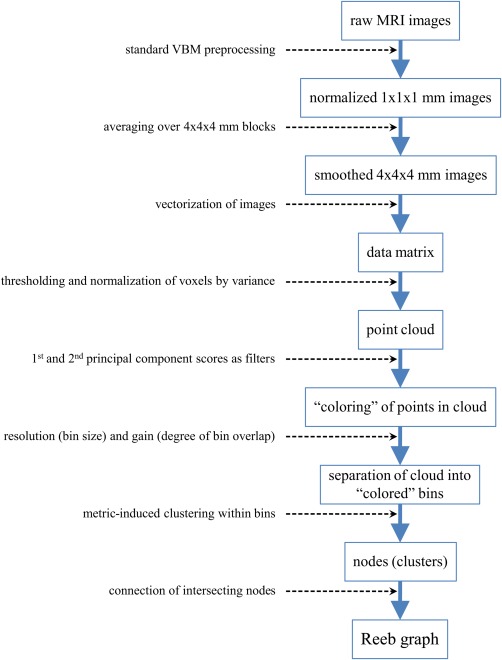
Reeb graph construction. Flowchart depicting the process used to construct a Reeb graph from raw MRI data. Note that the last four steps correspond to parts B, C, and D of Figure 1, with the last two steps corresponding to part D. [Color figure can be viewed in the online issue, which is available at http://wileyonlinelibrary.com.]

As noted above, Reeb graph construction begins, as do SVMs, with a data matrix. Since SVMs have already been used extensively in brain imaging studies, we followed the same approach to data matrix construction; namely, we combined the VBM‐preprocessed imaging data for the all subjects into a single matrix, with the data for each subject entered as a row of the data matrix. Specifically, we placed in each column the voxel intensity at a particular spatial location across all subjects. TThe process of converting a multidimensional object, like a 3D image, into an ordered list, like a row in a matrix, is known as vectorization, and is a common requirement of MVPA approaches [Pereira et al., 2009]. In principle, vectorization results in a loss of information about the spatial relationships between voxels, but in practice this loss does not appear to hamper the success of MVPA approaches in general, as evidenced by their use in numerous studies [Bray et al., 2009] for an extensive review of the use of MVPA in neuroimaging.

Before the preprocessed data were vectorized, the intensities for each subject's gray matter 1 × 1 × 1 mm³ voxel images were binned and averaged to produce corresponding gray 4 × 4 × 4 mm³ voxel images, and the same was done for each subject's 1 mm white matter images. This step was undertaken to both reduce noise in the 1 mm images by smoothing and for ease of computation. The voxels in each of these new 4 mm 3D images were then linearly ordered, so that each subject's gray and white matter images were converted into gray and white matter intensity vectors, which were then concatenated to produce a single, combined gray and white matter intensity vector. These combined intensity vectors were then used as rows to build a data matrix M of dimension (# subjects) × (# gray voxels + # white voxels).

Once the data matrix M is obtained, construction of a Reeb graph proceeds in several steps: (1) column selection, (2) metric selection, (3) filter selection, and finally (4) selection of values of the filter parameter called gain and resolution. The first step, column selection, is used to define the subject space S; this is done by selecting a subset of columns of M, whose size then determines the dimension of S. In our case, the columns of M correspond to voxels, and we chose to define S by selecting those voxels whose variance was at least 0.03. (In modulated and segmented images such as those utilized here [Hoeft et al., 2011], voxels intensities correspond to proportions of volume and thus range in value from 0 to 1). The next step, metric selection, is used to define distances within the subject space S, and thus provide a measure of similarity between subjects. Euclidean distance, a generalization of the usual distance between points P ₁ = (x ₁, y ₁) and P ₂ = (x ₂, y ₂) in the coordinate plane is only one of many choices for a metric on S.

$$d(P_1,P_2)=\sqrt{{(x_2-x_1)}^2+{(y_2-y_1)}^2}$$

Because we had no a priori basis for giving more weight in the analysis to a particular subset of the high‐variance voxels, we chose to standardize the voxel data before applying the Euclidean metric. The process of standardization, where data for each variable is first demeaned and then scaled to have variance 1, is a common statistical step taken in this context in order to give each variable equal weight in the subsequent analysis. In Iris, this is achieved by selecting the metric referred to as the variance‐normalized Euclidean metric.

The third step, filter selection, is in many ways the most critical choice made in the construction of a Reeb graph since it is the filters that transform the similarity information determined in the previous two steps into a visual representation that is easily grasped by the human eye, namely, a 2D rendering of a 3D graph (Fig. 3, below). Filters provide an alternative notion of similarity among subjects that is distinct from the one defined by the metric chosen for the subject space S, and together these two notions of similarity guide the construction of the vertices of the Reeb graph, in two stages. In the first stage, the filters are used to sort the subjects into bins based on similarity, where bin size is controlled by the resolution parameter from step 4. To capture the structure of variability among the subjects, we chose the first two principal component scores (PC1 and PC2) of the variance‐normalized data as our filters, so that two subjects were judged to be similar (i.e., shared the same bin) if both their PC1 and PC2 scores were sufficiently similar. In the second stage, the metric selected in step 2 is used to further cluster the subjects within each bin, so that two subjects within the same bin are merged into the same cluster if the distance between them is sufficiently small; each cluster obtained in this way is then viewed as a vertex of the Reeb graph. Finally, the edges of the graph are constructed as follows: Although bin size is governed by the resolution parameter, bins are allowed to overlap (i.e., share subjects) to an extent governed by the gain parameter, and this overlap may lead clusters from different bins to share subjects. Any two clusters (i.e., vertices) that share a subject are then joined by an edge. We may think of the resulting graph as a view of the data through a microscope, where gain and resolution play roles analogous to level of light and level of magnification. A group of edge‐connected vertices of the resulting Reeb graph may then serve as a candidate subgroup within the data (Fig. 3). In our case, a choice of parameter values that clearly decomposed the data into subgroups consisted of a gain of 4 for both PC1 and PC2, a resolution of 45 for PC1, and a resolution of 30 for PC2.

Figure 3.

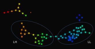
TDA results. An Iris rendering of a Reeb graph of the FXS data, with labels and ellipses added to indicate the subgroups LH and LL. Note that the size of each node corresponds to the number of subjects that were clustered to form that node, and that an edge between two nodes indicates that the corresponding clusters have a subject in common. The light blue node between the subgroups LH and LL is not included in either ellipse because it contains two subjects, one from each subgroup; nevertheless, the edges connected to this node indicate that each of the these subjects is also contained in a neighboring node within the appropriate subgroup. [Color figure can be viewed in the online issue, which is available at http://wileyonlinelibrary.com.]

Analysis of Behavioral Data

Once subgroups were identified with TDA based on neuroimaging data, we used standard t‐tests to compare subgroup differences on behavioral measures.

Univariate Analyses of Magnetic Resonance Images

Between subgroup contrasts using gray and white matter images were performed with FSL's randomize tool (http://fsl.fmrib.ox.ac.uk/fsl/fslwiki/Randomise) with 5000 permutations and threshold‐free cluster enhancement [Smith and Nichols, 2009] to correct for multiple comparisons. Images corresponding to P < 0.005 (corrected) were retained.

RESULTS

Multivariate Pattern Analysis

The parameter selections described above decomposed the data into two large subgroups and two smaller subgroups, as well as a single disconnected node containing just one subject (Fig. 3). In addition to classification by size, these subgroups could also be classified by PC1; indeed, size (small or large) and average value of PC1 (low or high) together clearly distinguished the four subgroups from one another. Accordingly, we will refer to the subgroups based on these Size and PC1 characteristics, respectively, as large‐low (LL, n = 19, mean [SD] age, 2.88 [0.67] years), large‐high (LH, n = 18, mean [SD] age, 3.13 [0.41] years), small‐low (SL, n = 4, mean [SD] age, 1.76 [0.20] years), and small‐high (SH, n = 10, mean [SD] age, 2.91 [0.55] years). Because of the limited sample size of the smaller subgroups (n = 4 and 10), and because SL and SH differ significantly in age from each other, our subsequent analyses focused on comparing the two larger subgroups (LL and LH).

Univariate VBM Results

Voxel‐wise comparison of the grey and white matter images for the LL and LH subgroups showed widespread significant and directionally uniform differences, with the LH subgroup consistently showing enlarged volumes relative to LL. Gray matter differences were bilaterally symmetric, encompassing regions of the cortex and of multiple subcortical structures as well as of the cerebellum. Aside from extensive midline cortical differences, differences were also found in the insular cortex, the inferior orbitofrontal cortex, the posterior region of the temporal lobe, and the inferior parietal lobule. Subcortical gray matter differences were found in the caudate, putamen, thalamus, hippocampus, and amygdala; cerebellar gray matter differences were observed in the superior surface of the cerebellum and the cerebellar vermis. White matter differences were also bilaterally symmetric, encompassing a large region of subcortical white matter as well as regions of cerebellar and brainstem white matter. The 2D gray matter images in the top portion of Figure 4 show those voxels that are significantly enlarged in LH relative to LL (P < 0.005) on a multiplanar image selected at a mid‐sagittal location; the collection of all such voxels across the whole brain are rendered as 3D images in the bottom portion of Figure 4, in Figure 5, and in Supporting Information Video 1. The corresponding white matter images appear in Figure 6 and in Supporting Information Video 2. All 3D images were produced with the 3D Viewer plug‐in [Schmid et al., 2010], as implemented in the Fiji distribution [Schindelin et al., 2012] of the ImageJ image‐processing software suite [Schneider et al., 2012].

Figure 4.

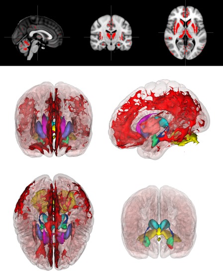
2D and 3D gray matter differences. Top: Red color indicates voxels where gray matter volume is significantly enlarged in the LH subgroup relative to LL (P < 0.005, corrected). Bottom: anterior, superior, and lateral views of 3D rendering of all such voxels, color‐coded by region: noninsular cortex (red), caudate (magenta), putamen (purple), insular cortex (peach), thalamus (cyan), hippocampus (blue), amygdala (green), cerebellum (yellow), and brain stem (lavender). The full MNI 152 cortex (pink) is included as a reference. In lower right view, cortical and anterior structures were removed to expose posterior structures, so that in addition to the superior surface of the cerebellum, a separate region of the cerebellar vermis is visible. [Color figure can be viewed in the online issue, which is available at http://wileyonlinelibrary.com.]

Figure 5.

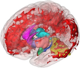
3D gray matter differences: oblique view. Oblique anterior‐superior‐lateral view of 3D rendering of all voxels where gray matter volume is significantly enlarged in the LH subgroup relative to LL (P < 0.005, corrected), color‐coded by region: noninsular cortex (red), caudate (magenta), putamen (purple), insular cortex (peach), thalamus (cyan), hippocampus (blue), amygdala (green), and cerebellum (yellow). The full MNI 152 cortex (pink) is included as a reference. [Color figure can be viewed in the online issue, which is available at http://wileyonlinelibrary.com.]

Figure 6.

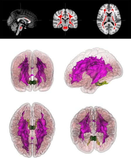
2D and 3D white matter differences. Top: Red color indicates voxels where white matter volume is significantly enlarged in the LH subgroup relative to LL (P < 0.005, corrected). Bottom: Anterior, superior, lateral, and oblique views of 3D rendering of all such voxels, color‐coded by region: subcortical white matter (magenta), cerebellar white matter (lime green), and brain stem white matter (dark green). The full MNI 152 cortex (pink) is included as a reference. In lower right, an oblique superior‐posterior view was used to highlight the separation between the subcortical and cerebellar/brain stem regions. [Color figure can be viewed in the online issue, which is available at http://wileyonlinelibrary.com.]

Behavioral Results

Comparison of key behavioral measures for the LL and LH subgroups showed significant differences across all of the standardized measures comprising the Mullen Scales of Early Learning (MSEL–Table 2; higher scores indicate higher cognitive function), as well as across all ADOS and ADI measures (Tables 3 and 4; lower scores indicate less severe symptoms) except those for play (ADOS, P = 0.0829) and repetitive or stereotyped behavior (ADOS, P = 0.0883; ADI, P = 0.368). All significant differences (P < 0.05) were coupled with effect sizes greater than 0.5 (Cohen's d), with large effect sizes for the MSEL Composite (0.95), Receptive Language (0.82), Visual Reception (0.82) standardized scores. These differences uniformly place the LH subgroup on the more severe (or lower functioning) end of the spectrum on every measure. Behavioral comparisons of LL and LH with SH, the larger of the two subgroups excluded from our analysis, can be found in Supporting Information Tables I–VI).

Table 2.

Mullen scales of early learning

Standardized subscale	LL mean(SD)	LH mean (SD)	Difference	P‐value	Cohen's d
Composite	58.68 (11.29)	50.67 (3.43)	8.02	0.004	0.95
Receptive Language	27.89 (10.65)	20.94 (2.04)	6.95	0.006	0.89
Visual Reception	28.89 (10.32)	22.11 (5.18)	6.78	0.008	0.82
Expressive Language	26.21 (8.84)	21.72 (3.61)	4.49	0.026	0.65
Fine Motor	23.37 (4.34)	20.50 (2.12)	2.87	0.043	0.58

Table 3.

Autism diagnostic observation schedule‐generic

Subscale	LL mean (SD)	LH mean (SD)	Difference	P‐value	Cohen's d
Social	5.00 (3.99)	7.83 (3.71)	−2.83	0.016	−0.73
Communication/Social	8.47 (6.02)	12.39 (4.96)	−3.92	0.019	−0.71
Communication	3.47 (2.20)	4.56 (1.65)	−1.08	0.049	−0.55
Stereotyped Behavior	1.53 (1.80)	2.28 (1.41)	−0.75	0.083	−0.46
Play	2.63 (1.34)	3.22 (1.26)	−0.59	0.088	−0.45

Table 4.

Autism diagnostic interview–revised

Subscale	LL mean (SD)	LH mean (SD)	Difference	P‐value	Cohen's d
Social	7.56 (4.88)	10.71 (5.46)	−3.15	0.041	−0.61
Communication (nonverbal)	7.81 (4.39)	10.19 (3.17)	−2.38	0.045	−0.62
Abnormal development	3.89 (1.02)	4.41 (0.80)	−0.52	0.050	−0.57
Communication (verbal)	3.67 (3.79)	10.00 (2.83)	−6.33	0.064	−1.88
Repetitive and stereotyped behavior	3.06 (1.80)	3.24 (1.30)	−0.18	0.368	−0.11

DISCUSSION

Although one might naturally expect variation within FXS at the “macro” level of behavior, our study suggests that FXS may lack homogeneity at the neurobiological level as well despite its single‐gene origin. Indeed, our results suggest that the LH and LL subgroups may correspond to separable phenotypes within FXS that have significantly different neuroanatomical and behavioral profiles. These subgroups accounted for a large proportion of 1‐ to 3‐year‐old boys with FXS in our sample (71%). It is interesting to note that the neuroanatomical and behavioral differences between LH and LL are analogs to differences previously noted to distinguish young children with FXS from typically‐developing children. Specifically, in addition to the LH subgroup scoring lower on measures of IQ and higher on measures of autism‐related behaviors, the regions of the brain that are enlarged in LH relative to LL (e.g., the caudate, putamen, and thalamus) are consistent with the regions reported to be enlarged in FXS relative to typically‐developing controls [Hazlett et al., 2012; Hoeft et al., 2008], with the notable exceptions of the amygdala and cerebellar vermis, which appear enlarged in LH relative to LL but reduced in FXS relative to typically‐developing controls. It is also potentially noteworthy that the LH subgroup shows enlarged volume of the middle cerebellar peduncles (MCP), white matter tracts that connect the cerebellum to the pons (Fig. 7). These same MCP tracts are also the location in which T2 hyperintensities occur in patients with fragile X tremor/ataxia syndrome (FXTAS), often referred as the “MCP sign” in males with the “premutation” form of the FMR1 gene mutation [Brunberg et al., 2002]. The significance of this finding in the LH subgroup and its possible association with neuroimaging findings in FXTAS is a potential area for future investigation.

Figure 7.

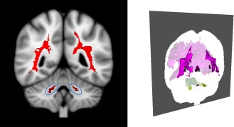
MCP sign and white matter differences. Left: Red color indicates voxels where white matter volume is significantly enlarged in the subgroup LH relative to LL (P < 0.005, corrected), and blue ellipses indicate region spatially analogs to the “MCP sign” in FXTAS. Right: Oblique posterior 3D view with the coronal slice of the left image placed in its correct orientation. Note that opacity of the slice dims the brightness of white matter anterior to the slice, so that the boundary between anterior and posterior white matter coincides with the regions shown in red in the left image. [Color figure can be viewed in the online issue, which is available at http://wileyonlinelibrary.com.]

As to a plausible explanation for the differences between LL and LH, one could speculate about the existence of a second genetic factor that, through its interaction with FMR1, leads to a bifurcation in the developmental trajectories of children with FXS. For example, a similar bifurcation has been suggested in 22q.11.2 deletion syndrome, where functional polymorphisms of the COMT gene may contribute to reduced prefrontal cortical gray matter and increased risk for developing psychosis [Gothelf et al., 2005]. Further evidence for gene interaction comes from studies of Fmr1 knockout mice, which show that differences in genetic background are associated to significant differences in social approach. Research designed to test this hypothesis could be carried out focusing on genotypic variations in signaling pathways known to interact with the FMR1 protein [Ascano et al., 2012]. Given that the data analyzed here are from the first time point in a longitudinal study of young boys with FXS [Hoeft et al., 2010], we also plan to perform TDA with data collected at 3–6 years of age in the same sample, as well as with data from an independent sample of adults with FXS. These future studies will also attempt to explore approaches that allow recovery of 3D structural information that is lost as a consequence of MRI image vectorization.

As noted in [Nicolau et al., 2011], the power of TDA for revealing the structure of high‐dimensional data lies in its origins within the field of topology, the area of mathematics that is specifically concerned with characterizing the shape of high‐dimensional geometric structures. The tools of topology allow TDA to drastically reduce the dimension of high‐dimensional datasets while at the same time shed light on critical aspects of their structure, accomplishing both without sacrificing subtle but important information that can easily be lost through standard approaches such as PCA and linkage‐based clustering. The advantage of using TDA over PCA alone can be easily seen in Figure 8, where the scatter plot of the same values of PC1 and PC2 used in our TDA to identify the subgroups LH and LL has no obvious structure. (Note that SVMs require a priori labels, and so would not be appropriate in the current context).

Figure 8.

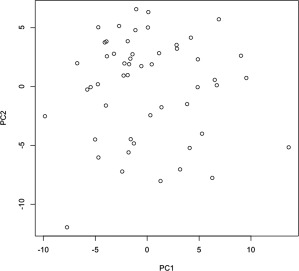
Unlabelled PCA scatter plot. Scatter plot of PC2 versus PC1 values for each subject, obtained from applying PCA to data matrix used in TDA (Compare with Supporting Information Fig. 1, in which the subgroups are color‐coded).

LIMITATIONS

Questions concerning inference and validation—natural questions that arise inevitably in connection to any novel analytical approach—are the subject of active ongoing research in TDA. Furthermore, the most direct means of validating our results, namely replication, is not one that is available to us at this time. As mentioned earlier, we do plan to extend our analysis to include data from the same children at later ages, which would provide confirmation of our findings as they apply specifically to our study population; however, replicating our finding in an independent population of children with FXS within the same age as our cohort is clearly a necessary future step in validating our approach.

CONCLUSIONS

As more attention is brought to bear on the limitations of behaviorally‐defined taxonomies of psychiatric disorders [Cross‐Disorder Group of the Psychiatric Genomics Consortium, 2013], the case for replacing these taxonomies with new approaches based on high‐dimensional, multi‐modal data becomes more compelling. By integrating behavioral data with imaging and genetic data, our ability to cut the landscape of neuropsychiatric disorders along its natural joints will likely be enhanced, thus improving our ability to identify the boundaries between disorders with greater neurobiological validity more accurately. TDA is one method that can contribute to this new approach to brain disorders.

Supporting information

Supplementary Information Figure 1.

Supplementary Information Tables 1‐6.

Supplementary Information Video 1.

Supplementary Information Video 1.

REFERENCES

- Abrahams BS, Geschwind DH (2008): Advances in autism genetics: on the threshold of a new neurobiology. Nat Rev Genet 9:341–355. [DOI] [PMC free article] [PubMed] [Google Scholar]
- Ascano M, Mukherjee N, Bandaru P, Miller JB, Nusbaum JD, Corcoran DL, Langlois C, Munschauer M, Dewell S, Hafner M, Williams Z, Ohler U, Tuschl T. (2012): FMRP targets distinct mRNA sequence elements to regulate protein expression. Nature 492:382. [DOI] [PMC free article] [PubMed] [Google Scholar]
- Bray S, Chang C, Hoeft F (2009): Applications of multivariate pattern classification analyses in developmental neuroimaging of healthy and clinical populations. Front Hum Neurosci 3:30. [DOI] [PMC free article] [PubMed] [Google Scholar]
- Brock M, Hatton D (2010): Distinguishing features of autism in boys with fragile X syndrome. J Intellect Disabil Res 54:894–905. [DOI] [PubMed] [Google Scholar]
- Brunberg JA, Jacquemont S, Hagerman RJ, Berry‐Kravis EM, Grigsby J, Leehey MA, Tassone F, Brown WT, Greco CM, Hagerman PJ (2002): Fragile X premutation carriers: Characteristic MR imaging findings of adult male patients with progressive cerebellar and cognitive dysfunction. Am J Neuroradiol 23:1757–1766. [PMC free article] [PubMed] [Google Scholar]
- Calhoun VD, Eichelel T, Adali T, Allen EA (2012): Decomposing the brain: components and modes, networks and nodes. Trends Cogn Sci 16:255–256. [DOI] [PMC free article] [PubMed] [Google Scholar]
- Carlsson G (2009): Topology and data. Bull. Am Math Soc (N.S.) 46:255–308. [Google Scholar]
- Cross‐Disorder Group of the Psychiatric Genomics Consortium (2013): Identification of risk loci with shared effects on five major psychiatric disorders: a genome‐wide analysis. Lancet 381:1371–1379. [DOI] [PMC free article] [PubMed] [Google Scholar]
- Fair DA, Bathula D, Nikolas MA, Nigg JT (2012): Distinct neuropsychological subgroups in typically developing youth inform heterogeneity in children with ADHD. Proc Natl Acad Sci USA 109:6769–6774. [DOI] [PMC free article] [PubMed] [Google Scholar]
- Gotham K, Pickles A, Lord C (2009): Standardizing ADOS scores for a measure of severity in autism spectrum disorders. J Autism Dev Disord 39:693–705. [DOI] [PMC free article] [PubMed] [Google Scholar]
- Gothelf D, Eliez S, Thompson T, Hinard C, Penniman L, Feinstein C, Kwon H, Jin S, Jo B, Antonarakis SE, Morris MA, Reiss AL. (2005): COMT genotype predicts longitudinal cognitive decline and psychosis in 22q11.2 deletion syndrome. Nat Neurosci 8:1500–1502. [DOI] [PubMed] [Google Scholar]
- Hazlett HC, Poe MD, Lightbody AA, Styner M, MacFall JR, Reiss AL, Piven J (2012): Trajectories of early brain volume development in fragile X syndrome and autism. J Am Acad Child Adolesc Psychiatry 51:921–933. [DOI] [PMC free article] [PubMed] [Google Scholar]
- Hoeft F, Lightbody AA, Hazlett HC, Patnaik S, Piven J, Reiss AL (2008): Morphometric spatial patterns differentiating boys with fragile X syndrome, typically developing boys, and developmentally delayed boys aged 1 to 3 years. Arch Gen Psychiatry 65:1087–1097. [DOI] [PMC free article] [PubMed] [Google Scholar]
- Hoeft F, Carter JC, Lightbody AA, Cody Hazlett H, Piven J, Reiss AL (2010): Region‐specific alterations in brain development in one‐ to three‐year‐old boys with fragile X syndrome. Proc Natl Acad Sci 107:9335–9339. [DOI] [PMC free article] [PubMed] [Google Scholar]
- Hoeft F, Walter E, Lightbody AA, Hazlett HC, Chang C, Piven J, Reiss AL (2011): Neuroanatomical differences in toddler boys with fragile X syndrome and idiopathic autism. Arch Gen Psychiatry 68:295–305. [DOI] [PMC free article] [PubMed] [Google Scholar]
- Jacquemont S, Curie A, des Portes V, Torrioli MG, Berry‐Kravis E, Hagerman RJ, Ramos FJ, Cornish K, He Y, Paulding C, Neri G, Chen F, Hadjikhani N, Martinet D, Meyer J, Beckmann JS, Delange K, Brun A, Bussy G, Gasparini F, Hilse T, Floesser A, Branson J, Bilbe G, Johns D, Gomez‐Mancilla B. (2011): Epigenetic modification of the FMR1 gene in fragile X syndrome is associated with differential response to the mGluR5 antagonist AFQ056. Sci Transl Med 3:64ra1. [DOI] [PubMed] [Google Scholar]
- Lord C, Rutter M, Couteur A (1994): Autism diagnostic interview‐revised: A revised version of a diagnostic interview for caregivers of individuals with possible pervasive developmental disorders. J Autism Dev Disord 24:659–685. [DOI] [PubMed] [Google Scholar]
- Lord C, Risi S, Lambrecht L, Cook EH, Leventhal BL, DiLavore PC, Pickles A, Rutter M (2000): The autism diagnostic observation schedule‐generic: A standard measure of social and communication deficits associated with the spectrum of autism. J Autism Dev Disord 30:205–223. [PubMed] [Google Scholar]
- Lum PY, Singh G, Lehman A, Ishkanov T, Vejdemo‐Johansson M, Alagappan M, Carlsson J, Carlsson G. (2013): Extracting insights from the shape of complex data using topology. Sci Rep 3:1236. [DOI] [PMC free article] [PubMed] [Google Scholar]
- Nicolau M, Levine AJ, Carlsson G (2011): Topology based data analysis identifies a subgroup of breast cancers with a unique mutational profile and excellent survival. Proc Natl Acad Sci 108:7265–7270. [DOI] [PMC free article] [PubMed] [Google Scholar]
- Pereira F, Mitchell T, Botvinick M (2009): Machine learning classifiers and fMRI: A tutorial overview. Neuroimage 45:S199–S209. [DOI] [PMC free article] [PubMed] [Google Scholar]
- Schindelin J, Arganda‐Carreras I, Frise E, Kaynig V, Longair M, Pietzsch T, Preibisch S, Rueden C, Saalfeld S, Schmid B, Tinevez JY, White DJ, Hartenstein V, Eliceiri K, Tomancak P, Cardona A. (2012): Fiji: An open‐source platform for biological‐image analysis. Nat Methods 9:676–682. [DOI] [PMC free article] [PubMed] [Google Scholar]
- Schmid B, Schindelin J, Cardona A, Longair M, Heisenberg M (2010): A high‐level 3D visualization API for Java and ImageJ. BMC Bioinformatics 11. [DOI] [PMC free article] [PubMed] [Google Scholar]
- Schneider CA, Rasband WS, Eliceiri KW (2012): NIH Image to ImageJ: 25 years of image analysis. Nat Methods 9:671–675. [DOI] [PMC free article] [PubMed] [Google Scholar]
- Smith SM, Nichols TE (2009): Threshold‐free cluster enhancement: Addressing problems of smoothing, threshold dependence and localisation in cluster inference. Neuroimage 44:83–98. [DOI] [PubMed] [Google Scholar]
- Wolff JJ, Bodfish JW, Hazlett HC, Lightbody AA, Reiss AL, Piven J (2012): Evidence of a distinct behavioral phenotype in young boys with fragile X syndrome and autism. J Am Acad Child Adolesc Psychiatry 51:1324–1332. [DOI] [PMC free article] [PubMed] [Google Scholar]
Associated Data
This section collects any data citations, data availability statements, or supplementary materials included in this article.
Supplementary Materials