

Abstract
Brain connectivity network derived from functional magnetic resonance imaging (fMRI) is becoming increasingly prevalent in the researches related to cognitive and perceptual processes. The capability to detect causal or effective connectivity is highly desirable for understanding the cooperative nature of brain network, particularly when the ultimate goal is to obtain good performance of control-patient classification with biological meaningful interpretations. Understanding directed functional interactions between brain regions via brain connectivity network is a challenging task. Since many genetic and biomedical networks are intrinsically sparse, incorporating sparsity property into connectivity modeling can make the derived models more biologically plausible. Accordingly, we propose an effective connectivity modeling of resting-state fMRI data based on the multivariate autoregressive (MAR) modeling technique, which is widely used to characterize temporal information of dynamic systems. This MAR modeling technique allows for the identification of effective connectivity using the Granger causality concept and reducing the spurious causality connectivity in assessment of directed functional interaction from fMRI data. A forward orthogonal least squares (OLS) regression algorithm is further used to construct a sparse MAR model. By applying the proposed modeling to mild cognitive impairment (MCI) classification, we identify several most discriminative regions, including middle cingulate gyrus, posterior cingulate gyrus, lingual gyrus and caudate regions, in line with results reported in previous findings. A relatively high classification accuracy of 91.89 % is also achieved, with an increment of 5.4 % compared to the fully-connected, non-directional Pearson-correlation-based functional connectivity approach.
Keywords: Effective connectivity, Functional magnetic resonance imaging (fMRI), Mild cognitive impairment (MCI), Orthogonal least squares (OLS), Sparse multivariate autoregressive (MAR) model, Support vector machines (SVMs)
Introduction
Recent research has identified that Mild cognitive impairment (MCI) is the clinical condition between normal aging and Alzheimer’s disease (AD), who experience memory loss, yet do not meet the currently accepted criteria for clinically probable AD (Petersen et al. 2001; Li et al. 2012a; Zhang et al. 2011; Zhang & Shen 2012). MCI is considered as an intermediate state of cognitive function between normal aging and very early dementia (Petersen et al. 1999). The most prominent feature of MCI is an acquired syndrome characterized by cognitive decline, which does not interfere notably with activities of daily living (Gauthier et al. 2006). In recent years, MCI has received considerable attention in clinical practice and research, since it could progress to Alzheimer’s disease (AD) at a relatively high rate of approximately 10 % to 15 % per year (Grundman et al. 2004; Liu et al. 2012). The estimated prevalence of MCI in population-based studies ranges from 10 to 20 % in persons older than 65 years of age (Petersen 2011). Some people with MCI remain stable or even return to normal over time, but more than half progress to dementia within 5 years (Petersen 2011). Thus, MCI is regarded as a risk state of dementia, and its identification could lead to possible prevention by controlling risk factors such as systolic hypertension (Gauthier et al. 2006; Zhou et al. 2011; Zhang et al. 2012).
Recently, the role of neuroimaging in predicting progression from MCI to AD has gained a great deal of attention (Fox et al. 2001). In cognitive neuroscience, there is a prominent goal for understanding the interactions between brain structures through the functional and effective connectivity of perceptual processes or cognitive tasks. Specifically, neuroimaging approaches, such as those based on functional magnetic resonance imaging (fMRI), have been widely employed to address questions of functional connectivity and inter-regional interactions (Valdes-Sosa et al. 2005; Horwitz and Smith 2008; Roebroeck et al. 2011; Richiardi et al. 2012; Shirer et al. 2012). Learning functional brain connectivity from neuroimaging data holds great promise for identifying image-based markers that can be used to distinguish diseases, e.g., AD and MCI, from normal controls. Many functional connectivity modeling methods have thus been proposed based on correlation analysis (Wang et al. 2007; Zeng et al. 2012). However, correlation analysis, which assesses zero-lag correlations of the neural connectivity between brain regions (White et al. 2013), only captures pairwise information and is unable to reveal the time-lagged relationships between different brain regions (Deshpande et al. 2013).
Different from functional connectivity, effective connectivity can be used to identify time-lagged relationships between different brain regions, and thus can better understand the interaction mechanisms within the brain networks. Therefore, investigating the directional causal interactions among brain regions in MCI or AD can supplement functional connectivity findings, and potentially may serve as a neural biomarker for the disorder (Deshpande et al. 2013). Investigation of causal interactions is commonly accomplished by using structure equation modeling or dynamic causal modeling, which requires strict a priori assumptions about the underlying connectional network and directional architecture (Friston et al. 2011; Bianchi et al. 2013). In contrast, multivariate autoregressive (MAR) modeling technique, which has been widely used for a large number of time series modeling (Martinez-Montes et al. 2004; Valdes-Sosa 2004; Valdes-Sosa et al. 2005; Deshpande et al. 2009), is used in this study to identify how different brain regions interact with each other in disease processes based on the fMRI data (Fan et al. 2007; Rajapakse and Zhou 2007). MAR modeling is regarded as an exploratory technique which does not require any prior hypothesis about the potential connectional structure. Moreover, it is capable of obtaining Granger causal influences between different brain regions by using the relatively shorter time series when compared to the existing methods (Deshpande et al. 2013). MAR approach has also been proven to be very useful for modeling the interacting patterns between genes from microarray gene expression data, which measures thousands of genes with sample size being no more than a few hundred (Shimamura et al. 2009).
Inferring effective brain connectivity from fMRI data for biologically more meaningful interpretation and better classification performance is a challenging task. Many spurious connectivity might be arisen due to the low frequency (<0.1Hz) spontaneous fluctuation of blood oxygen level dependent (BOLD) signals and the physiological noise such as cardiac and respiratory cycles. Supekar et al. (2008) suggested that sparse representation can be employed to elucidate robust connections of the brain since brain connectivity networks are indeed sparse (Sporns et al. 2000, 2004; Kotter and Stephan 2003; Sporns and Zwi 2004). Actually, the sparse representation correlates well with the fact that a brain region predominantly interacts with only a small number of other regions. Most of recent studies have focused on the undirected functional connectivity measured by the correlation of two activity time series of separated brain regions (Zeng et al. 2012). However, little is known about the effective connectivity in MCI or AD, including how their effective connectivity patterns (directional causal influence of one brain region over another) differ from healthy subjects based on mathematical modeling (Friston et al. 2011).
The focus of this work is to develop a generalized disease identification framework based on sparse effective connectivity among brain regions derived from the resting-state fMRI data by using the MAR approach and the idea of Granger causality (Granger 1969; Li et al. 2012b). Granger causality is used to investigate whether the prediction of the present value of one time series by its own past values can be significantly improved by also including the past values of other time series. The Granger causality measure is typically implemented via autoregressive (AR) modeling and has been shown to be a powerful and flexible tool for identifying the predictability of one neural time series from another (Ding et al. 2000; Li et al. 2012b). The goals in this study are threefold. First, based on a multiple-input multiple-output (MIMO) model, the model order of each fMRI time-series will be estimated, using a model order determination criterion, to identify the model order distribution of each region-of-interest (ROI) in MCI patients and normal controls. Moreover, according to the distribution of optimal model order, group difference will be evaluated to identify the most discriminative regions between MCI and normal control groups. Second, based on the determined model order, MAR modeling approach will then be used to construct the effective connectivity between brain regions. Specifically a forward orthogonal least square (OLS) algorithm will be employed to obtain a satisfactory and sparse representation that involves only a small number of regression terms in the MAR model. Finally, feature matrix, which is extracted from those discriminative regions, will be applied for MCI classification. Classification accuracy will be evaluated via a leave-one-out (LOO) cross-validation to ensure performance generalization on the small sample size.
Materials and Methods
Subjects
In this study, all the subjects used were recruited by the Duke UNC Brain Imaging and Analysis Centre (BIAC), Durham, North Carolina, USA. Experimental protocols have been approved by the institutional ethics board at Duke University Medical Centre in compliance with the Health Insurance Portability and Accountability Act, and written informed consent was obtained from all participants. Twelve MCI patients and 25 socio-demographically matched normal controls were included in this study. All the participants were examined by expert consensus panels at the Department of Psychiatry at Duke University Medical Centre and the Joseph and Kathleen Bryan Alzheimer’s Disease Research Centre (Bryan ADRC). Diagnosis was made by a board-certified neurologist based on a battery of general neurological examination, collateral and subject symptom, neuropsychological assessment evaluation and functional capacity reports. The neurophysiological battery the Bryan ADRC used was a Consortium to Establish a Registry in Alzheimer’s Disease (CERAD) which included: 1) Mini-Mental State Examination (MMSE); 2) immediate and delayed verbal memory (Logical Memory subtest of the Wechsler Memory Scale-Revised); 3) visual immediate memory (Benton Visual Retention Test); 4) verbal initiation/lexical fluency (Controlled Oral Word Association Test from the Multilingual Aphasia Examination); 5) attentional/executive functions (Trail Making Test, Symbol Digit Modality Test, Digit Span sub-test of the Wechsler Adult Intelligence Scale-Revised, and a separate ascending Digit Span task modeled after the Digit Ordering Test); 6) premorbid verbal ability (Shipley Vocabulary Test); 7) Finger Oscillation Grooved Pegboard; and 8) Self Rating of Memory Function.
Diagnosis for MCI patients confirmed if subjects met the criteria as follows: (1) age > 55 years and any race; (2) recent worsening of cognition, but still functioning independently; (3) Mini Mental State Examination (MMSE) score between 24 and 30; (4) score ≤–1.5 standard deviation (SD) on at least two Bryan ADRC cognitive battery memory tests for single domain amnestic MCI; or score ≤–1.5 SD on at least one of the formal memory tests and score ≤–1.5 SD on at least one other cognitive domain task for multi-domain MCI (e.g., language, visuospatial-processing, or judgment/executive function); (5) four or lower for baseline Hachinski score; (6) does not meet the DSM-IV-TR or NINCDS-ADRDA criteria for dementia; (7) no psychological symptoms or history of depression; (8) capacity to give informed consent and follow study procedures.
Criteria for normal controls are: (1) age > 55 years and any race; (2) adequate visual and auditory acuity to properly complete neuropsychological testing; (3) no self-report of neurological or depressive illness; (4) based on the Diagnostic Interview Schedule portion of the Duke Depression Evaluation Schedule, shows no evidence of depression; (5) normal score on a non-focal neurological examination; (6) a score>–1 SD on any formal memory tests and a score>–1 SD on any formal executive function or other cognitive test; (7) demonstrates a capacity to provide informed consent and follow study procedures. In order to minimize biases, participants were excluded from the study if they have: (1) any of the traditional MRI contraindications including pacemakers or foreign metallic implants; (2) a past head injury or neurological disorder associated with MRI abnormalities such as dementia, epilepsy, demyelinating diseases, brain tumors and Parkinson’s disease, etc.; (3) any intellectual or physical disability affecting completion of assessments; (4) documentation of other Axis I psychiatric disorders; (5) any prescription medication (or nonprescription drugs) with known neurological effects. Note that the diagnosis of all cases was made on clinical grounds without reference to MRI.
Data Acquisition and Pre-Processing
Data acquisition was conducted using a 3.0-T GE Sigma EXCITE scanner. Resting-state functional images of each subject were collected with the following parameters: repetition time (TR)=2,000 ms; echo time (TE)=32 ms; and flip angle=77°. The acquisition matrix is 64×64 with a rectangular field of view (FOV) 256×256 mm2, resulting in a voxel resolution of 4×4×4 mm3. Each fMRI volume has a total of 34 slices, collected using a SENSE inverse-spiral pulse sequence. Totally, one hundred fifty (150) fMRI volumes were acquired per scan and all subjects were requested to keep their eyes open and stared at a fixation cross in the middle of the screen during a 5 min scanning process. Details of demographic information of the participants are provided in Table 1.
Table 1.
Demographic and clinical information of the subjects involved in this study
| Group | MCI | Normal | p-value |
|---|---|---|---|
| No. of subjects (Male/Female) | 6/6 | 9/16 | – |
| Age (Mean ± SD) | 75.0 ± 8.0 | 72.9 ± 7.9 | 0.3598a |
| Years of education (Mean ± SD) | 18.0 ± 4.1 | 15.8 ± 2.4 | 0.0419a |
| MMSE (Mean ± SD) | 28.5 ± 1.5b | 29.3 ± 1.1 | 0.1201a |
The p value was obtained by two-sample two tailed t-test
One of the patients does not have MMSE score
Resting-state fMRI (R-fMRI) images were preprocessed using the Statistical Parametric Mapping 8 (SPM8) software package (SPM8, http://www.fil.ion.ucl.ac.uk.spm/software/SPM8). Specifically, for each subject, the first 10 fMRI volumes acquired were discarded for magnetization equilibrium. Slice timing correction was performed on the remaining 140 fMRI volumes before they were realigned using a least squares method and a 6-parameters spatial transformation (Friston et al. 1995). The first scan of reminding fMRI time series was co-registered to its high-resolution T1-weighted image, which was acquired during fMRI data acquisition. Other fMRI volumes of the same subject were then linearly aligned to its high-resolution T1-weighted image by using the same estimated deformation fields. These fMRI volumes were down-sampled to their original dimension (4×4×4 mm3) before effective connectivity estimation. On the other hand, automated anatomical labeling (AAL) atlas (Tzourio-Mazoyer et al. 2002) was registered to the high-resolution T1-weighted image of each subject by using the deformation fields estimated from a deformable registration method called HAMMER (Shen and Davatzikos 2002; Xue et al. 2006; Yang et al. 2008; Zacharaki et al. 2008; Qiao et al. 2009; Tang et al. 2009; Yap et al. 2009; Jia et al. 2010), before downsampling to have the same dimensionality as fMRI images. The mean fMRI time series of each region-of-interest (ROI) according to AAL atlas was then computed for each subject by averaging the fMRI time series over all voxels in each ROI. In this work, temporal band-pass filtering of frequency interval (0. 025≤f≤0.100) was performed because the fMRI dynamics of neuronal activities in this frequency interval are most salient. This frequency interval was further decomposed into five equally non-overlapping frequency sub-bands to extract complex and subtle pathology information associated with MCI, enabling a more frequency specific analysis for the regional mean time series (Wee et al. 2012a). Before the derivation of effective connectivity, regression of nuisance signals such as WM and ventricular signals and six head-motion profiles was implemented to reduce their effects. Given the controversy of removing the global signal in the preprocessing of R-fMRI data (Murphy et al. 2009), the global signal was not regressed out (Supekar et al. 2008; Lynall et al. 2010). It was found that the head-motion profiles were matched between the MCI and normal control groups (p≥0.218 in any direction).
Sparse MAR Model for Studying Effective Connectivity
MAR modeling technique is normally used to model multiple time series so that the vector of current values of all variables can be considered as a linear summation of previous activities. We present a MAR model fitting to fMRI time series for exploring the underlying latent neuronal interaction. Suppose that we have M fMRI time series which are generated from M variables (or M ROIs in our case) within a system with N time points, represented as y(t)=[y1(t),y2(t), ···,yn(t),…, yM(t)]T … RM×1(t=1,2, ···,N), and [yn(1), yn(2), …, yn(t), …, yn(N)] is the time series obtained from the n-th ROI. The MAR model of q-th order predicts the next value in the M-dimensional time series, y(t), as a linear combination of the q previous vector values
| (1) |
where A(i) ∈ RM×M (i=1,2, ···,q) is the MAR coefficients matrix, and E(t)=[e1(t),e2(t), ···,en(t), ···eM(t)]T is the residual vector, which is assumed to constitute a zero-mean multivariate Gaussian process with a certain covariance matrix. The model order q can be determined using Bayesian information criteria (BIC) (Schwarz 1978). From Eq. (1), the MAR model is actually a multiple linear regression accounting for a linear relationship between current measurements and the past measurements. Particularly, if the model order q is equal to 0, the MAR model in Eq. (1) is simplified to the partial correlation of current measurements from different brain regions, and the diagonal elements of A(0) are zero, thus having only the instantaneous cross-correlation but not the auto-correlation between the time series modeled.
The model in Eq. (1) can be written in the standard form of a multivariate linear regression model as follows:
| (2) |
where φ(t)=[y(t–1),y(t–2), ···,y(t–q)] is the q previous multivariate time series samples, and θ is a (q×M)×M matrix of MAR coefficients or weights.
In the following, a capital letter represents a matrix with components corresponding to the ROIs. If the n-th row of Y, X, and E are yn(t), φn(t) and en(t) (n=1,2, ···,M), respectively, and there are t=1,2, ···,N samples, we can then recast the dynamics of the network of regions as a multivariate regression model
| (3) |
where Y is a (N–q)×M matrix, X is a (N–q)×(q×M) matrix, θ is a (q×M)×q matrix, and E is a (N–q)×M matrix.
For the model described in Eq. (3), each row of Y corresponds to a typical scan of fMRI data, and each column indicates the time-series for each region. Figure 1 represents a schematic representation of Eq. (3). The original M-dimensional time series (Y) given in Fig. 1a is modeled as a MAR process (Xθ) plus residual error (E). θ characterizes the M-dimensional time series as a network of connection strengths between all possible pairs of elements in the original series. A schematic representation of θ is shown in Fig. 1b, which includes q layers. Each layer is a M × M matrix of weights. The diagonal entries are self-connections, while the connections between regions are shown as the off-diagonal entries. If there is dependence between two ROI regions (brain regions), the corresponding entries in the M × M matrix are nonzero.
Fig. 1.

Schematic representation of MAR modeling. a The M-dimensional ROIs time series Y is modeled as a MAR process (Xθ) plus residual error (E). b θ is a matrix including all the weights characterized by the interactions of M ROIs. θ consists of q layers, with each layer containing a M×M matrix of weights. The q layers of θ have been put in sequential order at the bottom of the Figure
MAR models quantify the linear dependence of one region upon all other regions in the network, and thus infer the effective connectivity. The weights in θ can be interpreted as the influence that each region has upon it. Dependence between pair of regions is reflected by a nonzero magnitude, while independence results in a zero weight. We choose MAR modeling to construct effective connectivity networks of cortical activity for several reasons. First, MAR model is a dynamical model that can capture the temporal information among all possible combinations of region pairs in the model. Second, many random processes can be well approximated by a sufficiently high order of autoregressive (AR) model. Finally, MAR model can measure the directed influence among brain regions based on the concept of Granger causality (Goebel et al. 2003; Harrison et al. 2003).
Many approaches have been proposed to address the sparse modeling problem. The OLS algorithm, which was initiated for nonlinear system identification, has been widely used for sparse data modeling and analysis (Billings et al. 1989; Chen et al. 1989; Billings and Wei 2007). This type of algorithm is simple and very efficient to yield sparse linear models with good generalization properties (Chen et al. 2003). The advantage of the OLS-type algorithms is that the widely used model selection methods, such as the Akaike information criterion (AIC) (Akaike 1974), Bayesian information criterion (BIC) (Schwarz 1978), and the modified generalized cross validation (GCV) (Billings and Wei 2007), can be employed and incorporated easily into the sparse modeling algorithm to produce sparse linear regression models with good generalization performance (Chen et al. 2004; Li et al. 2011). In this study, the OLS algorithm discussed in the literature (Billings and Wei 2007) is applied for sparse regression model in Eq. (3).
MAR Model Order Determination
When constructing an AR model, it is important to determine the optimal model order which best fits the data. The optimal model order can be regarded as the number of past data samples that are required to accurately predict the present value of the data.
In our study, Bayesian information criterion (BIC) (Schwarz 1978) is applied to determine the optimal model order of the MAR model. For each subject, the model order qn in Eq. (1) for the n-th ROI can be determined by minimizing the BIC value:
| (4) |
where qn is the optimal model order of the n-th ROI time series when it is represented by ROI time series of M ROIs, N is the length of the n-th time series, and mse indicates mean square error or sum of square residual, respectively.
If the range of q is known in Eq. (1), for example qmin ≤q ≤qmax, the optimal model order can be determined by minimizing the BIC. Previous studies (Li et al. 2011) suggested that qmax for fMRI time series can be set to be 10, which will thus be used in this paper. Also, qmin=0 is used in our study to estimate the optimal order of the MAR model. Then, statistical t-test can be performed to explore group difference in terms of model order distribution between MCI patients and normal controls. In this way, we can identify the brain regions with significant different MAR model orders between MCI patients and normal controls, which will be detailed below.
MAR Network Construction
The M-dimensional model in Eq. (1) provides the directed causal influence through the non-zero entries in the matrix of MAR coefficients. It is unlikely that any of its components or coefficients θ is exactly zero. Therefore, the researchers have to test statistically whether the entries of θ are vanishing (Ahmad et al. 2012). However, instead of inspecting MAR coefficients directly, in our work it is preferable to test the corresponding square correlation coefficients for measuring direct interaction strength between regions (Billings and Wei 2007). In the OLS-type algorithm, the error reduction ratio (ERR) criterion, which is equivalent to the squared correlation coefficient, is used to measure the significance of the candidate repressors (Billings et al. 1989). It has been shown that the OLS algorithms interfered by the ERR criterion can produce a satisfactory and sparse model with good generalization performance (Billings et al. 1989; Chen et al. 1989, 1991; Billings and Wei 2007; Wei and Billings 2007; Wei et al. 2009; Li et al. 2011a). The significance of candidate model regressors in Eq. (1) is measured based on ERR criterion. The effective connectivity between region m1 with time series xm1 = [ym1 (1), ym1 (2), ···, ym1 (N)]T and region m2 time series xm2 = [ym2 (1), ym2 (2), ···, ym2 (N)]T with N time points is defined as
| (5) |
where ‘T’ indicates that transpose of a vector. Similar to the commonly used standard Pearson correlation coefficient, function in Eq. (5) reflects the linear relationship between two vectors xm1 and xm2 All these C values are arranged in an effective connectivity matrix of size M×M for M-dimensional time series, where the matrix contains every possible connectivity of ROI pairs (Billings and Wei 2007).
Inter-Region Relationship Determination
To investigate the between-group (MCI group vs. normal control group) difference, the MAR model order of each ROI is determined using the BIC given in Eq. (4). We then perform two-sample two-tailed t-test to identify d regions that are significantly (p<0.05) different between MCI and normal control groups in terms of their optimal model order distributions. Based on the specific model orders determined for each clinical group, we explore the causal relationships of these d regions with other brain regions. Specifically, in MCI group with 12 subjects with the model order q = qI1, we build an effective connectivity matrix of size 12×116 for each of d regions. One-tailed one sample t-test with a p-value of 0.05 is then used to determine and assess the relationship, either zero-lagged correlation or directed causal influence, of each of d regions with all other brain regions. Similar procedures are repeated for normal group with 25 subjects with the model order q = qI0. Note that if q >0, there are causal relationships among brain regions, while there are only correlation relationships among brain regions if q=0.
Effective Connectivity Matrix Construction for Classification
For each subject, effective connectivity matrices of size d×116 are constructed for model orders qI1 and qI0, respectively, using the definition in Eq. (5). These two effective connectivity matrices are then combined to form a new connectivity matrix W of size (2×d)×116. Elements in the connectivity matrix W are then treated as the input features to the SVM classifier. Here, we treat the brain regions as a set of nodes and the correlation strengths as the signed, weighted edges connecting nodes. Fisher’s r-to-z transformation is applied to the elements of effective connectivity matrix to improve the normality of the strength coefficients as
| (6) |
where r is the strength of correlation coefficient and z is approximately a normal distribution with standard deviation and K is the number of ROIs in the whole brain. Note that the effective connectivity networks are represented in the form of z-maps.
Identification of Effective Connectivity with High Discriminative Power
We decompose fMRI time series into five frequency sub-bands and build network for each of them. For each frequency sub-band, all the elements in the feature matrix W are concatenated into a vector of size (2×4)×116=928. (Note that, as shown below, we will identify the four (4) most discriminative regions between MCI and normal control groups, and then we can construct two effective connectivity matrices of size (4×116) by using the optimal model orders of MCI and normal control groups, respectively. These two effective connectivity matrices can finally combined to form a feature matrix W of size (8×116), as mentioned above.) Then, the feature vectors of all five frequency bands of the same subject are further concatenated into a long feature vector of size 5×928=4,640. Due to its high dimensionality, we employ a hybrid feature selection method that combines the benefits of maximum-relevance and wrapper-based feature selection approaches to determine the most discriminant features (Wee et al. 2011). Relevancy of a feature to classification is quantified using the Pearson correlation coefficient between this feature and class label. From a subset of features with the highest Pearson correlation coefficient values, a set of most discriminant features are then selected using the SVM recursive feature elimination (SVM-RFE) algorithm (Guyon et al. 2002; Wee et al. 2012b, 2013). For removal of a particular feature, SVM-RFE is performed via a LOO procedure to minimize the generalization error and to select the optimal combination of features. These selected features are considered as the most discriminant features.
Support Vector Classification and Performance Evaluation
When the features with high discriminative power are selected, SVM with nonlinear kernel is employed to evaluate the discriminative power of the selected features derived from effective connectivity networks for MCI classification. The optimal SVM models as well as an unbiased estimation of the generation performance of the complete framework are obtained via a nested cross-validation scheme. In particular, two cross-validation loops are employed: the inner cross-validation loop is applied to determine the hyperparameters of the SVM models from a training set, while the outer cross-validation loop is used to evaluate the generalizability of SVM models using an independent validation sets. Due to our limited number of samples, we use a LOO cross-validation strategy to estimate the generalization ability of our classifier. The performance of a classifier can be quantified using the generalization rate based on the results of cross-validation. In the proposed framework, the SVM classifier with non-linear radial basis function (RBF) kernel is employed. A summary of the proposed MCI classification framework is shown graphically in Fig. 2.
Fig. 2.
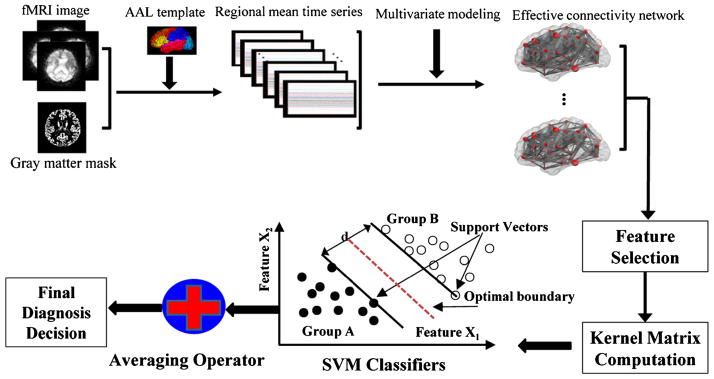
Schematic diagram of the proposed MCI classification framework
Experimental Results
MAR Model Order Determination
Based on the MAR modeling, we found that the MAR model order for each ROI is distributed between 0 and 1. The model orders of four regions (i.e., d=4), i.e., middle cingulate cortex (MCC), posterior cingulate gyrus (PCC), lingual gyrus (LING), and caudate (CAU), were found to be significantly different between MCI and normal control groups. Specifically, the model order is 0 and 1 for normal controls and MCI patients, respectively, in these four regions. Specially, in MCI patients, MCC and PCC regions are causally influenced by the inferior frontal gyrus (IFGtri) and anterior cingulate cortex (ACC) regions, respectively, while LING and CAU regions are only influenced by their own previous activity. Compared to MCI patients, the same four regions in the normal control group are closely related to their counter-hemisphere, i.e. left MCC vs. right MCC, left PCC vs. right PCC, left LING vs. right LING, and left CAU vs. right CAU, as shown in Fig. 3.
Fig. 3.

Between-group differences between MCI patients and normal controls in terms of effective connectivity and model order. a MCC and PCC regions are causally influenced by the IFGtri and ACC regions, respectively, while LING and CAU regions are directly influence by their own previous activity in MCI patients; b The same four regions are closely related to the counter-hemisphere in normal controls. MCC middle cingulate gyrus, PCC posterior cingulate gyrus, IFGtri inferior frontal gyrus, ACC anterior cingulate cortex, LING lingual gyrus, CAU caudate, NC normal control, R right, L left
Classification Results
By considering the four regions that show significant differences in terms of optimal model order between MCI patients (q=1) and normal controls (q=0), a feature matrix W of (2×4)×116 is constructed. In order to investigate the contribution of each frequency sub-band, we performed MCI classification using features derived from each individual frequency sub-band. The same leave-one-out (LOO) cross-validation classification procedure was applied to each individual frequency sub-band and then their classification performance is summarized in Table 2. It can be clearly observed that each individual frequency sub-band performed differently in MCI classification, indicating their different discriminative powers. Specifically, frequency Band1 ([0.025–0.039 Hz]) performed the best among all frequency sub-bands, although it still performed inferior than the proposed sparse MAR model with multi-spectrum method, both in terms of classification accuracy and AUC value. Other frequency sub-bands performed significantly worse than the Band1, in the order of Band2 ([0.039–0.054 Hz]), Band3 ([0.054–0.068 Hz]), Band4 ([0.068–0.082 Hz]), and Band5 ([0.082–0.100 Hz]). This result explains why only features from Band1, Band2, Band3, and Band4 were finally selected during the feature selection step.
Table 2.
Comparison of classification performance for multi- spectrum and individual frequency sub- bands (ACC = accuracy)
| Frequency band | ACC (%) | AUC |
|---|---|---|
| Band1 | 75.68 | 0.7300 |
| Band2 | 67.57 | 0.7233 |
| Band3 | 67.57 | 0.7067 |
| Band4 | 67.57 | 0.5033 |
| Band5 | 56.76 | 0.6300 |
| Multi-spectrum | 91.89 | 0.9033 |
Band1=[0.025–0.039 Hz], Band2=[0.039–0.054 Hz], Band3=[0.054–0.068 Hz], Band4=[0.068–0.082 Hz], and Band5=[0.082–0.10 Hz]
In the case of multi-spectrum classification, a total of 4,640 (5×(2×4)×116) features can be extracted from five frequency sub-bands. MCI classification performance of the proposed sparse representation method, which combines the optimal model order q=1 and q=0, is compared with 1) the effective connectivity with the MAR model order of q=1, 2) the partial correlation based connectivity with the MAR model of q=0, and 3) the non-directional Pearson correlation-based functional connectivity using multi-spectral network representation, with all their respective results summarized in Table 3. The proposed sparse MAR modeling with the combined model order approach yields the best classification of 91.89 %, which is at least 5.4 % higher than the Pearson-correlation-based and the partial-correlation-based methods. The classification accuracy by the effective connectivity approach with model order q=1 is 83.78 %, which is slightly inferior to the other comparison methods. A cross-validation estimation of the generalization performance shows an area of 0.9033 under the receiver operating characteristic curve (AUC) with the proposed method, indicating its excellent diagnostic power. Receiver operating characteristic (ROC) curves of all comparison methods are shown in Fig. 4.
Table 3.
Classification accuracies and AUC values for the sparse MAR and the correlation-based methods (ACC = accuracy; CI=95 % confidence intervals of AUC values)
| Approach | ACC (%) | AUC | CI |
|---|---|---|---|
| Non-directional Pearson correlation coefficients | 86.49 | 0.8630 | 0.6821~0.8325 |
| Partial correlation based connectivity with model order q=0 | 86.49 | 0.8100 | 0.6772~0.8224 |
| Effective connectivity with model order q=1 | 83.78 | 0.9033 | 0.6017~0.7947 |
| Sparse MAR model with optimal model order q=0 and 1 | 91.89 | 0.9033 | 0.7062~0.8614 |
Fig. 4.

ROC curves for the proposed and comparison methods
The Most Discriminant Effective Connectivities
Since the selected effective connectivities are different for each leave-one-out (LOO) cross-validation fold, those selected effective connectivities with the highest selected times are considered as the most discriminative connectivity features for MCI classification. The top 13 selected connectivity features, together with their selected frequencies, are listed in Table 4.
Table 4.
Top 13 selected effective connectivities by the proposed classification framework
| Selected ROI | Direction of effective connectivity | Neighbor of selected ROIs | No. of frequency |
|---|---|---|---|
| PCC R | ← | HIP L | 31 |
| PCC R | ↔ | SMG R | 21 |
| CAU L | ↔ | OFC R | 13 |
| MCC L | ↔ | MCC R | 12 |
| PCC R | ↔ | PCC L | 12 |
| MCC L | ← | ITG L | 12 |
| PCC R | ↔ | ITG L | 12 |
| LING L | ← | LING L | 11 |
| MCC L | ↔ | IPG L | 11 |
| PCC R | ← | SMG L | 11 |
| PCC R | ← | MTG L | 11 |
| PCC R | ↔ | PCNU L | 10 |
| CAU L | ↔ | CAU R | 10 |
where →: direction of causal influence; ↔: correlation of counter regions
HIP hippocampus, SMG supramarginalgyrus, OFC orbitofrontal cortex, ITG inferior temporal gyrus, IPG inferior parietal gyrus, MTG middle temporal pole, PCNU precuneus, R right, L left
Discussion
In this study, we propose a sparse multivariate modeling approach for identifying effective connectivity between brain regions. The proposed method is based on estimating MAR models by a two-stage process. First, model order of each ROI is determined by using the selection criteria of optimal model order. In the conventional MAR modeling, R-fMRI time series are normally modeled using a default model order of q=1 for all ROIs (Martinez-Montes et al. 2004; Valdes-Sosa 2004; Valdes-Sosa et al. 2005; Deshpande et al. 2009). It is worth noting that R-fMRI data with different repetition time (TR) were employed in these studies. For instance, R-fMRI data with TR of 2 s was used in (Deshpande et al. 2009), data with TR of 2.5 s was used in Martinez-Montes et al. (2004) and Valdes-Sosa (2004), and data with TR of 3 s was used in Valdes-Sosa et al. (2005), respectively. However, this model order does not guarantee the best fitting of R-fMRI time series at different brain regions since they may interact differently, particularly for the diseased individuals (Wang et al., 2007). Since the Granger causality is highly correlated with the TR value used during R-fMRI data acquisition, it is tremendously important to take into consideration the TR value when determining the optimal model order of MAR based on this time-lagged relationship. For instance, the optimal model order determined with TR of 2 s may be different from the optimal model order determined with TR of 2.5 s. Hence, it is important to determine the optimal model order for best fitting the R-fMRI time series of each ROI in different clinical groups, and uses this optimal model order to the R-fMRI data acquired with the same TR. Accordingly, we proposed to model the R-fMRI time series of each ROI using its optimal model order, where this optimal MAR modeling can better characterize the time series of each ROI, and potentially be used to improve patient-control identification accuracy. Second, due to the sparse nature of brain networks, we incorporate the forward OLS algorithm into MAR modeling to minimize spurious connections and physiological noise caused by cardiac and respiratory cycles. Specifically, we utilize OLS algorithm to identify the significant regressors in MAR model by measuring the direct interaction strength between pairwise regions based on the estimated optimal model order and ERR criterion. The details of estimation procedure of the OLS algorithm and ERR are presented in Appendix. Altered effective connectivities that are identified by the proposed method include four regions of MCC, PCC, LING and CAU. In particular, the classification accuracy of 91.89 % suggests that the effective connectivities between MCC, PCC, LING, CAU and other brain regions are significantly altered in MCI patients and hence can be used for the classification between MCI and normal controls.
Identifying Significant Between-Group Regions Using MAR Model Order
In previous studies (Martinez-Montes et al. 2004; Valdes-Sosa 2004; Valdes-Sosa et al. 2005; Deshpande et al. 2009), it is generally assumed that the MAR models with model order 1 fit well to the fMRI data. This assumption simplifies the description of models and methods. In fact, all software, which is developed for MAR modeling, has been designed to accommodate all model orders. It is found that the best MAR model order for different ROIs is 0 or 1. This result demonstrates that some ROIs are correlated with other regions, while other ROIs are causally influenced by other regions. This observation reveals a significantly different distribution of model order between MCI patients and normal controls. Particularly, we have found that the model order in the four regions, i.e., MCC, PCC, LING and CAU, is 1 for MCI patients while 0 for normal controls, which is not always equal to 1 as assumed in the literature (Martinez-Montes et al. 2004; Valdes-Sosa 2004; Valdes-Sosa et al. 2005). Model order q=0 indicates that each ROI just has a partial correlation with other regions, while the model order q=1 indicates that each ROI is causally influenced by other regions. The result of model order q=1 in these four regions indicates that these four brain regions may be causally influenced by other regions in MCI patients. These four regions have been reported to be associated with MCI (Chetelat et al. 2002; Greicius et al. 2003; Bai et al. 2008; Grambaite et al. 2011; Nickl-Jockschat et al. 2012).
The middle cingulate cortex (MCC) involves in understanding intention and actual social intention (Walter et al. 2004). Anderson et al. (2013) found that MCI patients are associated with disrupted connectivity associated with executive function, social cognition, and social interaction. Regional homogeneity analysis for the regional atrophy revealed decreased homogeneity in PCC region for MCI patients (De Vogelaere et al. 2012). Zhang et al. (2009) also demonstrated that in the early stage of AD, connectivities between PCC and ACC are disrupted. Decreased activity in these regions might be associated with alterations in episodic memory processing of early neurodegeneration (Greicius et al. 2004). On the other hand, significant abnormality of the resting-state connectivity related to the LING region has been reported in the literature (Saur et al. 2010), which may be associated with impaired attention and working memory in MCI/AD (Yetkin et al. 2006). Apostolova et al. (2010) reported that AD subjects with cognitive decline show preferential atrophy of the CAU, indicating that CAU atrophy can cause prefrontal cognitive deficits, disturbance of attention, and impaired recent and remote memory (Camicioli et al. 2009). Han et al. (2012) discovered smaller connectivity between cingulate cortex and CAU, and greater connectivity between cingulate cortex and IFGtri region in persons with MCI. Grambaite et al. (2011) found that WM tract degeneration in cingulate regions and cortical thinning in caudal frontal region are associated with executive impairment in MCI. MCI has been reported to be closely related with extensive GM atrophy, e.g., reduced GM concentration in LING, PCC, and bilateral CAU regions (Grambaite et al. 2011; Melzer et al. 2012). These findings imply that the brain activation of MCI patients in these four regions is different from the normal controls. In Fig. 3a, MCC and PCC regions are causally influenced by the IFGtri and ACC regions, respectively, while LING and CAU regions in MCI are influenced by their own previous activity. However, they are correlated with their counter hemisphere regions in normal controls as shown in Fig. 3b, where an arrow indicates the direction of causal influence and a bidirectional arrow indicates the correlation of counter hemisphere. All these findings may imply that the cognitive function deficits in MCI patients could be attributed to the connectivity abnormality in these four regions.
Functionally, compared to normal controls, Supekar et al. (2008) found that there is significantly lower regional connectivity and disrupted global functional organization in AD patients. This implies that cognitive decline in AD patients is associated with the disrupted functional connectivity in whole brain. Structurally, AD is associated with the atrophy in corpus callosum (CC), the crucial WM structure that plays the important role in communication between two cerebral hemispheres (Di Paola et al. 2010; Zhu et al. 2012). Compared to normal controls, Paola et al. (2010) found that the CC is significantly susceptible to atrophy in MCI patients, indicating deficit of between-hemisphere communication. We speculate that the asymmetric neuronal connectivity (i.e., asymmetry directed toward one hemisphere) observed in these four regions may disturb the performance of cognitive processing in MCI patients. Oertel et al. (2010) found that asymmetry for MCI and AD impeded the interaction between the hemispheres, which impaired the working efficiency of the brain. In this context, our finding further supports the assumption that AD and MCI is a disconnection syndrome.
Reliable Identification of MCI Patients
High classification accuracy of 91.89 % with sensitivity of 83.3 % and specificity of 96.0 % obtained by the proposed sparse MAR modeling with the combined optimal model orders indicates a significant improvement from the conventional approaches that use either the partial correlation-based connectivity with the MAR model order q=0, the effective connectivity with the model order q=1, or Pearson correlation based connectivity. The proposed method also shows a relatively high AUC value of 0.9033, indicating good diagnostic power, particularly in view of relatively small sample size available in this work. In most of the cases, simple connectivity description can only provide limited biophysical information for distinguishing MCI patients from normal controls, which is unable to provide good generalization power, as indicated by much smaller AUC values. Effective connectivity constructed by the proposed sparse MAR modeling approach, which uses the combined optimal model orders, is more effective in conveying relevant and subtle information, particularly for the purpose of classification.
Identifying Most Discriminant Effective Connectivities from Classification
Besides improvement on classification performance, it is important to identify which effective connectivities are potential biomarkers for MCI classification. Table 3 provides the top selected connectivities of brain regions, including MCC, PCC and CAU which are correlated by their counter regions, respectively, and LING which is causally influenced by its own previous activity.
It is found that PCC is causally influenced by the hippocampus gyrus (HIP), and middle temporal pole (MTG), while correlated with the supramarginal gyrus (SMG), inferior temporal gyrus (ITG), and precuneus (PCNU), which are the important components in default mode network (DMN) (Greicius et al. 2003). Previous studies also showed that AD patients are related to the abnormalities of DMN and these abnormalities could be served as biomarkers for the diagnosis and monitoring of MCI patients (Qi et al. 2010).
AD patients show disrupted connectivity between CAU and orbitofrontal cortex (OFC), parts of the decision-making network (Dai et al. 2009). This network plays an important role and has reciprocal connections with many brain regions that mediate the rewarding effects of decision-making (Bolla et al. 2003). Tekin et al. (2001) suggested that the disrupted connectivity between OFC and CAU regions was associated with deficits of decision-making. Abnormal connectivity between MCC and ITG regions found in our study was also reported in the literature (Tondelli et al. 2012). The attenuation of causal effects may contribute to the connectivity disruption in MCI patients (Miao et al. 2011).
Limitations and Future Directions
Pattern classification using fMRI data is a challenging task due to the high dimensionality of the data, noisy measurements, individual variability, and small available sample size. Our study demonstrates that the resting-state effective connectivity patterns can be used to distinguish MCI patients from normal controls with a relatively high accuracy and AUC value. However, there are some issues that may potentially influence the generalization performance of classifier, for instance, the selection of brain atlas (Smith et al. 2011). Different atlases with different levels (i.e., macro or microstructure) may have different impacts on the computed effective connectivity and thus the classification accuracy (Smith et al. 2011).
In the macro-scale connectivity analysis, the average of the BOLD signals over all voxels within each ROI is extracted as the representative time series for each ROI. The present study is on macro-level connectivity analysis, which explores and utilizes information flow between different brain regions. These macro-level mean time series are then applied to MAR modeling and Granger causality analysis. However, the strength of connectivity between voxels in different ROIs may be different, in which it might entail information loss (Sato et al. 2010). Thus, in the micro-level connectivity analysis, principal component analysis (PCA) was applied to obtain an ROI representative time series (Zhou et al. 2009). Recently, Leonardi et al. (2013) also suggested the application of PCA to extracting the principal eigen-time-series from ROIs for revealing the hidden patterns of coherent connectivity pattern. However, all the aforementioned approaches are mainly focused on the construction of dynamic functional connectivity network, without considering the directional and causality information between brain regions. On the other hand, in the proposed framework, we are indeed exploring how the time series of an ROI can be represented by the current and previous values of other ROIs, i.e., causal influence between ROIs. However, given the increasing evidence of dynamic functional connectivity during the resting, in our future work, we plan to include this dynamic property into our proposed framework for effective connectivity construction in the future.
For the sake of simplicity, the MAR modeling has been posited to be stationary and linear. Most fMRI connectivity studies, either explicitly or implicitly, assume the stationary and linearity of the resting-state fMRI signals (Smith 2012). In general, stationarity indicates that some statistics or model parameters of interest are time invariant. Linearity is referring to the output of node being a linear combination of its inputs. As quality and analysis approaches improve, it becomes more capable to model nonstationarities and nonlinearities, and we expect fMRI effective connectivity in modeling sophistication will become a tool for investigating disease mechanism in our future work.
Conclusion
This paper presents a novel statistical approach for estimation and inference of brain effective connectivity patterns from the resting-state fMRI data based on the sparse MAR modeling. We use MAR modeling to construct the effective connectivity patterns and examine the abnormalities in MCI patients as compared to normal controls. Significant group differences have been observed between MCI patients and normal controls using the constructed effective connectivity and the determination of optimal model order for each ROI. The impairment of effective connectivity in MCC, PCC, LING and CAU regions can serve as an important biomarker to distinguish MCI patients from normal controls. This sparse representation generates effective connectivity networks with identical network topology that enables better classification performance between subjects. The experiment results demonstrate that the proposed approach yields significantly improved classification performance when compared with the conventional correlation-based network. Moreover, the promising results indicate that the proposed classification framework can provide a complementary approach to clinical diagnosis of alterations in brain functions associated with cognitive impairment. Future investigations are needed to combine the resting-state effective connectivity with other neuroimaging evidence, such as structural abnormality, as a synthesized biomarker for more reliable clinical diagnosis.
Acknowledgments
This work was supported in part by NIH grants EB006733, EB008374, EB009634, AG041721, AG042599, NIA L30-AG029001, P30 AG028377-02, K23-AG028982, as well as National Alliance for Research in Schizophrenia and Depression Young Investigator Award (LW), Specialized Research Fund for the Doctoral Program of Higher Education (20131102120008), Project Sponsored by the Scientific Research Foundation for the Returned Overseas Chinese Scholars, State Education Ministry, and National Natural Science Foundation of China (81201049).
Appendix
The forward Orthogonal Least Squares algorithm and Error Reduction Ratios
Here, a brief introduction of the OLS algorithm is given as follows. Due to the use of the linear polynomial model in Eq. (3), matrix X is often referred to as the regression matrix. This regression matrix X can be orthogonally decomposed as
| (7) |
where V is an q×q unit upper triangular matrix and
| (8) |
is a (N–q)×q matrix with orthogonal columns that satisfy
| (9) |
and P is a positive diagonal matrix P=diag[p1, p2, ···,pd] with pi=ui,ui, where the symbol 〈·,·〉 denotes the inner product of two vectors, i.e.,
| (10) |
Equation (3) can now be expressed as
| (11) |
where G=[g1,g2, ···,gq]T is an auxiliary parameter vector, which can be calculated directly from Y and U by means of the property of orthogonality as , i = 1, 2, ···, q.
Rewrite Eq. (11) as
| (12) |
and calculate the inner product ui,Y, by substituting Y by Eq. (12), as
| (13) |
Calculate the inner product Y,Y from the Eq. (12)
| (14) |
Dividing both sides of Eq. (14) by Y,Y, then yields
| (15) |
The error reduction ratio ERRi due to ui can be presented by
| (16) |
The error reduction ratio often provides a simple and effective means for selecting a subset of significant terms from a large number of candidate terms in a forward regression manner. A term can be selected if it produces the largest value of ERRi among the rest of the candidate terms. The selection procedure will be terminated when
| (17) |
where ε is a desired tolerance, and this leads only to a subset model of q0 terms (q0≪q). The detailed procedure for derivation can be seen from Billings et al. (1989).
Footnotes
Information Sharing Statement
The data and computer code for the proposed algorithm are available upon request from the authors.
Contributor Information
Yang Li, Department of Radiology and BRIC, University of North Carolina at Chapel Hill, Chapel Hill, NC, USA. Department of Automation Science and Electrical Engineering, Beihang University, Beijing, China.
Chong-Yaw Wee, Department of Radiology and BRIC, University of North Carolina at Chapel Hill, Chapel Hill, NC, USA.
Biao Jie, Department of Radiology and BRIC, University of North Carolina at Chapel Hill, Chapel Hill, NC, USA.
Ziwen Peng, Department of Radiology and BRIC, University of North Carolina at Chapel Hill, Chapel Hill, NC, USA.
Dinggang Shen, Email: dgshen@med.unc.edu, Department of Radiology and BRIC, University of North Carolina at Chapel Hill, Chapel Hill, NC, USA. Department of Brain and Cognitive Engineering, Korea University, Seoul, Korea.
References
- Ahmad F, Maqbool M, Kim E, Park H, Kim DE. An efficient method for effective connectivity of brain regions. Concepts in Magnetic Resonance Part A. 2012;40:14–24. [Google Scholar]
- Akaike H. New look at statistical—model identification. IEEE Transactions on Automatic Control. 1974;19:716–723. [Google Scholar]
- Anderson RJ, Simpson AC, Channon S, Samuel M, Brown RG. Social problem solving, social cognition, and mild cognitive impairment in Parkinson’s disease. Behavioral Neuroscience. 2013;127:184–192. doi: 10.1037/a0030250. [DOI] [PubMed] [Google Scholar]
- Apostolova LG, Beyer M, Green AE, Hwang KS, Morra JH, Chou YY, et al. Hippocampal, caudate, and ventricular changes in Parkinson’s disease with and without dementia. Movement Disorders. 2010;25:687–695. doi: 10.1002/mds.22799. [DOI] [PMC free article] [PubMed] [Google Scholar]
- Bai F, Zhang Z, Yu H, Shi Y, Yuan Y, Zhu W, et al. Default-mode network activity distinguishes amnestic type mild cognitive impairment from healthy aging: a combined structural and resting-state functional MRI study. Neuroscience Letters. 2008;438:111–115. doi: 10.1016/j.neulet.2008.04.021. [DOI] [PubMed] [Google Scholar]
- Bianchi AM, Marchetta E, Tana MG, Tettamanti M, Rizzo G. Frequency-based approach to the study of semantic brain networks connectivity. Journal of Neuroscience Methods. 2013;212:181–189. doi: 10.1016/j.jneumeth.2012.10.005. [DOI] [PubMed] [Google Scholar]
- Billings SA, Wei HL. Sparse model identification using a forward orthogonal regression algorithm aided by mutual information. IEEE Transactions on Neural Networks. 2007;18:306–310. doi: 10.1109/TNN.2006.886356. [DOI] [PubMed] [Google Scholar]
- Billings SA, Chen S, Korenberg MJ. Identification of MIMO non-linear systems using a forward-regression orthogonal estimator. International Journal of Control. 1989;49:2157–2189. [Google Scholar]
- Bolla KI, Eldreth DA, et al. Orbitofrontal cortex dysfunction in abstinent cocaine abusers performing a decision-making task. NeuroImage. 2003;19:1085–1094. doi: 10.1016/s1053-8119(03)00113-7. [DOI] [PMC free article] [PubMed] [Google Scholar]
- Camicioli R, Gee M, et al. Voxel-based morphometry reveals extra-nigral atrophy patterns associated with dopamine refractory cognitive and motor impairment in parkinsonism. Parkinsonism & Related Disorders. 2009;15:187–195. doi: 10.1016/j.parkreldis.2008.05.002. [DOI] [PubMed] [Google Scholar]
- Chen S, Billings SA, et al. Orthogonal least-squares methods and their application to non-linear system-identification. International Journal of Control. 1989;150:1873–1896. [Google Scholar]
- Chen S, Cowan CFN, et al. Orthogonal least-squares learning algorithm for radial basis function networks. IEEE Transactions on Neural Networks. 1991;2:302–309. doi: 10.1109/72.80341. [DOI] [PubMed] [Google Scholar]
- Chen S, Hong X, et al. Sparse kernel regression modeling using combined locally regularized orthogonal least squares and D-optimality experimental design. IEEE Transactions on Automatic Control. 2003;48:1029–1036. [Google Scholar]
- Chen S, Hong X, et al. Sparse modeling using orthogonal forward regression with PRESS statistic and regularization. IEEE Transactions on Systems Man and Cybernetics Part B-Cybernetics. 2004;34:898–911. doi: 10.1109/tsmcb.2003.817107. [DOI] [PubMed] [Google Scholar]
- Chetelat G, Desgranges B, et al. Mapping gray matter loss with voxel-based morphometry in mild cognitive impairment. Neuroreport. 2002;13:1939–1943. doi: 10.1097/00001756-200210280-00022. [DOI] [PubMed] [Google Scholar]
- Dai W, Lopez OL, et al. Mild cognitive impairment and Alzheimer disease: patterns of altered cerebral blood flow at MR imaging. Radiology. 2009;250:856–866. doi: 10.1148/radiol.2503080751. [DOI] [PMC free article] [PubMed] [Google Scholar]
- Deshpande G, LaConte S, James GA, Peltier S, Hu X. Multivariate Granger causality analysis of fMRI data. Human Brain Mapping. 2009;30:1361–1373. doi: 10.1002/hbm.20606. [DOI] [PMC free article] [PubMed] [Google Scholar]
- Deshpande G, Libero LE, Sreenivasan KR, Deshpande HD, Kana RK. Identification of neural connectivity signatures of autism using machine learning. Frontiers in Human Neuroscience. 2013;7:670. doi: 10.3389/fnhum.2013.00670. [DOI] [PMC free article] [PubMed] [Google Scholar]
- De Vogelaere, Santens FP, et al. Altered default-mode network activation in mild cognitive impairment compared with healthy aging. Neuroradiology. 2012;54:1195–1206. doi: 10.1007/s00234-012-1036-6. [DOI] [PubMed] [Google Scholar]
- Ding MZ, Bressler SL, et al. Short-window spectral analysis of cortical event-related potentials by adaptive multivariate autoregressive modeling: data preprocessing, model validation, and variability assessment. Biological Cybernetics. 2000;83:35–45. doi: 10.1007/s004229900137. [DOI] [PubMed] [Google Scholar]
- Di Paola, Iulio MFD, et al. When, where, and how the corpus callosum changes in MCI and AD A multimodal MRI study. Neurology. 2010;74:1136–1142. doi: 10.1212/WNL.0b013e3181d7d8cb. [DOI] [PubMed] [Google Scholar]
- Fan Y, Rao H, Hurt H, Giannetta J, Korczykowski M, et al. Multivariate examination of brain abnormality using both structural and functional MRI. NeuroImage. 2007;36:1189–1199. doi: 10.1016/j.neuroimage.2007.04.009. [DOI] [PubMed] [Google Scholar]
- Fox NC, Crum WR, et al. Imaging of onset and progression of Alzheimer’s disease with voxel-compression mapping of serial magnetic resonance images. Lancet. 2001;358:201–205. doi: 10.1016/S0140-6736(01)05408-3. [DOI] [PubMed] [Google Scholar]
- Friston KJ, Frith CD, et al. Characterizing dynamic brain responses with fMRI—a multivariate approach. NeuroImage. 1995;2:166–172. doi: 10.1006/nimg.1995.1019. [DOI] [PubMed] [Google Scholar]
- Friston KJ, Li BJ, Daunizeau J, Stephan KE. Network discovery with DCM. NeuroImage. 2011;56:1202–1221. doi: 10.1016/j.neuroimage.2010.12.039. [DOI] [PMC free article] [PubMed] [Google Scholar]
- Gauthier S, Reisberg B, et al. Mild cognitive impairment. Lancet. 2006;367:1262–1270. doi: 10.1016/S0140-6736(06)68542-5. [DOI] [PubMed] [Google Scholar]
- Goebel R, Roebroeck A, et al. Investigating directed cortical interactions in time-resolved fMRI data using vector autoregressive modeling and Granger causality mapping. Magnetic Resonance Imaging. 2003;21:1251–1261. doi: 10.1016/j.mri.2003.08.026. [DOI] [PubMed] [Google Scholar]
- Grambaite R, Selnes P, et al. Executive dysfunction in mild cognitive impairment is associated with changes in frontal and cingulate white matter tracts. Journal of Alzheimer’s Disease. 2011;27:453–462. doi: 10.3233/JAD-2011-110290. [DOI] [PubMed] [Google Scholar]
- Granger CWJ. Investigating causal relations by econometric models and cross-spectral methods. Econometrica. 1969;37:414–420. [Google Scholar]
- Greicius MD, Krasnow B, et al. Functional connectivity in the resting brain: a network analysis of the default mode hypothesis. Proceedings of the National Academy of Sciences of the United States of America. 2003;100:253–258. doi: 10.1073/pnas.0135058100. [DOI] [PMC free article] [PubMed] [Google Scholar]
- Greicius MD, Srivastava G, et al. Default-mode network activity distinguishes Alzheimer’s disease from healthy aging: evidence from functional MRI. Proceedings of the National Academy of Sciences of the United States of America. 2004;101:4637–4642. doi: 10.1073/pnas.0308627101. [DOI] [PMC free article] [PubMed] [Google Scholar]
- Grundman M, Petersen RC, et al. Mild cognitive impairment can be distinguished from Alzheimer disease and normal aging for clinical trials. Archives of Neurology. 2004;61:59–66. doi: 10.1001/archneur.61.1.59. [DOI] [PubMed] [Google Scholar]
- Guyon I, Weston J, et al. Gene selection for cancer classification using support vector machines. Machine Learning. 2002;46:389–422. [Google Scholar]
- Han SD, Arfanakis K, et al. Functional connectivity variations in mild cognitive impairment: associations with cognitive function. Journal of the International Neuropsychological Society. 2012;18:39–48. doi: 10.1017/S1355617711001299. [DOI] [PMC free article] [PubMed] [Google Scholar]
- Harrison L, Penny WD, et al. Multivariate autoregressive modeling of fMRI time series. NeuroImage. 2003;19:1477–1491. doi: 10.1016/s1053-8119(03)00160-5. [DOI] [PubMed] [Google Scholar]
- Horwitz B, Smith JF. A link between neuroscience and informatics: large-scale modeling of memory processes. Methods. 2008;44:338–347. doi: 10.1016/j.ymeth.2007.02.007. [DOI] [PMC free article] [PubMed] [Google Scholar]
- Jia H, Wu G, Wang Q, Shen D. ABSORB: Atlas building by self-organized registration and bundling. NeuroImage. 2010;51:1057–1070. doi: 10.1016/j.neuroimage.2010.03.010. [DOI] [PMC free article] [PubMed] [Google Scholar]
- Kotter R, Stephan KE. Network participation indices: characterizing componet roles for information processing in neural networks. Neural Networks. 2003;16:1261–1275. doi: 10.1016/j.neunet.2003.06.002. [DOI] [PubMed] [Google Scholar]
- Leonardi N, Richiardi J, Gschwind M, Simioni S, Annoni JM, et al. Principal components of functional connectivity: a new approach to study dynamic brain connectivity during rest. NeuroImage. 2013;83:937–950. doi: 10.1016/j.neuroimage.2013.07.019. [DOI] [PubMed] [Google Scholar]
- Li X, Coyle D, et al. A model selection method for nonlinear system identification based fMRI effective connectivity analysis. IEEE Transactions on Medical Imaging. 2011;30:1365–1380. doi: 10.1109/TMI.2011.2116034. [DOI] [PubMed] [Google Scholar]
- Li Y, Wei HL, et al. Identification of time-varying systems using multi-wavelet basis functions. IEEE Transactions on Control Systems Technology. 2011a;19:656–663. [Google Scholar]
- Li Y, Wei HL, et al. Time-varying model identification for time-frequency feature extraction from EEG data. Journal of Neuroscience Methods. 2011b;196:151–158. doi: 10.1016/j.jneumeth.2010.11.027. [DOI] [PubMed] [Google Scholar]
- Li Y, Wang Y, Wu G, Shi F, Zhou L, et al. Discriminant analysis of longitudinal cortical thickness changes in Alzheimer’s disease using dynamic and network features. Neurobiol Aging. 2012a;33:427.e415–427.e430. doi: 10.1016/j.neurobiolaging.2010.11.008. [DOI] [PMC free article] [PubMed] [Google Scholar]
- Li Y, Wei HL, et al. Time-varying linear and nonlinear parametric model for Granger causality analysis. Physical Review E. 2012b;85(4) doi: 10.1103/PhysRevE.85.041906. [DOI] [PubMed] [Google Scholar]
- Liu M, Zhang D, Shen D. Ensemble sparse classification of Alzheimer’s disease. NeuroImage. 2012;60:1106–1116. doi: 10.1016/j.neuroimage.2012.01.055. [DOI] [PMC free article] [PubMed] [Google Scholar]
- Lynall ME, Bassett DS, et al. Functional connectivity and brain networks in schizophrenia. Journal of Neuroscience. 2010;30:9477–9487. doi: 10.1523/JNEUROSCI.0333-10.2010. [DOI] [PMC free article] [PubMed] [Google Scholar]
- Martinez-Montes E, Valdes-Sosa PA, et al. Concurrent EEG/fMRI analysis by multiway partial least squares. NeuroImage. 2004;22:1023–1034. doi: 10.1016/j.neuroimage.2004.03.038. [DOI] [PubMed] [Google Scholar]
- Melzer TR, Watts R, et al. Grey matter atrophy in cognitively impaired Parkinson’s disease. Journal of Neurology, Neurosurgery and Psychiatry. 2012;83:188–194. doi: 10.1136/jnnp-2011-300828. [DOI] [PubMed] [Google Scholar]
- Miao X, Wu X, et al. Altered connectivity pattern of hubs in default-mode network with Alzheimer’s disease: an granger causality modeling approach. PLoS ONE. 2011;6:e25546. doi: 10.1371/journal.pone.0025546. [DOI] [PMC free article] [PubMed] [Google Scholar]
- Murphy K, Birn RM, et al. The impact of global signal regression on resting state correlations: are anti-correlated networks introduced? NeuroImage. 2009;44:893–905. doi: 10.1016/j.neuroimage.2008.09.036. [DOI] [PMC free article] [PubMed] [Google Scholar]
- Nickl-Jockschat T, Kleiman A, et al. Neuroanatomic changes and their association with cognitive decline in mild cognitive impairment: a meta-analysis. Brain Structure & Function. 2012;217:115–125. doi: 10.1007/s00429-011-0333-x. [DOI] [PMC free article] [PubMed] [Google Scholar]
- Oertel V, Knoechel C, et al. Reduced laterality as a trait marker of schizophrenia-evidence from structural and functional neuroimaging. Journal of Neuroscience. 2010;30:2289–2299. doi: 10.1523/JNEUROSCI.4575-09.2010. [DOI] [PMC free article] [PubMed] [Google Scholar]
- Petersen RC. Mild cognitive impairment. New England Journal of Medicine. 2011;364:2227–2234. doi: 10.1056/NEJMcp0910237. [DOI] [PubMed] [Google Scholar]
- Petersen RC, Smith GE, et al. Mild cognitive impairment—clinical characterization and outcome. Archives of Neurology. 1999;56:303–308. doi: 10.1001/archneur.56.3.303. [DOI] [PubMed] [Google Scholar]
- Petersen RC, Doody R, Kurz A, et al. Current concepts in mild cognitive impairment. Archives of Neurology. 2001;58:1985–1992. doi: 10.1001/archneur.58.12.1985. [DOI] [PubMed] [Google Scholar]
- Qi Z, Wu X, et al. Impairment and compensation coexist in amnestic MCI default mode network. NeuroImage. 2010;50:48–55. doi: 10.1016/j.neuroimage.2009.12.025. [DOI] [PubMed] [Google Scholar]
- Qiao H, Zhang H, Zheng Y, Ponde DE, Shen D, et al. Embryonic stem cell grafting in normal and infarcted myocardium: serial assessment with MR imaging and PET dual detection. Radiology. 2009;250:821–829. doi: 10.1148/radiol.2503080205. [DOI] [PMC free article] [PubMed] [Google Scholar]
- Rajapakse JC, Zhou J. Learning effective brain connectivity with dynamic Bayesian networks. NeuroImage. 2007;37:749–760. doi: 10.1016/j.neuroimage.2007.06.003. [DOI] [PubMed] [Google Scholar]
- Richiardi J, Gschwind M, Simioni S, Annoni JM, Greco B, Hagmann P, et al. Classifying minimally disabled multiple sclerosis patients from resting state functional connectivity. NeuroImage. 2012;62:2021–2033. doi: 10.1016/j.neuroimage.2012.05.078. [DOI] [PubMed] [Google Scholar]
- Roebroeck A, Formisano E, et al. The identification of interacting networks in the brain using fMRI: Model selection, causality and deconvolution. NeuroImage. 2011;58:296–302. doi: 10.1016/j.neuroimage.2009.09.036. [DOI] [PubMed] [Google Scholar]
- Sato JR, Fujita A, Cardoso EF, Thomaz CE, Brammer MJ, Amaro E. Analyzing the connectivity between regions of interest: an approach based on cluster Granger causality for fMRI data analysis. NeuroImage. 2010;52:1444–1455. doi: 10.1016/j.neuroimage.2010.05.022. [DOI] [PubMed] [Google Scholar]
- Saur R, Milian M, et al. Cortical activation during clock reading as a quadratic function of dementia state. Journal of Alzheimer’s Disease. 2010;22:267–284. doi: 10.3233/JAD-2010-091390. [DOI] [PubMed] [Google Scholar]
- Schwarz G. Estimating dimension of a model. Annals of Statistics. 1978;6:461–464. [Google Scholar]
- Shen DG, Davatzikos C. HAMMER: hierarchical attribute matching mechanism for elastic registration. IEEE Transactions on Medical Imaging. 2002;21:1421–1439. doi: 10.1109/TMI.2002.803111. [DOI] [PubMed] [Google Scholar]
- Shimamura T, Imoto S, et al. Recursive regularization for inferring gene networks from time-course gene expression profiles. BMC Systems Biology. 2009;3 doi: 10.1186/1752-0509-3-41. [DOI] [PMC free article] [PubMed] [Google Scholar]
- Shirer WR, Ryali S, Rykhlevskaia E, Menon V, Greicius MD. Decoding subject-driven cognitive states with whole-brain connectivity patterns. Cerebral Cortex. 2012;22:158–165. doi: 10.1093/cercor/bhr099. [DOI] [PMC free article] [PubMed] [Google Scholar]
- Smith SM. The future of FMRI connectivity. NeuroImage. 2012;62:1257–1266. doi: 10.1016/j.neuroimage.2012.01.022. [DOI] [PubMed] [Google Scholar]
- Smith SM, Miller KL, et al. Network modelling methods for FMRI. NeuroImage. 2011;54:875–891. doi: 10.1016/j.neuroimage.2010.08.063. [DOI] [PubMed] [Google Scholar]
- Sporns O, Zwi JD. The small world of the cerebral cortex. Neuroinformatics. 2004;2:145–162. doi: 10.1385/NI:2:2:145. [DOI] [PubMed] [Google Scholar]
- Sporns O, Tononi G, et al. Theoretical neuroanatomy: relating anatomical and functional connectivity in graphs and cortical connection matrices. Cerebral Cortex. 2000;10:127–141. doi: 10.1093/cercor/10.2.127. [DOI] [PubMed] [Google Scholar]
- Sporns O, Chialvo DR, et al. Organization, development and function of complex brain networks. Trends in Cognitive Sciences. 2004;8:418–425. doi: 10.1016/j.tics.2004.07.008. [DOI] [PubMed] [Google Scholar]
- Supekar K, Menon V, et al. Network analysis of intrinsic functional brain connectivity in Alzheimer’s disease. PLoS Computational Biology. 2008;4(6) doi: 10.1371/journal.pcbi.1000100. [DOI] [PMC free article] [PubMed] [Google Scholar]
- Tang S, Fan Y, Wu G, Kim M, Shen D. RABBIT: Rapid alignment of brains by building intermediate templates. NeuroImage. 2009;47:1277–1287. doi: 10.1016/j.neuroimage.2009.02.043. [DOI] [PMC free article] [PubMed] [Google Scholar]
- Tekin S, Mega MS, et al. Orbitofrontal and anterior cingulate cortex neurofibrillary tangle burden is associated with agitation in Alzheimer disease. Annals of Neurology. 2001;49:355–361. [PubMed] [Google Scholar]
- Tondelli M, Wilcock GK, et al. Structural MRI changes detectable up to 10 years before clinical Alzheimer’s disease. Neurobiology of Aging. 2012;33(4) doi: 10.1016/j.neurobiolaging.2011.05.018. [DOI] [PubMed] [Google Scholar]
- Tzourio-Mazoyer N, Landeau B, et al. Automated anatomical labeling of activations in SPM using a macroscopic anatomical parcellation of the MNI MRI single-subject brain. NeuroImage. 2002;15:273–289. doi: 10.1006/nimg.2001.0978. [DOI] [PubMed] [Google Scholar]
- Valdes-Sosa PA. Spatio-temporal autoregressive models defined over brain manifolds. Neuroinformatics. 2004;2:239–250. doi: 10.1385/NI:2:2:239. [DOI] [PubMed] [Google Scholar]
- Valdes-Sosa PA, Sanchez-Bornot JM, et al. Estimating brain functional connectivity with sparse multivariate autoregression. Philosophical Transactions of the Royal Society B-Biological Sciences. 2005;360:969–981. doi: 10.1098/rstb.2005.1654. [DOI] [PMC free article] [PubMed] [Google Scholar]
- Walter H, Adenzato M, et al. Understanding intentions in social interaction: the role of the anterior paracingulate cortex. Journal of Cognitive Neuroscience. 2004;16:1854–1863. doi: 10.1162/0898929042947838. [DOI] [PubMed] [Google Scholar]
- Wang K, Liang M, et al. Altered functional connectivity in early Alzheimer’s disease: a resting-state fMRI study. Human Brain Mapping. 2007;28:967–978. doi: 10.1002/hbm.20324. [DOI] [PMC free article] [PubMed] [Google Scholar]
- Wee CY, Yap PT, et al. Enriched white matter connectivity networks for accurate identification of MCI patients. NeuroImage. 2011;54:1812–1822. doi: 10.1016/j.neuroimage.2010.10.026. [DOI] [PMC free article] [PubMed] [Google Scholar]
- Wee CY, Yap PT, et al. Resting-state multi-spectrum functional connectivity networks for identification of MCI patients. PLoS ONE. 2012a;7(5) doi: 10.1371/journal.pone.0037828. [DOI] [PMC free article] [PubMed] [Google Scholar]
- Wee CY, Yap PT, et al. Identification of MCI individuals using structural and functional connectivity networks. NeuroImage. 2012b;59:2045–2056. doi: 10.1016/j.neuroimage.2011.10.015. [DOI] [PMC free article] [PubMed] [Google Scholar]
- Wee CY, Yap PT, et al. Group-constrained sparse fMRI connectivity modeling for mild cognitive impairment identification. Brain Structure and Function. 2013 doi: 10.1007/s00429-013-0524-8. [DOI] [PMC free article] [PubMed] [Google Scholar]
- Wei HL, Billings SA. Feature subset selection and ranking for data dimensionality reduction. IEEE Transactions on Pattern Analysis and Machine Intelligence. 2007;29:162–166. doi: 10.1109/tpami.2007.250607. [DOI] [PubMed] [Google Scholar]
- Wei HL, Zheng Y, et al. Model estimation of cerebral hemo-dynamics between blood flow and volume changes: a data-based modeling approach. IEEE Transactions on Biomedical Engineering. 2009;56:1606–1616. doi: 10.1109/TBME.2009.2012722. [DOI] [PubMed] [Google Scholar]
- White MP, Shirer WR, Molfino MJ, Tenison C, Damoiseaux JS, Greicius MD. Disordered reward processing and functional connectivity in trichotillomania: a pilot study. Journal of Psychiatric Research. 2013;47:1264–1272. doi: 10.1016/j.jpsychires.2013.05.014. [DOI] [PubMed] [Google Scholar]
- Xue Z, Shen D, Davatzikos C. Statistical representation of high-dimensional deformation fields with application to statistically constrained 3D warping. Med Image Anal. 2006;10:740–751. doi: 10.1016/j.media.2006.06.007. [DOI] [PubMed] [Google Scholar]
- Yang J, Shen D, Davatzikos C, Verma R. In: Diffusion tensor image registration using tensor geometry and orientation features in medical image computing and computer-assisted intervention–MICCAI 2008. Metaxas D, Axel L, Fichtinger G, Székely G, editors. Berlin, Heidelberg: Springer; 2008. pp. 905–913. [DOI] [PubMed] [Google Scholar]
- Yap PT, Wu G, Zhu H, Lin W, Shen D. TIMER: Tensor image morphing for elastic registration. NeuroImage. 2009;47:549–563. doi: 10.1016/j.neuroimage.2009.04.055. [DOI] [PMC free article] [PubMed] [Google Scholar]
- Yetkin FZ, Rosenberg RN, et al. FMRI of working memory in patients with mild cognitive impairment and probable Alzheimer’s disease. European Radiology. 2006;16:193–206. doi: 10.1007/s00330-005-2794-x. [DOI] [PubMed] [Google Scholar]
- Zacharaki EI, Shen D, Lee S-k, Davatzikos C. ORBIT: A multiresolution framework for deformable registration of brain tumor images. IEEE Trans Med Imaging. 2008;27:1003–1017. doi: 10.1109/TMI.2008.916954. [DOI] [PMC free article] [PubMed] [Google Scholar]
- Zeng LL, Shen H, et al. Identifying major depression using whole-brain functional connectivity: a multivariate pattern analysis. Brain. 2012;135:1498–1507. doi: 10.1093/brain/aws059. [DOI] [PubMed] [Google Scholar]
- Zhang D, Shen D. Multi-modal multi-task learning for joint prediction of multiple regression and classification variables in Alzheimer’s disease. NeuroImage. 2012;59:895–907. doi: 10.1016/j.neuroimage.2011.09.069. [DOI] [PMC free article] [PubMed] [Google Scholar]
- Zhang D, Shen D Alzheimer’s Disease Neuroimaging I. Predicting future clinical changes of MCI patients using longitudinal and multimodal biomarkers. PLoS ONE. 2012;7:e33182. doi: 10.1371/journal.pone.0033182. [DOI] [PMC free article] [PubMed] [Google Scholar]
- Zhang HY, Wang SJ, et al. Detection of PCC functional connectivity characteristics in resting-state fMRI in mild Alzheimer’s disease. Behavioural Brain Research. 2009;197:103–108. doi: 10.1016/j.bbr.2008.08.012. [DOI] [PubMed] [Google Scholar]
- Zhang D, Wang YP, Zhou LP, Yuan H, Shen DG. Multimodal classification of Alzheimer’s disease and mild cognitive impairment. NeuroImage. 2011;55:856–867. doi: 10.1016/j.neuroimage.2011.01.008. [DOI] [PMC free article] [PubMed] [Google Scholar]
- Zhou ZY, Ding MZ, Chen YH, Wright P, Lu ZH, Liu YJ. Detecting directional influence in fMRI connectivity analysis using PCA based Granger causality. Brain Research. 2009;1289:22–29. doi: 10.1016/j.brainres.2009.06.096. [DOI] [PMC free article] [PubMed] [Google Scholar]
- Zhou L, Wang Y, Li Y, Yap PT, Shen D the Alzheimer’s Disease Neuroimaging I. Hierarchical anatomical brain networks for MCI prediction: revisiting volumetric measures. PLoS ONE. 2011;6:e21935. doi: 10.1371/journal.pone.0021935. [DOI] [PMC free article] [PubMed] [Google Scholar]
- Zhu M, Gao W, et al. Progression of Corpus Callosum atrophy in early stage of Alzheimer’s disease: MRI based study. Academic Radiology. 2012;19:512–517. doi: 10.1016/j.acra.2012.01.006. [DOI] [PMC free article] [PubMed] [Google Scholar]