4D Reconstruction of the Beating Embryonic Heart From Two Orthogonal Sets of Parallel Optical Coherence Tomography Slice-Sequences

Abstract

Current methods to build dynamic optical coherence tomography (OCT) volumes of the beating embryonic heart involve synchronization of 2D+time slice-sequences acquired over separate heartbeats. Temporal registration of these sequences is performed either through gating or postprocessing. While synchronization algorithms that exclusively rely on image-intrinsic signals allow forgoing external gating hardware, they are prone to error accumulation, require operator-supervised correction, or lead to nonisotropic resolution. Here, we propose an image-based, retrospective reconstruction technique that uses two sets of parallel 2D+T slice-sequences, acquired perpendicularly to each other, to yield accurate and automatic reconstructions with isotropic resolution. The method utilizes the similarity of the data at the slice intersections to spatio-temporally register the two sets of slice sequences and fuse them into a high-resolution 4D volume. We characterize our method by using 1) simulated heart phantom datasets and 2) OCT datasets acquired from the beating heart of live cultured E9.5 mouse and E10.5 rat embryos. We demonstrate that while our method requires greater acquisition and reconstruction time compared to methods that use slices from a single direction, it produces more accurate and self-validating reconstructions since each set of reconstructed slices acts as a reference for the slices in the perpendicular set.

I. INTRODUCTION

Visualizing the beating embryonic heart in animal models at high frame-rates is essential for studying cardiac development and function. Optical coherence tomography (OCT) allows for noninvasive, fast, single-cell resolution imaging through several millimeters of biological tissue. OCT, with its ability to provide accurate information on structure and dynamics, has been used for studying whole mammalian and avian embryos [1], [2], understanding hemodynamics [3], [4], and capturing 3D+time cardiac images in mammalian and avian embryos [5]–[7].

Frame rates currently achievable with direct, 3D+time OCT are too low to properly capture the dynamics of fast moving cardiovascular structures such as the beating embryonic heart. Specifically, insufficient frame-rates result in motion blurring and aliasing and prevent accurate characterization of cardiac morphology and function. This limitation can be overcome by taking advantage of the repetitive (periodic) motion of the heart and reconstructing dynamic volumes from several high-speed 2D+time sequences, each spanning a few heartbeat cycles and acquired in separate but fixed sections through the heart. However, this approach requires that all the slice-sequences be synchronized to each other.

Synchronization can be achieved either by prospectively gating the 2D+time sequences or retrospectively processing (temporally registering) them. During prospective gating, which is routinely implemented for imaging at larger scales with modalities such as magnetic resonance imaging (MRI) or X-ray computed tomography (CT) [8]–[11], acquisitions are triggered at the same point in the cardiac cycle based on a signal that is either measured with a separate apparatus (such as an electrocardiogram [12]), obtained by interleaving measurements from a fixed area using the same imaging modality [13], [14], or derived directly from the image data (e.g., kymograms extracted from raw data in CT [15]). Gated OCT imaging has also been demonstrated [16]–[18], but as it requires aligning two independent OCT scanning heads, it is challenging to implement for imaging of small samples such as the embryonic heart.

Postprocessing the 2D+time sequences (image-based temporal registration) offers a simpler and more flexible imaging protocol. For that, the 2D+time slice-sequences are sequentially acquired in parallel planes separated by a small step and each sequence is temporally synchronized to its neighbors. This approach has been demonstrated for imaging the embryonic heart both in confocal microscopy [19], [20] and OCT [5], [6]. However, since the sequences are registered to each other recursively, the method is prone to accumulation of registration errors.

In OCT, several imaging methods have recently been proposed to solve the propagation of registration errors. In [21] and [22], instead of using sequences acquired in parallel planes, the sections are acquired in a star-like geometry, so as to share one common line that provides an intrinsic signal to which all sequences are synchronized. However, these methods require careful operator choice of the central line so as to correctly intercept the beating heart. Also, since the data is collected on a cylindrical, rather than Cartesian grid, resolution degrades away from the central axis. Alternatively, Liu et al. [7], have proposed to adjust the phase lags between recursively-synchronized slices acquired in parallel planes, by acquiring a slice orthogonal to the original series of parallel slices and adjusting the temporal shifts based on the signal at the intersection of the orthogonal plane with each of the image planes. This method, however, requires manual selection of the orthogonal intersecting plane and, depending on the orientation of the heart, no single such plane may feature the beating heart in each intersecting line to provide a reliable dynamic signal, making the technique dependent on a good choice of the intersecting plane.

In this paper, we propose a technique to temporally register parallel 2D+time OCT slice-sequences that mitigates the cumulative registration errors by spatio-temporal registration of slices in two sets of parallel 2D+time slice-sequences acquired perpendicularly to each other. Our method minimizes an objective criterion that depends on the similarity between the data at the intersection between the slices, then co-registers and fuses the datasets to yield a high-resolution 3D+time reconstruction of the beating heart.

This paper is organized as follows. Section II explains the proposed reconstruction algorithm. Section III describes the validation experiments on a dynamic synthetic heart-tube phantom and presents separation results for 3D+Time experimental OCT datasets acquired on beating embryonic mouse and rat hearts. Section IV discusses the features and limitations of the method. Finally, Section V concludes the paper.

II. RECONSTRUCTION ALGORITHM

A. Image Acquisition Model and Reconstruction Problem

We consider a dynamic sample whose local, scalar, scattering intensity I(x, y, z, t) we wish to recover, (x, y, z) where denotes the 3D-space coordinates and the time. We further assume that this intensity is periodic with period 0 < T < ∞, i.e.,

$$I(x,y,x,t)=I(x,y,z,t+T),\forall t\in \mathbb{R}.$$ (1)

The imaging protocol proceeds by sequentially collecting 2D+time image sequences (we assume all pixels in one 2D section are acquired simultaneously) corresponding to fixed sections through the sample. We first acquire a collection of 2D+time sequences $I_i^Y(x,z,t)$, i =1, 2, ..., N_y, in N_y planes perpendicular to the y-axis and equidistantly spaced (they intersect the y-axis at locations y_i = y₁ + (i –- 1)Δy, where Δyis the distance between sections). Each slice sequence spans x ∈ {x_min, x_max] and z ∈ [z_min, z_max] in space and t ∈ [0, L) in time (that is, 0 ≤ t < L), where L is the acquisition duration. The measurement process can be modeled as follows, based on the ideal intensity I:

$$I_i^Y(x,z,t)=\int \int \int I(x^{\prime },y^{\prime },z^{\prime },v_i^Y\left(t\right))h^Y(x-x^{\prime },y_i-y^{\prime },z-z^{\prime })d{x}^{\prime }d{y}^{\prime }d{z}^{\prime }$$ (2)

where h^Y (x, y, z) is the 3D point spread function (PSF) of the OCT system and the $v_i^Y:\mathbb{R}\to \mathbb{R}$, $v_i^Y\left(t\right)$ are continuous and monotonically increasing warping functions (i.e., when $t_1<t_2,v_i^Y\left(t_1\right)<v_i^Y\left(t_2\right)$). These functions represent the fact that the sequences in each section are acquired one after the other (temporal offset) and also model local variations in the heart beat dynamics (slower or more rapid heartbeat). We assume that the extent of these variations is limited such that

$$\frac{1}{1+\alpha }<\frac{v_i^Y(t-T)-v_i^Y\left(t\right)}{T}<\frac{1}{1-\alpha }0<\alpha <1$$ (3)

for all i = 1, 2, ..., N_y and for all t ∈ [0, L). This assumption implies, in particular, that the heartbeat length in the measured sequences remains within [T_min, T_max], with T_min = (1 - α)T and T_max = (1 + α)T. An example of warping function is a simple offset in the absence of variations in the heartbeat rhythm, i.e., $v_i^Y\left(t\right)=t_i^{Y,0}+t$, where $t_i^{Y,0}$ is the time at which the acquisition of the ith sequence is started.

Next, a second dataset with sections perpendicular to the x-axis (i.e., in planes parallel to the yz-plane) and equispaced along the x-axis is measured as

$$I_j^X(y,z,t)=\int \int \int I(x^{\prime },y^{\prime },z^{\prime },v_j^X\left(t\right))h^X(x_j-x^{\prime },y-y^{\prime },z-z^{\prime })d{x}^{\prime }d{y}^{\prime }d{z}^{\prime }$$ (4)

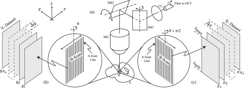
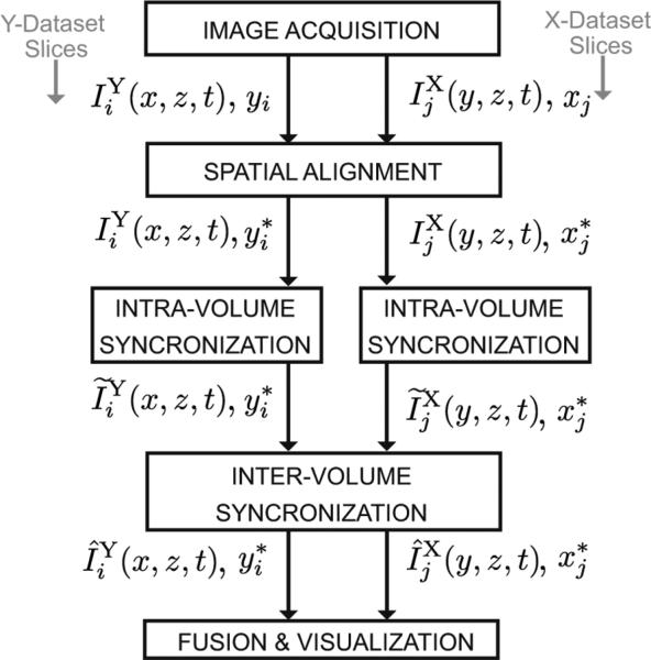
where y ∈ [y_min, y_max], z ∈[z_min, z_max], x_j = x₁ + (j – 1)Δ x, j = 1, 2, ... , N_x, x₁ is the initial x-position, Δx is the x-spacing, h^Y (x, y, z) is the PSF of the OCT system for this configuration, N_x is the number of X-slices acquired over times t ∈ [0, L), and $v_j^X$ are the temporal warping functions defined similarly to the $v_i^Y$. We note that the two PSFs, h^Y and h^X are related by a coordinate change, h^X (y, x, z) = h^Y (x, y, z). The OCT imaging setup is illustrated in Fig. 1. We note that the frame rate at which individual 2D sections can be acquired does not depend on their orientation. Specifically, the frame rate is the same whether the sections are oriented perpendicularly to the -x-or the y-axis. In the following text, we refer to ${\left\{I_i^Y\right\}}_{i=1,2,\dots ,N_y}^{}$ as the Y-dataset and ${\left\{I_j^X\right\}}_{j=1,2,\dots ,N_x}^{}$ as the X-dataset. The reconstruction problem is to estimate the inverse warping functions ${\left[v_i^Y\right]}^{-1}$ and ${\left[v_j^X\right]}^{-1}$ for each slice, so as to recover an estimate of I(x, y, z, t). The acquisition procedure above and the reconstruction steps below are summarized in Fig. 2.

Fig. 1.

OCT imaging setup. (a) x-y scanner allows recording vertical planes at arbitrary orientations around a vertical axis. The signal from the fiber of one arm of an OCT system is sent through an x-y scanner (consisting of two scanning mirrors SM1 and SM2) via a collimating lens (CL), into a microscope objective (MO) and to the heart (H) inside the sample (S). (b) Vertical sections (B-scans) are acquired by rapidly scanning along a fixed orientation θ. Each 2D OCT image frame along xz-plane (B-scan) is assembled from a collection of 1D signals (A-scans) that record the scattering within the sample along the vertical direction. The double arrow indicates the scanning motion produced by the galvanometer-mounted mirrors that can oscillate around a fixed axis. (c) Assembly of 2D OCT image frames along yz-plane with scanning orientation adjusted to θ + π/2.

Fig. 2.

Top-level block diagram showing the stages of the algorithm. The notation is explained in the text.

B. Spatial Alignment

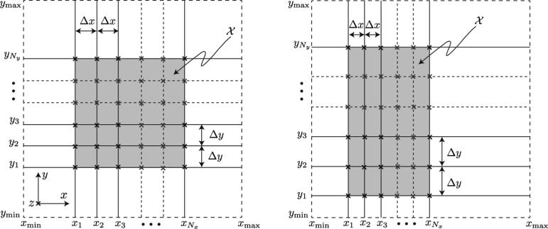
The above imaging geometry results in a set of xz-planes intersecting a set of yz-planes in lines that are parallel to the z-axis (Fig. 3). In our experimental OCT setup the orientations of the slices are known reliably (they are 90° apart), however, their positioning and spacings are not. Specifically, we assume that the parameters Θ = (x₁, y₁, Δx, Δy) are only known approximately and refine them using a method we will now describe.

Fig. 3.

Spatial organization of the slices in the X- and Y- datasets for two different values of Θ = (x₁, y₁, Δx, Δy), where the origin (x₁, y₁)and spacing between slices Δx and Δy are only known approximately in the two 3D+time datasets $I_i^Y$ and $I_j^X$. The z-axis is perpendicular to the viewing plane and is indicated with a cross. Y-dataset $I_i^Y$, i = 1, 2, ..., N_y spans [x_min, x_max] and X-dataset $I_j^X$, j = 1, 2, ..., N_x spans [y_min, y_max]. The slices from the two datasets intersect along lines parallel to z-axis (indicated with crosses). The shaded region indicates the domain $\mathcal{X}$.

First, to simplify the problem of spatially adjusting the positions of the slices, we convert our time-series in each section to a single image by averaging each sequence over one cardiac period

$${\stackrel{‒}{I}}_i^Y(x,z)=\frac{1}{T}{\int }_0^T{I}_i^Y(x,z,t)dt,i=1,2,\dots ,N_y$$

and

$${\stackrel{‒}{I}}_j^X(y,z)=\frac{1}{T}{\int }_0^T{I}_j^Y(y,z,t)dt,j=1,2,\dots ,N_x.$$ (5)

These images are time independent and do not depend on the fact that the sequences were acquired starting at arbitrary phases in the cardiac cycle. Note that the above average is computed only over t ∈ [0, T) and all frames corresponding to t > T are ignored. The period T can either be estimated visually (the algorithm only requires a rough estimate of the period to operate) or automatically computed using an algorithm we have previously described in [19]. For a given parameter vector Θ′ = (x′₁, y′₁, Δx′, Δy′), we then interpolate the slice-stacks as

$$\begin{array}{cc}\hfill {\stackrel{‒}{I}}^Y(x,y,z;{ϴ}^{\prime })& =\sum _{i=1}^{N_y}{\stackrel{‒}{I}}_i^Y(x,z){\phi }_{\mathrm{int}}^n\left(\frac{y-(y_1^{\prime }+(i-1)\Delta y^{\prime })}{{\Delta }_y}\right)\hfill \\ \hfill {\stackrel{‒}{I}}^X(x,y,z;{ϴ}^{\prime })& =\sum _{j=1}^{N_x}{\stackrel{‒}{I}}_j^X(y,z){\phi }_{\mathrm{int}}^n\left(\frac{x-(x_1^{\prime }+(j-1)\Delta x^{\prime })}{{\Delta }_x}\right)\hfill \end{array}$$ (6)

where ${\phi }_{\mathrm{Int}}^n$ are interpolating functions, e.g., cubic cardinal splines [23]. We estimate the optimal parameters Θ* = (x*₁, y*₁, Δx*, Δy*) by minimizing the mean absolute difference (MAD) between the interpolated datasets as

$${ϴ}^{\ast }\underset{{ϴ}^{\prime }}{\arg \min }\frac{1}{\mid \mathcal{X}\mid }{\int \int \int }_{\mathcal{X}}\mid {\stackrel{‒}{I}}^Y(x,y,z;{ϴ}^{\prime })-{\stackrel{‒}{I}}^X(x,y,z;{ϴ}^{\prime })\mid dxdydx$$ (7)

where $\mathcal{X}$ denotes the region over which the Y-and X-datasets overlap, see Fig. 3

$$\mathcal{X}=\{(x,y,z)\mid x\in [{\tilde{x}}_{\min },{\tilde{x}}_{\max }],y\in [{\tilde{y}}_{\min },{\tilde{y}}_{\max }],z\in [z_{\min },z_{\max }]\}$$ (8)

and $\mid \mathcal{X}\mid =({\tilde{x}}_{\max }-{\tilde{x}}_{\min })({\tilde{y}}_{\max }-{\tilde{y}}_{\min })(z_{\max }-z_{\min })$, with x̃_min = max(x_min, x′₁), x_max = min(x_max, x′_Nx) y_min = max(y_min, y′₁), y_max = min(y_max, y′_Ny).

$$\begin{array}{cc}\hfill {\tilde{x}}_{\min }& =\max (x_{\min },x_1^{\prime }),{\tilde{x}}_{\max }=\min (x_{\max },x_{N_x}^{\prime })\hfill \\ \hfill {\tilde{y}}_{\min }& =\max (y_{\min },y_1^{\prime }),{\tilde{y}}_{\max }=\min (y_{\max },y_{N_y}^{\prime }).\hfill \end{array}$$ (9)

C. Intra-Volume Synchronization

First, the slices in the Y-dataset are recursively synchronized to each other (without taking into account the slices in the X-dataset) using a technique previously described in [24]. Briefly, we determine the warping functions $w_i^Y$, that are estimates of the inverse warping functions ${\left[v_i^Y\right]}^{-1}\left(t\right)$, as the solutions to the minimization problem

$$w_i^Y=\arg \underset{w\in \mathcal{M}}{\min }\sum _{k\in {\mathcal{K}}_i}\left[(1-\lambda ){\int }_{x_{\min }}^{x_{\max }}{\int }_{z_{\min }}^{z_{\max }}{\int }_0^L\mid I_k^Y(x,z,w_k^Y\left(t\right))-I_i^Y(x,z,w\left(t\right))\mid dtdzdx+\lambda {\int }_0^L\mid \frac{d}{d}tw\left(t\right)-1\mid dt\right]$$ (10)

where ${\mathcal{K}}_i$ is the slice neighborhood of i such that any element k therein satisfies |i – k| ≤ 2, 0 < k < N_y, and $w_k^Y$ has been previously determined (we align each slice only to the already aligned slices in its neighborhood), 0 ≤ λ < 1, is the regularization parameter to favor either good matching between warped and reference sequences (λ = 0) or the temporal integrity of the warped sequence (λ → 1), and the set $\mathcal{M}$ is defined below. We initialize the algorithm with $w_{i_0}^Y\left(t\right)=t$, where i₀ is the reference slice. Subsequent warping functions $w_i^Y$ are determined by recursively aligning neighboring slices by first proceeding in increasing slice order of i = i₀ + 1, i₀ + 2, ..., N_y and then in decreasing slice order of i = i₀ – 1, i₀ – 2, ..., 1. In the minimization, we constrain the warping functions to be within the set of continuous, non-negative, and strictly increasing functions bounded by L, the length of the sequences, and defined over the interval [0, T), that is, $w_i\in \mathcal{M}:[0,T)\to [0,L)$, $t\mapsto w_i^Y\left(t\right)$, where $\mathcal{M}=\{w\in {\mathcal{C}}^1\left([0,T)\right)\mid 0\le w\left(t\right)<L$ and w(t₁)<w(t₂), t₁ < t₂}. To ensure that we can match at least one complete cardiac cycle that is in phase with the reference slice, our algorithm requires that $v_i^Y\left(L\right)-v_i^Y\left(0\right)>2T$.

In the most unfavorable case of temporal warping [see (3)], the heartbeat is slowed by a factor (1 + α) and the period lengthened accordingly to T_max = T(1 + α), leading to the requirement that the acquisition L length be at least L_min = 2T_max = 2(1 + α)Tto cover two periods. The minimization problem in (10) is solved efficiently in a dynamic programming framework in which we quantize the possible values of the warping function, making the problem equivalent to a lowest cost path search, whose solution we described previously in [5], [19], and [20]. Once the estimates $w_i^Y$ are determined, we define the warped Y-dataset as

$${\widehat{I}}_i^Y(x,z,t)=I_i^Y(x,z,w_i^Y\left(t\right)),t\in [0,T),i=1,2,\dots ,N_y.$$ (11)

Slices in the X-dataset are processed in a manner analogous to the Y-dataset to determine $w_j^X$, j = 1, 2, ..., N_x. However, we first ensure the reference slice (indexed by j₀) in the X-dataset matches the reference slice from the Y-dataset (indexed by i₀) as follows. The data along the line of intersection between the i₀th and the j₀th slices are extracted in the $I_{i_0}^Y$ and $I_{j_0}^X$ slice-sequences, as

$$L_{i_0,j_0}^Y(z,t)=I_{i_0}^Y(x_{j_0}^{\ast },z,t)$$

and

$$L_{i_0,j_0}^X(z,t)=I_{j_0}^X(y_{i_0}^{\ast },z,t)$$ (12)

respectively, where x*_j0 = x*₁ + (j₀ – 1)Δx* and y*_i0 = y*₁ + (i₀ – 1)Δy* are the slice positions determined in (7). The initial warping function for the X-dataset that matches $I_{j_0}^X$ to $I_{i_0}^Y$ is then found as

$$w_{j_0}^X=\arg \underset{w\in \mathcal{M}}{\min }\left[(1-\lambda ){\int }_{z_{\min }}^{z_{\max }}{\int }_0^L\mid L_{i_0,j_0}^Y(z,t)-L_{i_0,j_0}^X(z,w\left(t\right))\mid dtdz+\lambda {\int }_0^L\mid \frac{d}{dt}w\left(t\right)-1\mid dt\right]$$ (13)

which is a special case of the minimization in (10) and that we therefore solve using the same approach. Finally, after all $w_j^X$'s are determined by solving a problem similar to (10) for the X-dataset, we can define the warped X-dataset as

$${\tilde{I}}_j^X(y,z,t)=I_j^X(y,z,w_j^X\left(t\right))t\in [0,T),j=1,2,\dots ,N_x.$$ (14)

D. Inter-Volume Synchronization

For each slice in the Y-dataset, ${\tilde{I}}_i^Y$, we define the (theoretical) mean difference between the estimated inverse warping functions $w_i^Y$ to the true inverse function ${\left[v_i^Y\right]}^{-1}$ over all times t ∈ [0, T] as

$$d_i^Y=\underset{k\in \mathbb{Z}}{\min }\frac{1}{T}{\int }_0^T\mid w_i^Y\left(t\right)-{\left[v_i^Y\right]}^{-1}(t+kT)\mid dt.$$ (15)

This difference is defined as the minimum over all integers k to accommodate the underlying periodicity of the signal I(x, y, z, t), which leads to multiple possible solutions for $w_i^Y$ (the error is computed over the best acceptable solution). $d_i^Y$ corresponds to an average constant shift in time mismatch, which we empirically observed on simulated data (for which the true warping functions are known and $d_i^Y$ can be explicitly computed) to be nonzero on average and increasing for slices far away from the reference slice, due to error accumulation inherent to our recursive approach in synchronizing slice sequences (Fig. 5). To mitigate this error accumulation, we set out to find constant corrective terms ${\epsilon }_i^Y$, ${\epsilon }_j^X\in [0,T)$ that we use to correct the warping functions as

$${\tilde{w}}_i^Y\left(t\right)=w_i^Y\left({\mathcal{W}}_T(t+{\epsilon }_i^Y)\right)$$

and

$${\tilde{w}}_j^X\left(t\right)=w_j^X\left({\mathcal{W}}_T(t+{\epsilon }_j^X)\right)$$ (16)

where ${\mathcal{W}}_T:\mathbb{R}\to [0,T)$ denotes the wrapping operation

$${\mathcal{W}}_T\left(t\right)=t-\lfloor \frac{t}{T}\rfloor T$$ (17)

with ⌊ ⌋ the floor operation. The wrapping in the argument of the original estimate $w_i^Y$ and $w_j^X$ ensures that only available data at time-points in [0, L) are accessed. This corrective operation corresponds to circularly shifting the $w_i^Y$ -and $w_j^X$ -warped datasets in time by a constant.

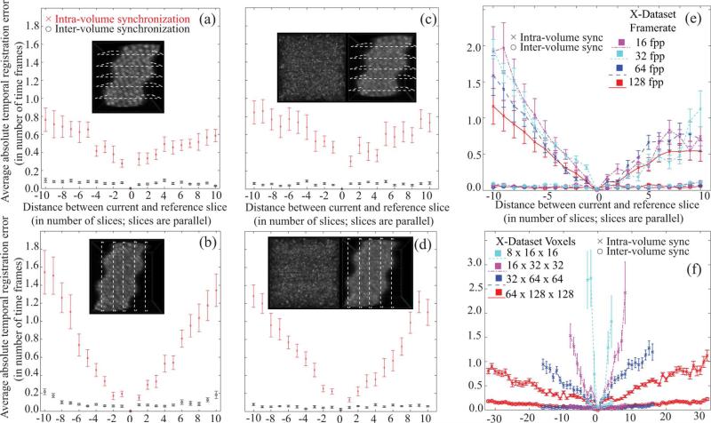
Fig. 5.

Temporal registration errors (TRE) accumulate with intra-volume synchronization at increasing distances from the reference slice. The proposed inter-volume synchronization limits the extent of these errors. (a) Y-dataset TREs, with inset showing a representative reference volume. (b) X-dataset TREs, inset shows reference volume. (c) TREs for Y-dataset with speckle multiplied, inset shows a speckle volume (left) and the generated reference volume with speckle (right). (d) TREs for X-dataset with speckle multiplied, inset shows a speckle volume (left) and the generated reference volume with speckle (right). (e) TREs for heart phantom X-dataset with fixed spatial resolution and varying temporal resolution measured in frames per period (fpp). (f) TREs for heart phantom X-dataset with fixed temporal resolution and varying spatial resolution sampled as N_x × N_y × N_x voxel dataset. In all plots, each point corresponds to the average absolute value of the registration error for one image sequence, obtained by averaging the absolute errors over all the time points. Error bars correspond to standard deviation over 100 simulations, divided by $\sqrt{100}$. For (a) and (c) Y-dataset was of 41 × 21 × 41 voxels at 19 fpp, for (b) and (d) X-dataset was of 21 × 41 × 41 voxels at 19 fpp, for (e) X-dataset was of 21 × 41 × 41 voxels, and for (f) X-dataset had temporal resolution of 19 fpp. (Color Online)

We use the fact that the time-signals at the intersections between the slices in the Y-and X-datasets match-up in order to estimate the corrective terms ${∊}_i^Y$ and ${∊}_j^X$ for the Y-and X-datasets, respectively. Using the starting slice location and slice-spacing determined in the spatial alignment step, the data on the line of intersection between the ith and the jth slice are extracted as

$$L_{i,j}^Y(z,t)={\tilde{I}}_i^Y((x_1^{\ast }+(j-1)\Delta x^{\ast }),z,t)$$

and

$$L_{i,j}^X(z,t)={\tilde{I}}_j^X((y_1^{\ast }+(i-1)\Delta y^{\ast }),z,t).$$ (18)

The data in the Y-and X-datasets on these intersecting lines parallel to the z-axis are compared using the cost function

$$Q_{i,j}\left(s\right)={\int }_z{\int }_0^T{\mid L_{i,j}^X(z,t)-L_{i,j}^Y(z,{\mathcal{W}}_T(t-s))\mid }^{2}dtdz$$ (19)

where $s\in \mathbb{R}$ is a constant shift in time. The relative shift s_j,j between slice ${\tilde{I}}_i^Y$ and slice ${\tilde{I}}_j^X$ is determined by minimizing the above cost function to find the best shift

$$s_{i.j}=\underset{s\in [0,T)}{\arg \min }{Q}_{i,j}\left(s\right)$$ (20)

by correlating the two signals [19]. We then determine the absolute shifts ${\epsilon }^Y={[{\epsilon }_1^Y,{\epsilon }_2^Y,\dots ,{\epsilon }_{N_y}^Y]}^T$ and ${\epsilon }^X={[{\epsilon }_1^X,{\epsilon }_2^X,\dots ,{\epsilon }_{N_x}^X]}^T$ by considering their relation to the above determined relative shifts s_i,j

$$s_{i,j}={\mathcal{W}}_T({\epsilon }_i^Y-{\epsilon }_j^X),\text{with}i=1,2,\dots N_y$$

and

$$j=1,2,\dots ,N_x.$$ (21)

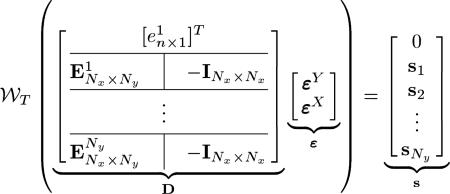
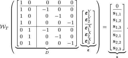
For N_y slices in the Y-dataset intersecting the N_x slices in the X-dataset, we rewrite (21) in matrix form as

(22)

where matrix D is of size m × n, with m = N_xN_y +1 and n = N_x + N_y, vector ε has n elements, vector has m elements, ${\mathcal{W}}_T\left(\mathbf{M}\right)$ is the element-wise wrapping operation on the matrix M, $e_{n\times 1}^i={[\dots ,0,1,0,\dots ]}_{n\times 1}^T$ is an n-element column vector with the ith element being 1 and all other elements being zero and ${\mathbf{E}}_{m\times n}^i={[\dots ,0_{n\times 1},1_{n\times 1},0_{n\times 1},\dots ]}_{m\times n}$ an n-column matrix with its ith column being $1_{n\times 1}={[1,1,\dots ,1]}^T$, an n-element column vector with all elements being 1, and all other columns being $0_{n\times 1}={[0,0,\dots ,0]}^T$, an n-element column vector with all zeros, –I is a N_x × N_x negative identity matrix, and s_i = [s_i,1, s_i,2, ..., s_i, N_x]^T. For example, for a system with N_y = 2 and N_x = 3 (22) would be

(23)

Given that the ${\epsilon }_i^Y$ and ${\epsilon }_j^X$ are in [0, T), their differences are confined to (–T, T) and we can rewrite the wrapping operation in (22) as

$$\mathbf{D}\epsilon =\mathbf{s}-\mathbf{k}T$$ (24)

with K ∈ {0, 1}^m (that is, each of the m elements of vector k can be either 0 or 1). We further recast (24) into the matrix form

$$\underset{\mathbf{A}}{\underbrace{\left[\mathbf{D}\mathbf{I}\right]}}\underset{\mathbf{x}}{\underbrace{\left[\begin{array}{c}\hfill {\epsilon }^{\prime }\hfill \\ \hfill \mathbf{k}\hfill \end{array}\right]}}=\underset{\mathbf{b}}{\underbrace{{\mathbf{s}}^{\prime }}}$$ (25)

where I is an identity matrix of size m × m, A is of size m × (n + m), X is of size (n + m) × 1, b is of size m × 1, ε′ = ε/T and s′ = s/T. This problem usually has no exact solution since the measured relative shifts in are themselves estimates. Our strategy is therefore to seek an approximate solution to this problem in the ${\ell }_1$-sense, i.e.,

$$\widehat{x}=\underset{\mathbf{x}}{\arg \min }\Vert Ax-\mathbf{b}\Vert$$ (26)

which is equivalent to the minimization problem

$$\widehat{x}=\underset{\mathbf{x},\mathbf{y}}{\arg \min }\sum _{i=1}^m{y}_i\mathrm{s}.\mathrm{t}-\mathbf{y}\le \mathbf{Ax}-\mathbf{b}\le \mathbf{y}{\varnothing }_{(n+m)\times 1}\le \mathbf{x}\le 1_{(n+m)\times 1}$$ (27)

with the lower m elements of x (corresponding to k) being binary integers, $0_{p\times 1}$ a vector with p zeros and $1_{p\times 1}$ a vector with all its p elements being 1. The above problem is a mixed integer linear programming (MILP) problem and can be rewritten as

$$\widehat{\mathit{x}}=\underset{\tilde{\mathbf{x}}}{\arg \min }{\tilde{\mathit{c}}}^T\tilde{\mathit{x}},\mathrm{s}.\mathrm{t}\tilde{\mathit{A}}\tilde{x}\le \tilde{b}\tilde{\mathit{x}}=\left[\begin{array}{c}{\mathbf{x}}_{(n+m)\times 1}\hfill \\ {\mathbf{y}}_{m\times 1}\hfill \end{array}\right],$$ (28)

$$\tilde{\mathit{c}}=\left[\begin{array}{c}{0}_{(n+m)\times 1}\hfill \\ 1_{m\times 1}\hfill \end{array}\right]0_{(n+2m)\times 1}\le \tilde{\mathit{x}}\le 1_{(n+2m)\times 1}$$

$$\tilde{\mathit{A}}=\left[\begin{array}{cc}\hfill {\mathbf{A}}_{m\times (n+m)}\hfill & \hfill -{\mathbf{I}}_{m\times m}\hfill \\ \hfill -{\mathbf{A}}_{m\times (n+m)}\hfill & \hfill -{\mathbf{I}}_{m\times m}\hfill \end{array}\right]\tilde{\mathit{b}}=\left[\begin{array}{c}{\mathbf{b}}_{m\times 1}\hfill \\ -{\mathbf{b}}_{m\times 1}\hfill \end{array}\right]$$

where the subscripts indicate the size of the matrices. The absolute shifts are confined to the real interval [0, T] and are given by $\widehat{\epsilon }={\widehat{\epsilon }}^{\prime }T$, where ${\widehat{\epsilon }}^{\prime }$ corresponds to the first n elements of x̂, while the binary integers k are the next m elements. Equation (28) has the form of a generic minimization problem that can be solved efficiently using state-of-the-art optimization packages, such as the CPLEX Optimization Studio software [25]. The corrective shifts $\widehat{\epsilon }$ are then applied to the slices in the Y-and X-datasets to get

$${\widehat{I}}_i^Y(x,z,t)={\tilde{I}}_i^Y(x,z,{\mathcal{W}}_T(t-{\widehat{\epsilon }}_i^Y))$$

and

$$\begin{array}{cc}\hfill {\widehat{I}}_j^X(y,z,t)=& {\tilde{I}}_j^X(y,z,{\mathcal{W}}_T(t-{\widehat{\epsilon }}_j^X)),t\in [0,T)\hfill \\ \hfill i=& 1,2,\dots ,N_y,j=1,2,\dots ,N_x.\hfill \end{array}$$ (29)

Finally, the two resulting datasets are spatially interpolated and fused (by averaging pixels across the datasets in regions of overlap), to get a single 3D+time reconstruction of the heart.

III. EXPERIMENTS AND RESULTS

A. Synthetic Dataset

We evaluated the reconstruction accuracy of the proposed method using a previously described synthetic heart tube phantom [19], that is briefly presented here. A parametric, analytic equation describes the intensity of the static tube at a given point (x, y, z) in 3D space. Evaluating this parametric equation at different spatial coordinates gives the complete static heart-tube phantom. For deforming this heart-tube periodically, the spatial coordinates are subjected to an affine transform defined by a matrix whose coefficients are a weighted sum of sinusoidal and cosinusoidal functions at harmonic frequencies. The data acquisition on this periodically deforming heart-tube phantom is then simulated by evaluating the phantom values sequentially for different Y-slices to get a synthetic Y-dataset [$I_i^Y$, (2)] and for different X-slices to get a synthetic X-dataset [$I_j^X$, (4)]. A different random time shift drawn from a uniform distribution of $\mathcal{U}(-T,T)$ is used to generate a linear warping function (time-offset) for each acquired image sequence, similar to the approach in [19]. The spatial resolution of the heart tube phantom Y-dataset was N_x × N_y × N_z = 41 × 21 × 41 voxels and that of X-dataset was 21 × 41 × 41 voxels. The temporal resolution of both datasets was 19 frames per period (fpp) and each of the slice sequences was of length L = 40 frames.

We reconstructed the simulated heart tube phantom data using our proposed method. The reconstructed volumes and absolute difference with the ground truth phantom are shown after we independently synchronized the Y-and X-datasets [Fig. 4(d)–(g)] and after we jointly synchronized the Y-and X-datasets using our proposed technique [Fig. 4(h)–(k)]. Using only a single orientation to synchronize the slices leads to increased error accumulation for slices at increasing distance from the reference slice [Fig. 4(f) and (g)]. Conversely, when the slices from both orientations are co-registered simultaneously, error accumulation is mitigated [Fig. 4(j) and (k)].

Fig. 4.

Still image of a synthetic heart phantom. (a) Reference phantom. (b) and (c) Sequentially acquired slices of Y- and X-datasets, respectively. (d) Y-dataset after independent intra-volume synchronization. Dotted line in (b) indicates the reference slice used for synchronization. (e) X-dataset after independent intra-volume synchronization. Dotted line in (c) indicates the reference slice used for synchronization. (f) Absolute difference between frames in (d) and (a). (g) Absolute difference between frames in (e) and (a). (h) and (i) Y- and X-datasets, respectively, after inter-volume synchronization. (j) Absolute difference between frames in (h) and (a). (k) Absolute difference between frames in (i) and (a). Also see Movies 1 and 2 in the supplementary files.

We quantified the accuracy of our approach as follows. The weights of the sine and cosine functions in the affine transform were selected randomly (from a zero mean normal distribution with σ = 0.1) up to the third harmonic (higher harmonics were set to zero) to generate 100 dynamic reference phantoms as well as corresponding sequential parallel slice measurements (Y-and X-datasets) with acquisition starting at random time-shifts (drawn from $\mathcal{U}(-T,T)$) for each slice-sequence. We then reconstructed the two datasets in each of the above 100 simulations and compared the ground-truth shifts with the corresponding reconstruction shifts of every slice before and after inter-volume synchronization (specifically, the error in the estimated time-offset was computed by comparing the ground truth time offset with the constant component of the estimated warping function). The mean error between estimated and ground truth time-offset [Fig. 5(a) and (b)] indicate that the inter-volume synchronization of the slices mitigates the registration error accumulated during the recursive inter-volume synchronization of the slices. The gain is particularly important for slices that are furthest from the reference slice.

In order to investigate the sensitivity of our method to speckle, we generated dynamic time-evolving (nonstationary) speckle volumes that emulated the speckle observed during OCT imaging [26] with identical sampling as in the simulations above. We scaled the speckle intensities to the interval [0, 1, 0.9] and multiplied the speckle volumes voxel-by-voxel with the dynamic heart phantoms, to generate the phantom datasets with speckle [see insets in Fig. 5(c) and (d)]. We then repeated the reconstruction experiment with the datasets containing speckle. Fig. 5(c) and (d) shows that our reconstruction method performed similarly well in this case as in the speckle-free simulation. This robustness is likely due to the fact that our algorithm solves the registration problem over the entire dataset, globally, limiting the influence of local intensity changes.

We further investigated the influence of temporal sampling on the performance of our algorithm. We generated a series of dynamic heart phantoms for a given spatial resolution and cardiac period but captured at different frame-rates (16, 32, 64, and 128 fpp). Again we gathered reconstruction results over 100 simulations. The registration errors after independent intra-volume synchronization increased when the number of frames per period decreased. The inter-volume synchronization successfully compensated for the accumulated registration errors in all tested temporal samplings [Fig. 5(e)].

Finally, we investigated the influence of spatial sampling on the reconstruction accuracy. The dynamic heart phantom was sampled at spatial resolution of N_x × N_y × N_z voxels and temporal resolution of 19 fpp. The N_x, N_y, and N_z values were varied to simulate changing spatial resolution, and in each case the registration results were plotted over 100 simulations. The registration error after independent intra-volume synchronization phase increased with the coarser sampling of the phantom. However, as seen in Fig. 5(f), the inter-volume synchronization step was able to overcome these registration errors further demonstrating the effectiveness of our algorithm in reconstructing 4D volumes.

B. Experimental OCT Dataset

To evaluate the feasibility of our method in practice, we acquired image sequences of a live E9.5 mouse and an E10.5 rat embryo using a swept-source OCT (SS-OCT) system as previously described by Larina et al. [27]. Briefly, the experimental system was customized from a Thorlabs SL1325-P16 system which utilizes a broadband swept-source laser with a central wavelength of λ₀ = 1325 nm, a bandwidth of Δλ = 110 nm, an output power P = 12 mW, and an A-line scanning frequency of 16 kHz [leading to an effective frame rate of 51 2D frames per second (fps)].

We sequentially acquired two perpendicular OCT data sets from the beating heart of an E9.5 mouse and E10.5 rat embryos. The embryos were cultured on the imaging stage according to previously described protocols [3], [4]. The OCT datasets were acquired with 10 μm steps between sections.

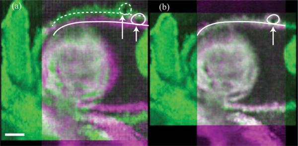
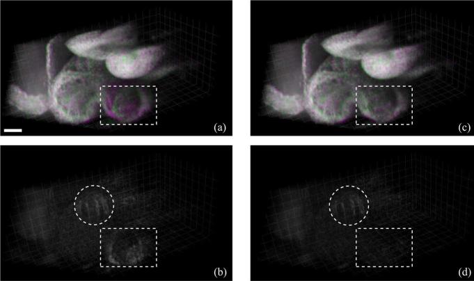
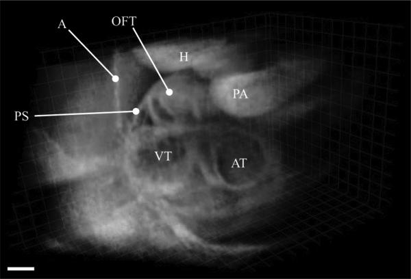
In the E9.5 mouse dataset, each of the N_y = 63 slice-sequences in the Y-dataset and N_x = 78 slice-sequences in the X-dataset consisted of 150 frames of 256 × 512 pixels (256 A-scans, each with 512 pixels) acquired at 51 fps. We implemented our algorithm in MATLAB R2011b. The algorithm required about 10 h for reconstructing the OCT dataset [containing two volumes of 256 × 256 × 512 × 30 voxels each (T = 30) or about 8.5 GB in total starting from the two datasets of size 256 × 63 × 512 × 150 and 78 × 256 × 512 × 150 voxels or about 11 GB in total)] on a Windows 64-bit machine, equipped with a dual-core Intel Xeon 3.4 GHz CPU and 16 GB RAM. Specifically, the spatial alignment step using MATLAB's fminsearch routine took 1 h, the intra-volume synchronization step took 3.5 h, the inter-volume synchronization step took 1.5 h (with the MILP optimization needing 30 min) and the final interpolation and fusion step took 4 h. The resulting dataset was visualized using Bitplane Imaris software. The OCT system hardware provided an initial estimate Θ = (–0.62 mm, –0.54 mm, +0.01 mm, +0.01 mm) that our algorithm refined to Θ* = (–0.583 mm, –0.457 mm, +0.008 mm, +0.008 mm). Visual inspection of the reconstructed dynamic volumes (Fig. 6 and Movie 3 in the supplementary file) shows the improvement in the match between the two sets when using Θ*. Fig. 7 and Movie 4 (see supplementary file) show the results after intra-volume and inter-volume synchronization of the OCT dataset. Since a successful synchronization of the X-and Y-datasets should result in two identical (up to the effect of the nonisotropic PSF) datasets, our approach allows directly visualizing the quality gained over using only a single dataset directly: any discrepancy is visible in the difference image and could therefore be used as a local map of reconstruction confidence. This could, for example, be useful to identify regions where the heart does not conform to the quasi-periodicity assumptions. Fig. 7(d) illustrates the improved alignment between the XY-datasets after inter-volume synchronization. Finally, the fused volume is shown in Fig. 8.

Fig. 6.

xy-section from the time-averaged experimental OCT Y- and X-datasets at z = 211, false-colored magenta and green, respectively. (a) Misalignment (along the solid and dashed curves) between the datasets when they are interpolated using Θ. (b) Datasets show good spatial alignment (along the solid curve) after they are interpolated using the refined Θ*. Scale bar is 100 μm. Also see Movie 3 in the supplementary file. (Color Online).

Fig. 7.

Synchronization results on experimental OCT dataset at time t = 252 ms. (a) Dual-channel volumetric dataset containing Y-dataset (false-colored magenta) and X-dataset (false-colored green) after independent intra-volume synchronization. When the XY-datasets are in-sync their colors add up to produce gray. (b) Absolute difference between the X- and Y-datasets with slices in X-and Y-volumes synchronized independently. (c) XY-datasets after inter-volume synchronization. (d) Absolute difference between the X- and Y-datasets after inter-volume synchronization. The dotted rectangles show areas that exhibit improved alignment after inter-volume synchronization. The dotted circles indicate areas near the outflow tract where the Y- and X-datasets are mismatched due to sample movement between their respective acquisition. Scale bar is 100 μm. Also see Movie 4 in the supplementary file. (Color online)

Fig. 8.

3D-visualization of the reconstructed and fused experimental OCT dataset from a E9.5 mouse embryo showing different cardiac structures. PS: pericardial sac; A: Amnion; OFT: Outflow tract; H: Head; PA: Pharyngial arch; AT: Atrium; and VT: Ventricle are marked. Scale bar is 100 μm. Also see Movie 5 in the supplementary file.

In the E10.5 rat dataset, the Y-dataset consisted of N_y=63 slice-sequences and the X-dataset of N_x = 56 slice-sequences, with each sequence consisting of 400 frames of 128 × 512 pixels acquired at 91 fps (T = 72). The OCT system hardware produced Θ = (–0.30 mm, –0.61 mm, +0.01 mm, +0.01 mm) which our spatial alignment refined to Θ* = (–0.291 mm, –0.603 mm, +0.008 mm, +0.008 mm). We also acquired a dataset in the STAR geometry [21] which consisted of 60 image sequences, each with 400 frames of 128 × 512 pixels acquired at 91 fps. The angle between the neighboring sequences was set to 3° and the axis of imaging plane rotation (central line) was positioned over the highly moving structure to ensure good reference signal for synchronization. The acquired Y-and X-datasets were recontructed using the proposed method and the STAR dataset was reconstructed following Larina et al. [21]. Fig. 9(a) and (b) shows that our method improves on previous single parallel dataset reconstructions. While both the STAR and our proposed method produce reconstructions that are less prone to error accumulation, Fig. 9(b) and (c) shows that our proposed method has isotropic resolution unlike the STAR method, whose resolution decreases away from the center due to the cylindrical sampling geometry.

Fig. 9.

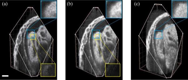
Comparison of reconstructions of a E10.5 rat embryo heart using different techniques. (a) Reconstruction using only one set of parallel slices (Y-dataset after intra-volume synchronization). The lower inset shows a residual difference between (a) and the (self-validating) fused dataset obtained in (b). (b) Fused dataset obtained using two orthogonal sets of parallel slices (proposed method). The lower inset shows the difference in the boxed region between the (matching) inter-volume synchronized Y- and X-datasets. (c) Reconstruction using STAR method [21]. The upper insets show the isotropic resolution produced by parallel slice based methods [(a), (b)] while the cylindrical geometry is visible in the STAR method (c). Scale bar is 100 μm. (Color Online).

To verify that our method was not sensitive to the precise choice of reference slices used to initialize the reconstruction, we kept the Y-dataset reference slice fixed at the middle slice $I_{j_0}^Y$, j₀ = 32 and reconstructed the volumes for five different choices of the X-dataset reference slice $I_{i_0}^X$, which resulted in similar reconstructions each time (Fig. 10).

Fig. 10.

Reconstruction results for the E10.5 rat embryo dataset with N_y = 63 slices and N_x = 56 slices. Different reference slices, $I_{j_0}^X$, were chosen in the X-dataset while keeping the reference slice for the Y-dataset, $I_{i_0}^Y$, fixed at the middle slice (i₀ = 32) for the reconstructions. (a)–(e) Stills from the volumes obtained after only intra-volume synchronization. The circle indicates regions with misalignment between the X-and Y-datasets. (f)–(j) Corresponding stills from volumes obtained after inter-volume synchronization. The circles mark region that show improved alignment between the X-and Y-datasets. (a) and (f) j₀ = 3; (b) and (g) j₀ = 17; (c) and (h) j₀ = 28; (d) and (i) j₀ = 40; and (e) and (f) j₀ = 54. The locations of the reference slices in each dataset are indicated by the dashed planes. Scale bar is 100 μm. (Color Online).

IV. DISCUSSION

Methods for 4D reconstruction that only use one set of parallel slice-sequences and recursively register the neighboring slices starting from a reference slice lead to error accumulation that can be most severe for slices that are furthest from the reference. One way to correct these errors is to use the information from an additional orthogonal plane acquired to intersect all the other parallel planes [7]. However, the position of the orthogonal plane needs to be manually chosen so as to contain the beating heart in all the intersecting lines. A second way to avoid these registration errors is to acquire the slice-sequences in a star-geometry so that the sections intersect along one common line and temporally register them based on data on this line [21], [22]. However, this results in variable resolution due to the required transformation from cylindrical to Cartesian geometry. Our proposed technique takes advantage of the multi-view geometry to synchronize slices and mitigates the registration errors while not depending on the sole manual selection of an orthogonal slice position and while ensuring homogenous resolution of the reconstructed, fused volume. It is also self-validating, since whenever the two reconstructed datasets coincide, one can be confident that the true object has been recovered (Fig. 7(d) and Movie 4 in the supplementary file).

Considerable gains in computation time could likely be obtained by employing faster interpolation routines, parallel processor cores and GPUs. The algorithm could further benefit from the use of fast solid-state hard drives for data storage and retrieval.

Some of the shortcomings or our algorithm are discussed below. The spatial alignment step of our algorithm registers the two datasets by translation and scaling in the xy-plane only. In particular, any global sample drifts or rotation that occur over the acquisition of the sample are not compensated for by our method. In our experimental dataset, such a spatial change appears to occur in one region of the heart, the outflow tract, where the spatial registration, a global, homogeneous transform, does not correct for the local spatial dissimilarities. (Fig. 7 dotted circles). Finally, though our approach does not require any manual selection of a specific orthogonal slice for correction, it requires one to choose the reference slices in the two datasets [ and in (13)] in such a manner that they intersect the beating heart. Typically in our imaging geometry it is straightforward to make this choice, since there exist many such pairs of slice-sequences intersecting within the beating heart.

V. CONCLUSION

We have presented a technique for reconstruction of an 3D+time cardiac dataset from two orthogonal sets of nongated OCT slice-sequences. We validated the technique using a synthetically generated dynamic heart-tube phantom and characterized its effectiveness in reducing the errors accumulated during temporal registration of the slice-sequences separately in each perpendicular dataset. We demonstrated the applicability of our technique in practice by reconstructing a 3D+time cardiac volume of E9.5 mouse and E10.5 rat embryos. We expect our approach to be particularly relevant for the morphological and functional cardiac analysis in embryos.

References

- 1.Yelbuz T, Choma M, Thrane L, Kirby M, Izatt J. A new high-resolution imaging technology to study cardiac development in chick embryos. Circulation. 2002;106:2771–2774. doi: 10.1161/01.cir.0000042672.51054.7b. [DOI] [PubMed] [Google Scholar]
- 2.Larina I, Larin K, Justice M, Dickinson M. Optical coherence tomography for live imaging of mammalian development. Curr. Opin. Genet. Dev. 21:579–584. doi: 10.1016/j.gde.2011.09.004. [DOI] [PMC free article] [PubMed] [Google Scholar]
- 3.Larina I, Sudheendran N, Ghosn M, Jiang J, Cable A, Larin K, Dickinson M. Live imaging of blood flow in mammalian embryos using Doppler swept-source optical coherence tomography. J. Biomed. Opt. 2008;13(1–3):060506–1–060506-3. doi: 10.1117/1.3046716. [DOI] [PubMed] [Google Scholar]
- 4.Larina I, Ivers S, Syed S, Dickinson M, Larin K. Hemodynamic measurements from individual blood cells in early mammalian embryos with Doppler swept source OCT. Opt. Lett. 2009;34:986–988. doi: 10.1364/ol.34.000986. [DOI] [PMC free article] [PubMed] [Google Scholar]
- 5.Larin KV, Larina IV, Liebling M, Dickinson ME. Live imaging of early developmental processes in mammalian embryos with optical coherence tomography. J. Innov. Opt. Health Sci. 2009 Jan.2(3):253–259. doi: 10.1142/S1793545809000619. [DOI] [PMC free article] [PubMed] [Google Scholar]
- 6.Gargesha M, Jenkins M, Wilson D, Rollins A. High temporal resolution OCT using image-based retrospective gating. Opt. Exp. 2009;17:10786–10799. doi: 10.1364/oe.17.010786. [DOI] [PMC free article] [PubMed] [Google Scholar]
- 7.Liu A, Wang R, Thornburg KL, Rugonyi S. Efficient postacquisition synchronization of 4-D nongated cardiac images obtained from optical coherence tomography: Application to 4-D reconstruction of the chick embryonic heart. J. Biomed. Opt. 2009 Jan.14(4):044020–1–044020-11. doi: 10.1117/1.3184462. [DOI] [PubMed] [Google Scholar]
- 8.Skare S, Andersson JLR. On the effects of gating in diffusion imaging of the brain using single shot EPI. Magn. Reson. Imag. 2001 Oct.19(8):1125–1128. doi: 10.1016/s0730-725x(01)00415-5. [DOI] [PubMed] [Google Scholar]
- 9.Kachelrieß M, Sennst DA, Maxlmoser W, Kalender WA. Kymogram detection and kymogram-correlated image reconstruction from subsecond spiral computed tomography scans of the heart. Med. Phys. 2002 Jul.29(7):1489–1503. doi: 10.1118/1.1487861. [DOI] [PubMed] [Google Scholar]
- 10.Markl M, Chan FP, Alley MT, Wedding KL, Draney MT, Elkins CJ, Parker DW, Wicker R, Taylor CA, Herfkens RJ, Pelc NJ. Time-resolved three-dimensional phase-contrast MRI. J. Magn. Reson. Imaging. 2003 Apr.17(4):499–506. doi: 10.1002/jmri.10272. [DOI] [PubMed] [Google Scholar]
- 11.Jerecic R, Bock M, Nielles-Vallespin S, Wacker C, Bauer W, Schad LR. ECG-gated Na-23-MRI of the human heart using a 3D-radial projection technique with ultra-short echo times. Magn. Reson. Mater. Phys., Biol., Med. 2004 May;16(6):297–302. doi: 10.1007/s10334-004-0038-8. [DOI] [PubMed] [Google Scholar]
- 12.Taylor JM, Saunter CD, Love GD, Girkin JM, Henderson DJ, Chaudhry B. Real-time optical gating for three-dimensional beating heart imaging. J. Biomed. Opt. 2011;16(11):116021–1–116021-8. doi: 10.1117/1.3652892. [DOI] [PubMed] [Google Scholar]
- 13.Bartling SH, Kuntz J, Semmler W. Gating in small-animal cardio-thoracic CT. Methods. 2010;50(1):42–49. doi: 10.1016/j.ymeth.2009.07.006. [DOI] [PubMed] [Google Scholar]
- 14.Dinkel J, Bartling SH, Kuntz J, Grasruck M, Kopp-Schneider A, Iwasaki M, Dimmeler S, Gupta R, Semmler W, Kauczor H-U, Kiessling F. Intrinsic gating for small-animal computed tomography a robust ECG-less paradigm for deriving cardiac phase information and functional imaging. Circulat., Cardiovasc. Imag. 2008 Jan.1(3):235–243. doi: 10.1161/CIRCIMAGING.108.784702. [DOI] [PubMed] [Google Scholar]
- 15.Ertel D, Pflederer T, Achenbach S, Kachelrieß M, Steffen P, Kalender WA. Validation of a raw data-based synchronization signal (kymogram) for phase-correlated cardiac image reconstruction. Eur. Radiol. 2008 Feb.18(2):253–262. doi: 10.1007/s00330-007-0752-5. [DOI] [PubMed] [Google Scholar]
- 16.Jenkins M, Rothenberg F, Roy D, Nikolski V, Hu Z, Watanabe M, Wilson D, Efimov I, Rollins A. 4D embryonic cardiography using gated optical coherence tomography. Opt. Exp. 2006 Jan.14(2):736–748. doi: 10.1364/opex.14.000736. [DOI] [PubMed] [Google Scholar]
- 17.Jenkins MW, Chughtai OQ, Basavanhally AN, Watanabe M, Rollins AM. In vivo imaging of the embryonic heart using gated optical coherence tomography. J. Biomed. Opt. 2007 May;12(03):030505–030505. doi: 10.1117/1.2747208. [DOI] [PubMed] [Google Scholar]
- 18.Mariampillai A, Standish BA, Munce NR, Randall C, Liu G, Jiang JY, Cable AE, Vitkin IA, Yang VXD. Doppler optical cardiogram gated 2D color flow imaging at 1000 fps and 4D in vivo visualization of embryonic heart at 45 fps on a swept source OCT system. Opt. Exp. 2007 Jan.15(4):1627–1–1638-3. doi: 10.1364/oe.15.001627. [DOI] [PubMed] [Google Scholar]
- 19.Liebling M, Forouhar A, Gharib M, Fraser S, Dickinson M. Four-dimensional cardiac imaging in living embryos via postacquisition synchronization of nongated slice sequences. J. Biomed. Opt. 2005 Sep-Oct;10(5):054001–1–054001-10. doi: 10.1117/1.2061567. [DOI] [PubMed] [Google Scholar]
- 20.Liebling M, Forouhar A, Wolleschensky R, Zimmerman B, Ankerhold R, Fraser S, Gharib M, Dickinson M. Rapid three-dimensional imaging and analysis of the beating embryonic heart reveals functional changes during development. 235. Dev. Dynam. 2006 Nov.(11):2940–2948. doi: 10.1002/dvdy.20926. [DOI] [PubMed] [Google Scholar]
- 21.Larina IV, Larin KV, Dickinson ME, Liebling M. Sequential turning acquisition and reconstruction (STAR) method for four-dimensional imaging of cyclically moving structures. Biomed. Opt. Exp. 2012 Mar.3(3):650–660. doi: 10.1364/BOE.3.000650. [DOI] [PMC free article] [PubMed] [Google Scholar]
- 22.Happel C, Thommes J, Thrane L, Maenner J, Ortmaier T, Heimann B, Yelbuz T. Rotationally acquired four-dimensional optical coherence tomography of embryonic chick hearts using retrospective gating on the common central a-scan. J. Biomed. Opt. 2011 Sep.16(9):096007–1–096007-3. doi: 10.1117/1.3622491. [DOI] [PMC free article] [PubMed] [Google Scholar]
- 23.Thévenaz P, Blu T, Unser M. Interpolation revisited. IEEE Trans. Med. Imag. 2000 Jul.19(7):739–758. doi: 10.1109/42.875199. [DOI] [PubMed] [Google Scholar]
- 24.Liebling M, Vermot J, Forouhar A, Gharib M, Dickinson M, Fraser S. Nonuniform temporal alignment of slice sequences for four-dimensional imaging of cyclically deforming embryonic structures. Proc. ISBI 2006. 2006 Apr.:1156–1159. [Google Scholar]
- 25.IBM ILOG CPLEX Optimization Studio 2012 [Online]. Available: http://www-01.ibm.com/software/integration/optimization/cplex-optimization-studio/ [Google Scholar]
- 26.Duncan DD, Kirkpatrick SJ. The copula: A tool for simulating speckle dynamics. J. Opt. Soc. Am. A. 2008 Jan.25(1):231–237. doi: 10.1364/josaa.25.000231. [DOI] [PubMed] [Google Scholar]
- 27.Larina IV, Furushima K, Dickinson ME, Behringer RR, Larin KV. Live imaging of rat embryos with Doppler swept-source optical coherence tomography. 14. J. Biomed. Opt. 2009;(5):050506–050506. doi: 10.1117/1.3241044. [DOI] [PMC free article] [PubMed] [Google Scholar]
Associated Data
This section collects any data citations, data availability statements, or supplementary materials included in this article.