Exploration of scanning effects in multi-site structural MRI studies

Abstract

Background

Pooling of multi-site MRI data is often necessary when a large cohort is desired. However, different scanning platforms can introduce systematic differences which confound true effects of interest. One may reduce multi-site bias by calibrating pivotal scanning parameters, or include them as covariates to improve the data integrity.

New method

In the present study we use a source-based morphometry (SBM) model to explore scanning effects in multi-site sMRI studies and develop a data-driven correction. Specifically, independent components are extracted from the data and investigated for associations with scanning parameters to assess the influence. The identified scanning-related components can be eliminated from the original data for correction.

Results

A small set of SBM components captured most of the variance associated with the scanning differences. In a dataset of 1460 healthy subjects, pronounced and independent scanning effects were observed in brainstem and thalamus, associated with magnetic field strength-inversion time and RF-receiving coil. A second study with 110 schizophrenia patients and 124 healthy controls demonstrated that scanning effects can be effectively corrected with the SBM approach.

Comparison with existing method(s)

Both SBM and GLM correction appeared to effectively eliminate the scanning effects. Meanwhile, the SBM-corrected data yielded a more significant patient versus control group difference and less questionable findings.

Conclusions

It is important to calibrate scanning settings and completely examine individual parameters for the control of confounding effects in multi-site sMRI studies. Both GLM and SBM correction can reduce scanning effects, though SBM’s data-driven nature provides additional flexibility and is better able to handle collinear effects.

1. Introduction

Structural magnetic resonance imaging (sMRI) is increasingly used to study the morphology of the living brain given its non-invasive nature. Based on high resolution T₁-weighted images, measures can be derived to quantify brain structure for further analysis such as assessment of neurological diseases (Fornito et al., 2009; Glahn et al., 2008). A variety of computational methods have been developed to deal with the anatomical complexity, one of those commonly used is voxel-based morphometry (VBM) (Ashburner and Friston, 2000, 2005). VBM involves tissue segmentation, spatial normalization and smoothing procedures, followed by voxelwise univariate statistical tests on feature changes across subjects. This method has been successfully applied to characterize structural abnormalities in a variety of diseases such as schizophrenia (SZ) and Alzheimer’s disease (Ferreira et al., 2011; Giuliani et al., 2005; Honea et al., 2005) as well as to track the structural changes as a response of environmental factors (Maguire et al., 2000).

Most sMRI studies are performed at a single site; however, pooling of multi-site data is becoming more important. This is due to the need for a large sample size to provide sufficient statistical power for the investigation of subgroups, or a rare condition, or a factor of relatively small effect size (Button et al., 2013). Collaborative sMRI studies face some big challenges, one of which is that inconsistent collection platforms can introduce systematic differences to distort the image information and confound the true effect of interest. In addition, even in single-site studies a scanner will likely undergo hardware exchanges or software upgrades over time, making it difficult to keep the status consistent over the period of a longer study. Previous work revealed scanning effects resulting from a number of factors, including static magnetic field inhomogeneity, imaging gradient nonlinearity and difference in subject positioning (Focke et al., 2011; Jovicich et al., 2006; Littmann et al., 2006; Vovk et al., 2007). On the other hand, it is also noted that these scanning effects may be orthogonal to and not necessarily interfere with the true effect of interest (Segall et al., 2009; Stonnington et al., 2008), or that statistical modeling (Fennema-Notestine et al., 2007) and scanner-specific segmentation (Moorhead et al., 2009) will ameliorate the scanning effects.

In the present study, we aimed to explore how various scanning parameters influence the sMRI image pattern and whether a data-driven correction is applicable. Through studying gray matter concentration (GMC) images collected from a large cohort of 1460 healthy subjects, we expected to identify pivotal scanning parameters, which may be calibrated across acquisition platforms to avoid significant systematic differences, or be selectively included as covariates in post hoc analyses. Specifically, independent component analysis (ICA) (Amari, 1998; Bell and Sejnowski, 1995) is applied to decompose the data into a linear combination of underlying sources (called source-based morphometry (SBM)) (Xu et al., 2009), which are then investigated for associations with various scanning parameters to assess the influence. The identified significant scanning-related components can then be eliminated from the original data for correction. This data-driven approach is also tested in a second study (110 SZ patients versus 124 healthy controls), which allows evaluating its effectiveness in reducing scanning effects and in particular, refining true effects of interest.

2. Materials and methods

2.1. BIG data

2.1.1. Subjects

The exploratory study included 1460 subjects from the resource of the Cognomics Initiative at the Radboud University (Nijmegen, The Netherlands), the ongoing Brain Imaging Genetics (BIG) study. The regional medical ethics committee approved the study and all subjects provided written informed consents. The cohort included in this study consisted of 617 males (age: 23.35 ± 4.22 years) and 843 females (age: 22.69 ± 3.66 years), whose MRI scans were pooled from various studies conducted since 2003. All subjects are healthy, typically highly educated adults of Caucasian origin, and free of neurological or psychiatric history according to self-reports.

2.1.2. Neuroimaging

Structural images were acquired at the Donders Center for Cognitive Neuroimaging (Nijmegen, The Netherlands). Table 1 provides a summary of the scanning settings. Subjects were scanned using different scanners, i.e. 1.5 Tesla (T) Siemens Avanto and Sonata, as well as 3.0 T Siemens Trio and TIM Trio. Transmitting and receiving coils also differed across subjects. A standard sagittal T₁-weighted three-dimensional magnetization prepared rapid gradient echo sequence (MPRAGE) was employed, while some variations were observed in repetition, echo and inversion time, as well as pixel bandwidth and flip angle. The use of parallel imaging with an acceleration factor of 2 was also included.

Table 1.

Summary of BIG scanning parameters.

Scanning parameter	Variations across subjects
Station Name	avanto (572), sonata (175), trio (56), triotim (657)
Sequence Name	*tfl3d1 (16), *tfl3d1_ns (1101), spc3d1rr282ns (6), tfl3d1 (2), tfl3d1_ns (335)
Slice Thickness	0.8 (2), 0.84 (2), 0.87 (1), 0.91 (1), 1 (1453), 1.1 (1)
Repetition Time	1660 (3), 1960 (16), 2250 (645), 2300 (690), 2730 (100), 3200 (6)
Echo Time	2.02 (3), 2.86 (1), 2.92 (28), 2.94 (1), 2.95 (572), 2.96 (193), 2.99 (15), 3.03 (403), 3.04 (1), 3.08 (1), 3.11 (1), 3.13 (1), 3.55 (2), 3.68 (162), 3.93 (54), 4.01 (6), 4.43 (9), 4.58 (4), 5.59 (3)
Inversion Time	1000 (100), 1100 (704), 750 (3), 850 (645), 900 (2), null (6)
Number Of Averages	1 (1457), 2 (3)
Magnetic Field Strength	1.494 (112), 1.5 (635), 2.89362 (56), 3 (657)
Number Of Phase Encoding Steps	176 (3), 196 (6), 253 (5), 255 (658), 256 (786), 320 (2)
Percent Phase Field Of View	100 (1441), 68.75 (3), 81.25 (16)
Pixel B and width	130 (714), 140 (735), 240 (2), 260 (3), 751 (6)
Transmitting Coil	body (1259), cp_head (53), txrx_head (148)
Acquisition Matrix	[0 256 176 0] (3),[ 0 256 208 0] (16), [0 256 256 0] (1433), [0 256 258 0] (6), [0 320 320 0] (2)
Flip Angle	120 (6), 15 (645), 7 (100), 8 (707), 9 (2)
Pixel Spacing	[0.5 0.5] (17), [0.8 0.8] (2), [1.0 1.0] (1440), [1.1 1.1] (1)
L Accel Fact PE	1 (787), 2 (662), 3 (3), 4 (5), null (3)
tcoil ID/Receiving Coil	32ch_head (281), 8ch_head (667), body (1), cp_head (430), headmatrix (78), null (3)

Note: Each scanning setting is followed by the number of subjects that were scanned using this setting. Scanning parameters with small variations across the subjects (displayed in gray) were excluded from the subsequent analysis.

2.2. MCIC data

2.2.1. Subjects

The second dataset included 234 subjects from the Mind Clinical Imaging Consortium (MCIC) study (Gollub et al., 2013), a collaborative effort of four research teams from the University of New Mexico-Mind Research Network, Massachusetts General Hospital, University of Minnesota and University of Iowa. The institutional review board at each site approved the study and all subjects provided written informed consents. 110 SZ patients and 124 healthy controls were admitted into the present study. All healthy subjects were screened to ensure that they were free of any medical, neurological or psychiatric illnesses, including any history of substance abuse. The inclusion criteria for patients were based on a diagnosis of schizophrenia, schizophreniform or schizoaffective disorder confirmed by the Structured Clinical Interview for DSM-IV-TR disorders (First et al., 1997) or the Comprehensive Assessment of Symptoms and History (Andreasen et al., 1992). Table 2 summarizes the demographic information.

Table 2.

Demographic information of MCIC subjects.

Demographics	SZ (110)	HC (124)
Sex
Male	82	75
Female	28	49
Age
Mean ± SD	35 ± 11	32 ± 11
Range	18–60	18–58
Race/ethnicity
Caucasian	83	110
African American	17	4
Asian	5	5
American Indian	1	1
Unreported	4	4
Collection site
M021	28	23
M552	32	60
M554	29	18
M871	21	23

2.2.2. Neuroimaging

The brain images were coronal T₁-weighted MR images collected at multiple sites. Subjects were scanned using different scanners, i.e. 1.5 T Siemens Avanto, Sonata and GE Signa, as well as 3.0 T Siemens Trio. Scanning settings varied across and within sites, as summarized in Table 3. Slight collinearity was observed between SZ diagnosis and scanning parameters, which explained 7.65% of the variance in the diagnosis.

Table 3.

Summary of MCIC scanning parameters.

Site	M021 (51)	M552 (92)	M554 (47)	M871 (44)
Scanner	Siemens Avanto	GE Signa	Siemens Trio	Siemens Sonata
Scanning Sequence	GR	RM	IR\GR	GR
Sequence Name	*fl3d1_ns	N/A	*tfl3d1_ns (19), tfl3d1_ns (28)	*fl3d1_ns (35), fl3d1_ns (9)
Slice Thickness (mm)	1.5	1.5 (20), 1.6 (38), 1.7 (31), 1.8 (3)	1.5	1.5
TR/TE (ms)	12/4.76	20/6	2530/3.81	12/4.76
Number of Averages	1	1 (2), 2 (90)	1	1
Magnetic Field Strength (T)	1.494	1.5	2.8936	1.494
Number of Phase Encoding Steps	256	N/A	256	288
Percent Phase Field of View	100	100	100	100
Pixel B and width	160	122	180	110
RF Coil	Body	HRBRN	Body	Body
Acquisition Matrix	0 256 256 0	0 256 256 0	0 256 256 0	0 256 256 0
Flip Angle	20	30	7	20
Pixel Spacing	0.625 0.625 (11), 0.70313 0.70313 (40)	0.625 0.625 (32), 0.66406 0.66406 (16), 0.70313 0.70313 (44)	0.625 0.625	0.625 0.625 (42), 0.70313 0.70313 (2)

Note: Each scanning setting is followed by the number of subjects that were scanned using this setting. Scanning parameters with small variations or incomplete information (displayed in gray) were excluded from the subsequent analysis.

2.3. Image preprocessing

The T₁-weighted sMRI data were preprocessed in Statistical Parametric Mapping 5 (SPM5, http://www.fil.ion.ucl.ac.uk/spm) using unified segmentation (Ashburner and Friston, 2005), in which image registration, bias correction and tissue classification are performed using a single integrated algorithm. In this way, brains were segmented into gray matter, white matter and cerebrospinal fluid and nonlinearly transformed into the ICBM152 standard space without Jacobian modulation. The resulting GMC images were re-sliced to 2 mm × 2 mm × 2 mm, resulting in 91 × 109 × 91 voxels. In the subsequent quality check, we investigated the correlations between individual GMC images and the average image across all subjects, and excluded those exhibiting correlations four standard deviations less than the mean correlation. Based on this criterion, 4 subjects were excluded from the BIG data and no outliers were found for the MCIC data. A mask was then generated to include only the segmented gray matter voxels (mean GMC > 0), resulting in a total of 298,707 voxels for the BIG data and 292,998 voxels for the MCIC data. Finally, a voxelwise linear regression analysis was performed to remove the effects of age and sex. This pre-regression was done to avoid SBM majorly capturing age- and sex-driven components, which might account for a large amount of variance in the data given their known roles in gray matter changes (Good et al., 2001; Kalpouzos et al., 2009; Luders et al., 2005; Sowell et al., 2003).

2.4. Analysis

To identify scanning-induced local image variability, the unsmoothed GMC images corrected for age and sex were investigated for associations with available scanning parameters. A flow chart of the SBM model is illustrated in Fig. 1. First, spatial ICA (infomax) (Amari, 1998; Bell and Sejnowski, 1995) is applied to decompose the group GMC images into a linear combination of independent components (ICs), or sources, as illustrated in Fig. 1a and Eq. (1). X, A, S and W denote the input data, loading matrix, component matrix and unmixing matrix, respectively. Each row of S represents an underlying component and each column of A represents the loadings associated with one single component. The subscripts m, n and l denote the number of subjects, voxels and components, respectively. The data decomposition of ICA is essentially an iterative learning process to estimate the unmixing matrix W, such that Y is a good approximation to S. After data decomposition, each of the extracted loadings (i.e. each column of A) is then assessed for association with each continuous or categorical scanning parameter using regression or ANOVA, respectively. This allows the investigation of how much of the gray matter variability is attributable to scanning settings. The pairwise association tests result in a series of p-values. Given the dependence among scanning parameters, we chose to estimate the threshold for significant associations (p_th) based on the p-value distribution. Specifically, as in Fig. 1c, we plot the p-values (−log₁₀(p)) in a descending order (the blue dotted curve) and then perform linear fittings to the two segments of the curve, denoted as L1 and L2. The intersection O1 of L1 and L2 is then determined. Subsequently, we connect the origin and the intersection O1 to obtain the line L3, which is extended to intersect the p-value curve at the point O2. The p-value corresponding to O2 is then selected as the threshold for significance (p_th). Compared with the commonly used false discovery rate (FDR) control, our approach is conservative and yields a more stringent threshold p-value.

Fig. 1.

A flow chart of the SBM model. (a) ICA model; (b) pairwise association analyses; (c) estimation of threshold p-value. Red lines L1 and L2 represent the linear fittings to the two segments of the component curve (the blue dotted curve); O1 denotes the intersection of L1 and L2; the green line L3 represents the line connecting the origin and the intersection O1; O2 denotes the intersection of L3 and the component curve based on which threshold p-value is determined. (For interpretation of the references to color in figure legend, the reader is referred to the web version of the article.)

$$\begin{array}{l}{\mathbf{X}}_{m\times n}={\mathbf{A}}_{m\times l}{\mathbf{S}}_{l\times n}\\ \mathbf{X}=\left[\begin{array}{c}{x}_1\\ ⋮\\ x_m\end{array}\right],\mathbf{A}=[a_1,\cdots ,a_l],\mathbf{S}=\left[\begin{array}{c}{\mathbf{S}}_1\\ ⋮\\ {\mathbf{S}}_l\end{array}\right]\\ {\mathbf{Y}}_{l\times n}={\mathbf{W}}_{l\times m}{\mathbf{X}}_{m\times n}\end{array}$$ (1)

Based on p_th, the components significantly affected by scanning settings (i.e. components exhibiting significant associations p ≤ p_th with at least one scanning parameter) can be identified. To avoid discarding useful information, the identified components can also be examined for associations with traits of interest, such as diagnoses or symptom measures. If a component is identified as scanning-related while not exhibiting any significant disease effect, a correction can then be performed to eliminate the scanning-related IC to improve data integrity. For instance, assuming that the kth component is to be corrected, we simply subtract the reconstructed X_k from the original X to eliminate the variance induced by that factor, as illustrated in Eq. (2). The scanning-corrected data are denoted as X_c. It should be emphasized that the original X in Eq. (2) could be the data with or without age and/or sex regression, depending on whether they are related to information of interest.

$${\mathbf{X}}_c=\mathbf{X}-{\mathbf{X}}_k=\mathbf{X}-a_k{\mathbf{S}}_k$$ (2)

The above procedure was applied to the BIG data to explore the pivotal parameters significantly affecting the image pattern. We first excluded scanning parameters with few variations across the subjects (displayed in gray in Table 1). Then we pruned out highly collinear (>85% variance explained) parameters, after which 8 parameters were retained. In particular, the inversion time (TI) was modeled as an interaction with the field strength (i.e. inversion time per field strength), as the direct effect of TI depends on the relaxation times which are different per field strength. In addition, for each subject, we calculated the signal-to-noise ratio (SNR) of the image, which is proportional to the ratio of the average T₁-contrast in the gray and white matter regions over the standard deviation of the T₁-contrast in air regions (Henkelman, 1985), as described in Eq. (3). The gray and white matter regions are defined as voxels exhibiting gray or white matter concentrations greater than 0.5, and the air regions are voxels with relatively low signal intensities, as shown in Eq. (3). The calculated SNR was also included for the investigation of its effect on the image pattern, resulting in a total of 9 scanning parameters for the BIG data.

$$\begin{array}{l}\text{SNR}=0.655·\frac{{\text{mean(T}}_1{\text{IMG}}_{\text{gray}/\text{white}}\text{)}}{\text{std}({\mathrm{T}}_1{\text{IMG}}_{\text{air}})}\\ \text{Air}=\{\text{voxels}\mid {\mathrm{T}}_1\text{IMG}<0.2·{\text{mean(T}}_1{\text{IMG}}_{\text{gray}/\text{white}}\text{)}\}\end{array}$$ (3)

Besides the exploration with the BIG data, we evaluated the detection and correction procedure in a second dataset by examining GMC images of 234 subjects (110 SZ patients and 124 healthy controls) from the MCIC study. First the unsmoothed data were investigated and corrected for scanning effects using SBM and general linear model (GLM), respectively. The SBM correction used the same procedure as described above, where components were extracted and subsequently assessed for associations with scanning parameters while controlling for SZ diagnosis. The scanning parameters are summarized in Table 3, including scanner, which was completely collinear with pixel bandwidth; TR/TE, which was collinear with scanning sequence and flip angle; and field strength, slice thickness, etc. Again scanning parameters with few variations across the subjects (displayed in gray in Table 3) were excluded. For GLM correction, the scanning parameters and SZ diagnosis were included as regressors. The estimated scanning effects were then regressed out at each voxel from the original data. The uncorrected, GLM- and SBM-corrected data were subsequently compared regarding the scanning and SZ effect sizes. Specifically, we investigated the scanning and disease effects using both component (ICA) and voxelwise (VBM) approaches. For ICA, the scanning and SZ effects were assessed based on the associations of extracted IC loadings with scanning parameters and SZ diagnosis. The effect size was measured with proportion of variance explained (SSQ_variable/SSQ_total). For VBM, a univariate analysis was performed to examine the associations between GMC and scanning parameters or SZ diagnosis at each of the included 292,998 gray matter voxels. Then voxels exhibiting significant scanning or SZ effects were identified using the FDR control for multiple comparisons. Particularly, following the common practice, the SZ effect was evaluated with smoothed data, where the uncorrected, GLM-and SBM-corrected data were first smoothed with 8 mm full width at half-maximum Gaussian kernel.

2.5. Component number selection

A principal component analysis (PCA) was applied before ICA for data whitening and reduction. Fig. S1 shows the ordered variances of the principal components (PCs) extracted from the BIG data. It was noted that the PC variance curve turned between component 50 and 100, and the top 100 PCs explained a relatively larger amount of variance than the rest. We thus performed ICA with the component numbers from 50 to 100, and found that the most significant scanning-related components (due to magnetic field strength and receiving coil) remained stable within the tested range. Meanwhile, with the increase of component numbers, edge effects appeared to be refined, manifested as increases in the level of significance. Given these observations and to avoid components over splitting, we chose to perform the SBM analysis with a component number of 100.

3. Results

3.1. BIG data

We applied ICA to extract 100 components from the GMC images. The ICs were then assessed for associations with 9 scanning parameters, as listed in Table 4. p_th was estimated to be 1.40 × 10⁻²³, as shown in Fig. 1c. Nine ICs were significantly associated with various parameters, including magnetic field strength and receiving coil, as highlighted in bold in Table 4. Fig. 2 shows the spatial maps of the scanning-related ICs, thresholded at |Z| > 2.

Table 4.

Scanning effects in the BIG sMRI data.

Scanning/index of IC	1	3	5	7	9	20	30	74	97
Station name	1.65E-40	1.44E-52	1.30E-28	2.98E-63	1.48E-241	9.80E-38	1.63E-20	7.80E-98	1.24E-25
Sequence name	6.64E-01	1.91E-01	9.45E-01	9.41E-21	6.21E-17	6.01E-01	9.28E-01	3.10E-03	2.73E-03
Inversion time–field strength	2.08E-11	2.73E-63	2.93E-32	3.64E-06	5.56E-239	6.10E-52	3.09E-29	1.32E-28	1.09E-18
Magnetic field strength	2.40E-05	3.98E-47	2.11E-05	4.62E-07	4.44E-216	1.65E-28	3.50E-23	2.89E-23	1.45E-21
Pixel bandwidth	8.86E-10	6.17E-52	2.25E-08	3.95E-11	2.63E-247	1.50E-27	1.13E-21	2.73E-23	7.89E-19
Transmitting coil	1.12E-16	7.27E-08	8.09E-10	1.22E-47	2.73E-26	1.86E-03	5.91E-05	9.46E-14	1.26E-07
L Accel Fact PE	4.68E-13	2.77E-09	1.23E-12	7.78E-16	6.76E-15	1.74E-25	1.28E-04	3.91E-08	2.24E-03
tCoil ID	3.83E-04	1.65E-15	1.06E-03	3.86E-115	1.50E-22	1.85E-10	2.11E-01	6.25E-11	3.07E-06
SNR	6.79E-01	8.34E-01	3.10E-06	1.40E-23	5.46E-05	1.75E-03	2.20E-01	5.02E-01	1.05E-06

Note: Significant scanning effects (p ≤ p_th) are highlighted in bold.

Fig. 2.

Spatial maps of the scanning-related components identified in the BIG data (|Z| > 2).

IC1, 5, 20, 30 and 74 reflected likely scanning effects at brain edges, while IC97 reflected scanning effects in the ventricle region. IC9 was predominantly located in the brainstem region and exhibited the most significant scanning effect, associated with imaging station, inversion time-field strength, magnetic field strength and pixel bandwidth, among which slight collinearity (>8.8% variance explained) was observed. Specifically, 634 out of 1460 subjects were scanned in 1.5 T scanners with an 850 ms inversion time and 140 Hz pixel bandwidth. These subjects exhibited higher regional GMC in IC9 compared to 704 subjects scanned in 3 T scanners with a 1100 ms inversion time and 130 Hz pixel bandwidth, as shown in Fig. 3a. Meanwhile, the type of receiving coil showed a unique effect on IC7. This component was primarily localized to the thalamus region and reflected higher regional GMC in subjects scanned with multichannel phased-array coils, as shown in Fig. 3b. Table 5 provides a summary of the Talairach atlas labels (Lancaster et al., 1997, 2000) for IC3, 7, 9 and 97 thresholded at |Z| > 2. It needs to be pointed out that in this work the components were mapped to the nearest gray matter, therefore brainstem areas were not included in the table.

Fig. 3.

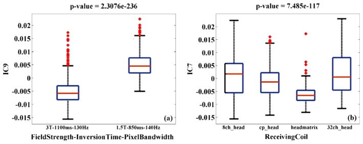
Boxplots of two components exhibiting the most significant scanning effects in the BIG data; (a) IC9 loadings versus magnetic field strength-inversion time-pixel bandwidth; (b) IC7 loadings versus receiving coil.

Table 5.

Talairach regions of the scanning-related components identified in the BIG data (|Z| > 2).

Component	Brain region	Brodmann area	L/R volume (cm3)	L/R random effects, max Z (x,y,z)
IC3 pos	Superior frontal gyrus	8, 6, 9, 10, 11	9.1/10.2	3.73(−6,45,46)/4.07(4,45,46)
	Middle frontal gyrus	9, 6, 8, 10, 46	5.8/5.4	3.12(−30,46,35)/2.77(22,22,58)
	Postcentral gyrus	5, 7, 3, 40, 2, 1	3.4/3.5	2.62(−12,−43,70)/2.60(16,−45,69)
	Inferior parietal lobule	40, 7, 39, 2	2.9/2.8	2.64(−50,−52,50)/2.88(48,−44,54)
	Superior parietal lobule	7	2.3/2.6	2.73(−34,−49,61)/3.01(24,−57,62)
	Precentral gyrus	6, 4, 9, 44	2.1/2.4	2.55(−46,−1,53)/2.57(22,−20,67)
	Precuneus	7, 19, 39, 31	1.3/1.7	2.03(−22,−71,51)/2.51(4,−49,63)
IC3 neg	Lentiform nucleus		3.7/4.8	7.75(−30,−14,1)/8.53(28,−17,3)
	Middle temporal gyrus	21, 20, 39, 37, 22, 19, 38	1.7/1.4	7.29(−42,1,−29)/6.68(53,−37,−3)
	Precuneus	7, 31, 19, 39	1.7/1.1	7.50(−22,−68,33)/5.72(16,−47,34)
	Middle frontal gyrus	10, 46, 8, 6, 11, 9, 47	1.5/0.9	6.36(−32,38,17)/6.35(40,13,20)
	Superior temporal gyrus	22, 13, 38, 39, 21, 41	1.4/0.8	6.18(−53,0,−3)/5.77(46,−42,24)
IC7 pos	Thalamus		4.2/4.4	6.00(−10,−23,1)/6.07(8,−23,1)
	Superior temporal gyrus	22, 41, 13, 39, 38, 21, 42	1.5/1.8	4.75(−50,−17,5)/6.79(44,−25,5)
	Middle temporal gyrus	21, 37, 22, 19, 39, 20	1.9/1.0	3.74(−57,7,−19)/3.65(50,−26,−7)
	Middle frontal gyrus	10, 6, 9, 11, 8, 46, 47	1.1/1.2	4.10(−26,64,6)/3.28(26,32,26)
IC9 pos	Thalamus		2.2/2.7	5.48(−6,−29,−4)/5.54(6,−29,−5)
	Rectal gyrus	11	0.9/1.0	4.80(−10,16,−23)/7.18(4,14,−21)
IC97 pos	Superior temporal gyrus	38, 22, 13, 41, 42, 21, 39	4.2/3.8	6.58(−42,11,−16)/7.18(40,11,−16)
	Anterior cingulate	25, 24, 33, 32	2.7/0.4	6.77(0,6,−5)/4.46(2,3,−10)
	Insula	13, 22, 40, 41, 47	2.4/3.2	5.91(−44,−11,10)/6.40(44,−6,0)
	Parahippocampal gyrus	34, 28, 35, 27, 30, 19, 36, 37	2.3/2.0	8.08(−10,−9,−16)/8.09(10,−7,−18)
	Inferior frontal gyrus	47, 13, 46, 44, 9, 45, 11, 10	1.7/1.8	6.23(−40,15,−16)/6.90(38,13,−17)
	Medial frontal gyrus	25, 10, 9, 6, 11, 8, 32	1.7/0.8	4.66(0,20,−18)/4.72(10,7,−19)
	Thalamus		1.6/0.8	8.26(0,−16,1)/7.77(6,−31,3)
	Cingulate gyrus	24, 32, 31, 23	1.4/0.1	4.80(0,15,27)/3.48(8,−31,35)
	Caudate		1.3/1.2	7.69(−6,10,3)/7.39(6,6,5)

3.2. MCIC data

We applied the same procedure to the MCIC GMC images. 100 ICs were extracted and assessed for associations with the summarized scanning parameters, while controlling for SZ diagnosis. p_th was estimated to be 6.47 × 10⁻³, based on which 8 ICs were identified as scanning-related, as summarized in Table 6. Fig. 4 shows the spatial maps of these ICs, thresholded at |Z| > 2. Again scanning effects were observed at brain edges (IC9, 63 and 92) as well as in the ventricle region, (IC98). For the remaining scanning-related components, Table 7 provides a summary of the Talairach atlas labels of mapped gray matter regions. The most significant scanning effect was observed in IC53 (inferior temporal region), associated with scanner, TR/TE and field strength, among which moderate collinearity was observed (>62% variance explained). Boxplots illustrated that scans acquired with lower field strength and shorter TR exhibited higher regional GMC in IC53, as shown in Fig. 5. Finally these 8 scanning-related components were used for SBM-based data correction.

Table 6.

Scanning effects in the MCIC sMRI data.

Scanning/index of IC	7	9	33	38	53	63	92	98
Scanner	1.31E-02	7.57E-05	6.18E-05	1.22E-02	1.81E-52	2.11E-29	1.41E-08	3.56E-09
Slice thickness	9.01E-03	6.15E-01	5.66E-04	5.30E-02	1.98E-01	7.21E-16	1.25E-06	3.98E-04
TR/TE	2.06E-02	1.94E-05	5.51E-03	5.18E-03	8.62E-53	2.68E-20	2.71E-09	2.96E-04
Number of averages	6.47E-03	1.01E-01	1.87E-03	9.65E-03	5.87E-02	2.90E-19	1.68E-10	4.15E-04
Magnetic field strength	6.40E-02	2.25E-02	1.52E-02	2.54E-03	6.80E-17	1.25E-11	3.54E-06	4.00E-01
RF coil	5.28E-03	1.49E-01	1.37E-03	3.84E-03	5.88E-02	4.14E-21	4.47E-10	4.69E-04
Pixel spacing	6.26E-01	5.07E-01	1.93E-02	8.81E-01	1.84E-06	2.87E-11	3.45E-01	3.49E-02

Note: Significant scanning effects (p ≤ p_th) are highlighted in bold.

Fig. 4.

Spatial maps of the scanning-related components identified in the MCIC data (|Z| > 2).

Table 7.

Talairach regions of the scanning-related components identified in the MCIC data (|Z| > 2).

Component	Brain region	Brodmann area	L/R volume (cm3)	L/R random effects, max Z (x,y,z)
IC7 pos	Middle frontal gyrus	11, 9, 8, 6, 46, 10, 47	2.7/2.1	4.76(−36,40,−10)/4.13(38,21,30)
	Inferior frontal gyrus	47, 9, 44, 45, 13, 10, 46, 11, 6	1.6/1.2	3.83(−55,15,29)/3.91(32,13,−17)
	Superior frontal gyrus	9, 6, 8, 10, 11	1.4/2.1	4.30(−16,58,28)/4.86(16,54,32)
	Superior temporal gyrus	21, 22, 39, 42, 38, 41, 13	1.4/1.9	4.48(−59,−8,−1)/4.34(40,−55,27)
IC7 neg	Middle frontal gyrus	6, 9, 11, 10, 8, 46, 47	2.6/2.4	4.32(−38,27,28)/4.79(28,8,44)
	Middle temporal gyrus	20, 39, 21, 19, 22, 37, 38	2.1/2.2	5.20(−53,−43,−10)/4.97(42,−59,20)
IC33 pos	Middle frontal gyrus	9, 6, 46, 10, 8, 11, 47	5.3/2.8	7.17(−36,13,31)/5.41(36,14,49)
	Superior temporal gyrus	41, 39, 42, 22, 38, 13, 21	3.8/3.0	8.24(−46,−39,6)/5.15(30,8,−29)
	Superior frontal gyrus	8, 6, 10, 11, 9	3.6/2.9	4.55(−12,30,48)/5.52(38,16,47)
	Precuneus	39, 7, 31, 19	3.3/3.0	7.03(−34,−62,36)/4.16(20,−76,28)
	Precentral gyrus	9, 44, 6, 3, 43	3.2/1.6	7.65(−36,11,31)/7.28(48,12,10)
	Middle Temporal gyrus	22, 21, 39, 37, 20, 38, 19	3.0/2.5	7.20(−48,−39,6)/5.96(55,−26,−10)
	Inferior parietal lobule	39, 40, 7, 2	2.6/1.6	7.48(−36,−62,38)/4.45(44,−48,45)
	Inferior frontal gyrus	44, 9, 46, 45, 13, 47, 10, 11, 6	2.2/2.5	6.17(−34,9,29)/7.59(48,12,12)
IC33 neg	Middle frontal gyrus	6, 8, 10, 9, 46, 11, 47	3.3/2.3	5.10(−36,10,47)/4.57(38,14,53)
	Superior frontal gyrus	6, 10, 8, 9, 11	2.8/2.5	4.99(−20,58,25)/5.34(12,22,58)
	Middle temporal gyrus	39, 21, 20, 19, 37, 22, 38	2.2/1.9	5.40(−30,−61,31)/4.75(55,−9,−18)
	Inferior parietal lobule	40, 7, 39	2.2/1.3	6.11(−38,−49,39)/4.23(65,−42,24)
	Precuneus	7, 31, 19, 39	2.0/2.1	8.09(−24,−60,36)/4.63(14,−59,31)
IC38 pos	Middle frontal gyrus	10, 8, 6, 9, 11, 46, 47	3.4/2.6	6.06(−36,39,13)/5.14(32,37,11)
	Superior frontal gyrus	10, 6, 9, 8, 11	2.4/1.9	4.97(−24,44,18)/4.50(20,43,38)
	Cuneus	18, 7, 19, 17, 30, 23	2.2/2.3	6.07(−20,−81,21)/5.55(16,−74,26)
	Parahippocampal gyrus	30, 19, 37, 36, 27, 28, 35, 18	2.1/1.0	5.52(−12,−41,6)/4.35(24,−32,−9)
	Lingual gyrus	19, 18:*, 17, 30	1.9/1.2	4.30(−20,−95,−2)/4.46(16,−47,−3)
	Inferior frontal gyrus	9, 47, 45, 46, 13, 10, 44, 6, 11	1.5/1.8	4.74(−36,9,25)/4.33(30,28,−13)
IC38 neg	Middle frontal gyrus	46, 9, 10, 6, 8, 11, 47	2.9/1.9	4.65(−42,51,14)/3.83(32,23,38)
	Superior frontal gyrus	10, 6, 9, 11, 8	2.1/1.4	5.40(−20,46,23)/4.02(12,56,30)
	Middle temporal gyrus	22, 37, 39, 19, 21, 20, 38	1.8/1.9	4.80(−50,−41,4)/4.12(42,−55,−2)
	Parahippocampal gyrus	30, 35, 27, 36, 28, 34, 19, 37	1.8/0.9	6.64(−8,−39,4)/4.03(10,−41,−1)
	Superior temporal gyrus	38, 39, 21, 41, 22, 42, 13	1.6/1.5	3.56(−46,−39,6)/4.46(24,8,−26)
	Inferior frontal gyrus	45, 44, 47, 10, 9, 11, 13, 46	1.5/1.5	5.66(−38,45,0)/4.65(34,32,−18)
IC53 pos	Inferior temporal gyrus	20, 21, 37, 19	3.5/3.4	10.76(−46,−21,−28)/8.66(46,−21,−28)
	Superior frontal gyrus	11, 6, 10, 8, 9	3.1/2.7	6.24(−8,57,−23)/5.41(10,53,−23)
	Middle frontal gyrus	11, 9, 10, 8, 46, 6, 47	3.0/2.1	4.01(−32,39,11)/4.33(42,48,−14)
	Middle temporal gyrus	38, 39, 22, 21, 20, 37, 19	2.5/2.1	4.46(−36,10,−37)/4.36(55,−47,2)
	Fusiform gyrus	20, 36, 18, 19, 37	2.3/2.6	8.67(−50,−23,−27)/9.08(50,−25,−26)
	Inferior frontal gyrus	47, 9, 11, 45, 46, 13, 44, 10	1.9/1.6	3.72(−50,38,−14)/3.56(53,3,27)
	Superior temporal gyrus	38, 22, 13, 39, 42, 41, 21	1.7/2.4	4.42(−22,10,−36)/5.44(30,4,−39)
IC53 neg	Precentral gyrus	6, 4, 44, 9, 13, 43, 3	3.8/4.2	4.56(−30,−7,52)/4.84(18,−18,65)
	Superior frontal gyrus	6, 8, 11, 9, 10	3.4/2.5	4.64(−8,3,68)/5.54(14,−12,71)
	Middle frontal gyrus	6, 11, 8, 46, 10, 9, 47	2.2/1.2	5.57(−20,−1,61)/4.80(18,−7,59)
	Medial frontal gyrus	6, 9, 10, 8, 25, 32, 11	1.9/2.4	4.64(−6,−20,71)/5.01(6,−20,71)

Fig. 5.

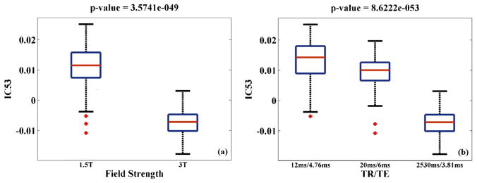
Boxplots of the component exhibiting the most significant scanning effect in the MCIC data; (a) IC53 loadings versus magnetic field strength; (b) IC53 loadings versus TR/TE.

Table 8a summarizes the comparisons among the uncorrected, GLM- and SBM-corrected data in terms of scanning effects evaluated with VBM or ICA. Both GLM and SBM correction appeared to effectively eliminate the scanning effects. Specifically, the VBM analysis did not identify any voxels exhibiting significant scanning effects passing FDR control in either the GLM- or SBM-corrected data. The components extracted by ICA showed greatly reduced proportions of variance explained by the scanning parameters.

Table 8.

Comparisons of the uncorrected, GLM- and SBM-corrected MCIC data in (a) scanning and (b) SZ effects evaluated with ICA or VBM, respectively.

	Uncorrected	GLM-corrected	SBM-corrected
a. Scanning effect (unsmoothed data)
VBM (number of voxels passing FDR)
Scanner	8526	0	0
Slice Thickness	3740	0	0
TR/TE	19491	0	0
Number of Averages	8099	0	0
Magnetic Field Strength	19487	0	0
Receiving Coil	3739	0	0
Pixel Spacing	363	0	0
ICA (Proportion of variance explained)
Scanner	61.99%	0.90%	3.45%
Slice Thickness	27.43%	3.06%	2.86%
TR/TE	61.39%	0.86%	1.88%
Number of Averages	29.47%	0.64%	3.33%
Magnetic Field Strength	57.87%	0.42%	1.68%
Receiving Coil	8.28%	0.14%	2.36%
Pixel Spacing	19.02%	3.05%	3.28%
b. SZ effect (smoothed data)
VBM (number of voxels passing FDR)	64,632	64,632	31,858
ICA (Proportion of explained variance)	11.63% (IC18)	12.34% (IC20)	16.18% (IC2)
	8.84% (IC5*)	10.11% (IC5*)
	5.63% (IC7*)	7.74% (IC7*)

Note: The most significant SZ components, IC18-Uncorrected_S, IC20-GLM_S and IC2-SBM_S (highlighted in bold) are summarized in Fig. 7. Fig. 8 shows the spatial maps of IC5-Uncorrected_S, IC7-Uncorrected_S as well as IC5-GLM_S and IC7-GLM_S exhibiting questionable SZ effects.

Table 8b presents the performance comparisons in terms of SZ effects among the uncorrected, GLM- and SBM-corrected data, all of which had been firstly smoothed. In the VBM analysis, the uncorrected and GLM-corrected data yielded the same 64,632 voxels exhibiting significant SZ effects after FDR control, while the SBM-corrected data yielded 31,858 voxels. Fig. 6 illustrates the spatial maps of voxels identified as SZ-related in the uncorrected or GLM-corrected data, but not in the SBM-corrected data. When evaluated by ICA, the SBM-corrected data presented more significant SZ effect, where the most discriminating component IC2-SBM_S (the subscript _S stands for ‘smoothed’) explained an increased proportion of variance in SZ diagnosis (16.18%) compared to those obtained from the uncorrected (11.63% for IC18-Uncorrected_S) and GLM-corrected data (12.34% for IC20-GLM_S), as highlighted in Table 8b. Fig. 7 shows the spatial maps of these SZ-discriminating components (thresholded at |Z| > 2). Boxplots are also provided to demonstrate the group differences between patients and controls. Among these SZ-discriminating components, the mapped brain regions were consistent, highlighting a frontal-temporal network. Besides, the uncorrected and GLM-corrected data also presented marginal SZ effects captured by IC5 and 7, whose spatial maps are illustrated in Fig. 8.

Fig. 6.

A spatial map of the SZ-related voxels identified with VBM (FDR control) in the uncorrected or GLM-corrected, but not in the SBM-corrected data.

Fig. 7.

Spatial maps (|Z| > 2) and boxplots of the most significant SZ-discriminating components identified in the uncorrected (IC18), GLM-corrected (IC20) and SBM-corrected (IC2) data after smoothing. All the components are spatially consistent, highlighting the frontal temporal network.

Fig. 8.

Spatial maps of questionable SZ-discriminating components identified in the uncorrected and GLM-corrected data after smoothing.

4. Discussion

In this study, we explored the effects of various scanning parameters in multi-site GMC data and determined if a correction is applicable in the SBM framework. The exploration was performed with GMC images collected from 1460 healthy subjects from the BIG study. As expected, we observed significant scanning effects in distributed brain regions. The most pronounced effect was observed from magnetic field strength. More interestingly, receiving coil presented an independent effect which was not captured by scanner or field strength. In the second study with the MCIC data of 110 SZ patients and 124 healthy controls, the results to some extent echoed the BIG findings, highlighting scanning effects around ventricle, brainstem and inferior temporal regions, and at brain edges. Meanwhile, some differences were also noted. For instance, in the MCIC data, no significant scanning effect was identified in thalamus as for the BIG data. This might be due to different scanning platforms such that the effect was not significant in the resulting images. In addition, it was also demonstrated with the MCIC data that the SBM approach effectively separated scanning effects from the SZ-related GMC changes, thus enabling a correction which helped improve the significance of SZ effect.

4.1. BIG data

The most significant scanning effect was observed in IC9. This component highlighted the brainstem region, where the GMC exhibited differences among subjects scanned at various stations, which primarily involved discrepancies in magnetic field strength, inversion time and pixel bandwidth. Magnetic field strength affects the T₁-relaxation and, hence, the imaging contrast between gray and white matter (Duewell et al., 1996), which is consistent with our observation. Higher field strength also results in increased magnetic susceptibility artifacts (Bernstein et al., 2006). The brainstem is particularly prone to these artifacts (Focke et al., 2011), which can cause geometric distortions, signal loss as well as influence the effective excitation field and flip angle, thus affecting contrast in T₁-weighted images (Truong et al., 2006). Inversion time is typically chosen in line with T₁-relaxation (and hence field strength) as it determines the magnetization before excitation in each tissue, and thus the T₁-contrast. Pixel bandwidth, or receiver bandwidth, refers to the difference in magnetic resonance frequencies between adjacent pixels. This parameter is most commonly associated with chemical shift between fat and water and has a direct effect on image SNR (Schmitz et al., 2005). In the present study, it is difficult to disentangle the effects of individual parameters due to collinearity. However, it appears likely that the GMC variability observed in brainstem region is majorly attributable to the inversion time-field strength interaction.

A second notable scanning effect was observed in IC7. This component highlighted the thalamus region and reflected GMC variability induced by RF coils, especially the receiving coil. As illustrated in Table 1, 1259 out of the 1460 BIG participants were scanned using the same type of transmitting coil. Therefore, the present data may not appropriately reflect how transmitting coil influences the image pattern. Moreover, effects of transmitting coil only become more substantial at 7 T or higher (Vaughan et al., 2001). Regarding the receiving coil, Fig. 3b shows that subjects scanned with 32-channel head coil exhibited higher GMC in the highlighted thalamus region of IC7. Meanwhile it is noteworthy that IC7 was the only component associated with SNR (r = 0.26, p = 1.40 × 10⁻²³). Not surprisingly, SNR exhibited a significant group difference among different types of receiving coils (p = 3.28 × 10⁻⁴⁶), where the 32-channel head coil yielded the highest overall SNR and the 8-channel head coil the second. This observation is consistent with previous studies that have found spatially dependent gains in SNR with the addition of element coils in multichannel phased-array head coils (de Zwart et al., 2004; Wintersperger et al., 2006). Overall, our finding reveals interrelationships between SNR and RF-receiving coil, and indicates that coil design may lead to a significant variability in the image pattern. Most importantly, it is clearly demonstrated that discrepancies in individual scanning parameters can present unique effects not captured by a single variable of ‘site’ or ‘scanner’. Therefore, it is strongly recommended that in addition to calibrating magnetic field strength and inversion time, inconsistency in RF coil designs should be avoided in aggregated structural MRI analyses whenever possible. Otherwise, individual scanning parameters should be assessed to avoid false positive findings.

4.2. MCIC data

The MCIC study confirmed significant systematic differences in the image pattern induced by individual scanning parameters. The most affected component was IC53, highlighting the inferior temporal region and showing a relationship with scanner and field strength. Note that scanner was completely collinear with pixel bandwidth, and scanning sequence completely collinear with TR/TE and flip angle in the MCIC data. Magnetic field strength, as discussed above, can significantly influence the T₁-contrast. The observation in the MCIC data is consistent with the BIG data in that scans obtained with lower field strength exhibited higher regional GMC, as shown in Fig. 5a. Repetition time determines the recovery of magnetization and directly affects the T₁-contrast. The box-plot with TR/TE (Fig. 5b) illustrates that MCIC scans acquired with shorter repetition time exhibited higher regional GMC, consistent with the general concept of shorter TR leading to higher contrast. In contrast, no linear relation was observed between the component loadings and TE, suggesting that the image variability was more likely attributable to repetition time rather than echo time. Although due to collinearity we could not determine which parameter is the major contributor to the image variability observed in IC53, the results confirmed that inconsistency in field strength and sequence design can introduce significant systematic differences in multi-site sMRI studies (Fennema-Notestine et al., 2007; Stonnington et al., 2008) and should be best avoided.

After SBM-correction, no significant scanning effects were observed and the SZ effect was refined when evaluated with ICA, where the identified component explained a larger proportion of variance in SZ diagnosis, as shown in Table 8a and 8b. The most SZ-discriminating component identified in the SBM-corrected data, IC2-SBM_S, was spatially consistent with IC18-Uncorrected_S and IC20-GLM_S, as shown in Fig. 7. All these three components suggested SZ-related gray matter reduction in a frontal-temporal network, one of the most consistently identified structural variations for the disease (Cannon et al., 2002; Glahn et al., 2008; Kuperberg et al., 2003; Turner et al., 2012; Xu et al., 2009). The GLM- and SBM-corrected data presented more significant group differences in the frontal-temporal network compared to the uncorrected data, suggesting that correcting for confounding effects might help refine the true effect of interest. Meanwhile, the uncorrected and GLM-corrected data also presented other SZ effects, as illustrated in Table 8b and Fig. 8. IC5-GLM_S resembled IC5-Uncorrected_S, both highlighting voxels at edges of the frontal region. IC7-Uncorrected_S reflected sparsely scattered small clusters of voxels, and IC7-GLM_S highlighted brainstem where scanning effects were observed. Overall, the validity of these SZ-related components is highly questionable. In contrast, the SBM-corrected data presented one reliable frontal-temporal network exhibiting the most significant SZ effect, suggesting that the data were more effectively corrected.

The evaluation with VBM echoed the results obtained with the ICA approach. Both GLM- and SBM-correction effectively reduced the scanning effects. On the other hand, the uncorrected and GLM-corrected data presented more SZ-related voxels than the SBM-corrected data, as illustrated in Table 8b. Fig. 6 provides a slice view of the voxels not identified in the SBM-corrected data. Clearly the SBM-missing voxels were majorly localized to brain edges, brainstem, cerebellum and paranasal sinus. And, these missing voxels corresponded to those highlighted in some of the identified scanning-related components, including IC7-Uncorrected and IC53-Uncorrected, which also showed marginal SZ effects (p = 3.08 × 10⁻⁴ and 4.51 × 10⁻⁴, respectively). As these components were eliminated in the SBM correction, no significant effects would be expected in those regions in the subsequent VBM analysis of SZ effect.

The comparison between GLM and SBM correction demonstrates that the former is more model-based while the latter is more data-driven. In a GLM model, all the variance that can be explained by the predictors is regressed out. As shown in Table 8a, the variances explained by the scanning parameters are less in the GLM-corrected data than in the SBM-corrected data, although both are not significant. However, one concern is that the GLM model is not able to deal with embedded collinearity, such that variances shared between scanning parameters and traits of interest may also be eliminated. In contrast, in the SBM model, ICA extracts components attributed to different sources where the covariations among voxels, therefore the systematic changes over the brain are emphasized. Thus, the overlap between scan effects and (possibly multiple) effects of interest is allowed. For instance, the GLM approach could not separate the SZ-related voxels from each other, while ICA acknowledged that they covaried with different underlying patterns such that the SZ effect was split into IC7 (p = 3.08 × 10⁻⁴), IC53 (p = 4.51 × 10⁻⁴), IC94 (p = 1.94 × 10⁻⁶) and IC98 (p = 5.96 × 10⁻⁶) in the unsmoothed uncorrected data (see Fig. 4 for IC7, 53 and 98; see Fig. S2 for IC94). Subsequent analyses suggested that IC94-Uncorrected showed no significant scanning effects, while others were likely confounded, as illustrated in Table 6. Overall, the data-driven nature is likely why SBM showed a better performance in improving the effect of interest in this SZ study. It enables researchers to recognize the heterogeneity and allows flexibility in whether a correction is necessary for an individual component.

Limitations of the study lie in the following aspects. First, the image variability in multi-site studies is the final manifestation of a complex interplay between multiple factors. We show that ICA can be a very helpful tool in this regard. However, as a linearly additive model, ICA only deals with linear scanning effects, which has been a common practice in the field (Fennema-Notestine et al., 2007; Pardoe et al., 2008; Stonnington et al., 2008; Takao et al., 2013). More efforts are awaited to address nonlinear effects. Second, some scanning-related variance might still be retained after the correction. One possibility is that some effects might be ignored if the contributing scanning parameter is not taken into account, which emphasizes the importance of completely examining the scanning settings and generating a reliable design matrix for the purpose of detecting scanning effects. Also it is possible that some marginal scanning effects may not be eliminated if they miss the selected threshold p-value, though these marginal effects are not expected to be a major source of bias and can be mitigated by co-variation in post hoc analyses. Finally, the results of this study were developed on gray matter concentration data. However, we also evaluated the images from a modulated preprocessing step, and found the identified scanning effects were highly consistent (not shown). 8 scanning-related components were identified in the modulated images, 7 of which showed similar spatial patterns to those observed in the unmodulated data. Again the component highlighting brainstem showed the most significant effect. These observations suggested that the identified image variability is not highly sensitive to the preprocessing and more likely induced by the scanning process.

In summary, our study explored scanning effects in multi-site structural MRI studies and demonstrated an effective approach for correction. The results confirm that inconsistent magnetic field strength, sequence design and RF-receiving coil can all induce significant image variability and deserve more attention in the current atmosphere of data sharing and aggregation for large-scale analyses. For aggregated studies where discrepancies exist in scanning platforms, our work justifies the importance of including individual scanning parameters, instead of a single ‘site’ or ‘scanner’ variable, as covariates for the evaluation of confounding effects. Finally, SBM proves a flexible and effective data-driven approach to detect and correct scanning effects, which holds the promise to reduce the risk of false positives and enhance the true effect of interest.

HIGHLIGHTS.

• Explored how scanning settings affect the image pattern in multi-site sMRI studies.

• A data-driven SBM correction was designed and tested.

• Consistent field strength, sequence design and RF coil are strongly recommended.

• SBM proves a flexible and effective approach to detect and clean scanning effects.

Appendix A. Supplementary data

Supplementary data associated with this article can be found, in the online version, at http://dx.doi.org/10.1016/j.jneumeth.2014.04.023.

References

- Amari S. Natural gradient works efficiently in learning. Neural Comput. 1998;10:251–76. [Google Scholar]
- Andreasen NC, Flaum M, Arndt S. The comprehensive assessment of symptoms and history (Cash) – an instrument for assessing diagnosis and psychopathology. Arch Gen Psychiatry. 1992;49:615–23. doi: 10.1001/archpsyc.1992.01820080023004. [DOI] [PubMed] [Google Scholar]
- Ashburner J, Friston KJ. Voxel-based morphometry—the methods. Neuroimage. 2000;11:805–21. doi: 10.1006/nimg.2000.0582. [DOI] [PubMed] [Google Scholar]
- Ashburner J, Friston KJ. Unified segmentation. Neuroimage. 2005;26:839–51. doi: 10.1016/j.neuroimage.2005.02.018. [DOI] [PubMed] [Google Scholar]
- Bell AJ, Sejnowski TJ. An information-maximization approach to blind separation and blind deconvolution. Neural Comput. 1995;7:1129–59. doi: 10.1162/neco.1995.7.6.1129. [DOI] [PubMed] [Google Scholar]
- Bernstein MA, Huston J, 3rd, Ward HA. Imaging artifacts at 3.0 T. J Magn Reson Imaging. 2006;24:735–46. doi: 10.1002/jmri.20698. [DOI] [PubMed] [Google Scholar]
- Button KS, Ioannidis JPA, Mokrysz C, Nosek BA, Flint J, Robinson ESJ, et al. Power failure: why small sample size undermines the reliability of neuroscience. Nat Rev Neurosci. 2013;14:365–76. 444. doi: 10.1038/nrn3475. [DOI] [PubMed] [Google Scholar]
- Cannon TD, Thompson PM, van Erp TGM, Toga AW, Poutanen VP, Huttunen M, et al. Cortex mapping reveals regionally specific patterns of genetic and disease-specific gray-matter deficits in twins discordant for schizophrenia. Proc Natl Acad Sci USA. 2002;99:3228–33. doi: 10.1073/pnas.052023499. [DOI] [PMC free article] [PubMed] [Google Scholar]
- de Zwart JA, Ledden PJ, van Gelderen P, Bodurka J, Chu R, Duyn JH. Signal-to-noise ratio and parallel imaging performance of a 16-channel receive-only brain coil array at 3.0 T. Magn Reson Med: Off J Soc Magn Reson Med/Soc Magn Reson Med. 2004;51:22–6. doi: 10.1002/mrm.10678. [DOI] [PubMed] [Google Scholar]
- Duewell S, Wolff SD, Wen H, Balaban RS, Jezzard P. MR imaging contrast in human brain tissue: assessment and optimization at 4 T. Radiology. 1996;199:780–6. doi: 10.1148/radiology.199.3.8638005. [DOI] [PubMed] [Google Scholar]
- Fennema-Notestine C, Gamst AC, Quinn BT, Pacheco J, Jernigan TL, Thal L, et al. Feasibility of multi-site clinical structural neuroimaging studies of aging using legacy data. Neuroinformatics. 2007;5:235–45. doi: 10.1007/s12021-007-9003-9. [DOI] [PubMed] [Google Scholar]
- Ferreira LK, Diniz BS, Forlenza OV, Busatto GF, Zanetti MV. Neurostructural predictors of Alzheimer’s disease: a meta-analysis of VBM studies. Neurobiol Aging. 2011;32:1733–41. doi: 10.1016/j.neurobiolaging.2009.11.008. [DOI] [PubMed] [Google Scholar]
- First MB, Gibbon M, Spitzer RL, Williams JBW, Benjamin LS. Structured clinical interview for DSM-IV axis II personality disorders, (SCID-II) 4. Washington, DC: American Psychiatric Press; 1997. [Google Scholar]
- Focke NK, Helms G, Kaspar S, Diederich C, Toth V, Dechent P, et al. Multi-site voxel-based morphometry—not quite there yet. Neuroimage. 2011;56:1164–70. doi: 10.1016/j.neuroimage.2011.02.029. [DOI] [PubMed] [Google Scholar]
- Fornito A, Yucel M, Dean B, Wood SJ, Pantelis C. Anatomical abnormalities of the anterior cingulate cortex in schizophrenia: bridging the gap between neuroimaging and neuropathology. Schizophr Bull. 2009;35:973–93. doi: 10.1093/schbul/sbn025. [DOI] [PMC free article] [PubMed] [Google Scholar]
- Giuliani NR, Calhoun VD, Pearlson GD, Francis A, Buchanan RW. Voxel-based morphometry versus region of interest: a comparison of two methods for analyzing gray matter differences in schizophrenia. Schizophr Res. 2005;74:135–47. doi: 10.1016/j.schres.2004.08.019. [DOI] [PubMed] [Google Scholar]
- Glahn DC, Laird AR, Ellison-Wright I, Thelen SM, Robinson JL, Lancaster JL, et al. Meta-analysis of gray matter anomalies in schizophrenia: application of anatomic likelihood estimation and network analysis. Biol Psychiatry. 2008;64:774–81. doi: 10.1016/j.biopsych.2008.03.031. [DOI] [PMC free article] [PubMed] [Google Scholar]
- Gollub RL, Shoemaker JM, King MD, White T, Ehrlich S, Sponheim SR, et al. The MCIC collection: a shared repository of multi-modal, multi-site brain image data from a clinical investigation of schizophrenia. Neuroinformatics. 2013;11:367–88. doi: 10.1007/s12021-013-9184-3. [DOI] [PMC free article] [PubMed] [Google Scholar]
- Good CD, Johnsrude IS, Ashburner J, Henson RNA, Friston KJ, Frackowiak RSJ. A voxel-based morphometric study of ageing in 465 normal adult human brains. Neuroimage. 2001;14:21–36. doi: 10.1006/nimg.2001.0786. [DOI] [PubMed] [Google Scholar]
- Henkelman RM. Measurement of signal intensities in the presence of noise in MR images. Med Phys. 1985;12:232–3. doi: 10.1118/1.595711. [DOI] [PubMed] [Google Scholar]
- Honea R, Crow TJ, Passingham D, Mackay CE. Regional deficits in brain volume in schizophrenia: a meta-analysis of voxel-based morphometry studies. Am J Psychiatry. 2005;162:2233–45. doi: 10.1176/appi.ajp.162.12.2233. [DOI] [PubMed] [Google Scholar]
- Jovicich J, Czanner S, Greve D, Haley E, van der Kouwe A, Gollub R, et al. Reliability in multi-site structural MRI studies: effects of gradient non-linearity correction on phantom and human data. Neuroimage. 2006;30:436–43. doi: 10.1016/j.neuroimage.2005.09.046. [DOI] [PubMed] [Google Scholar]
- Kalpouzos G, Chetelat G, Baron JC, Landeau B, Mevel K, Godeau C, et al. Voxel-based mapping of brain gray matter volume and glucose metabolism profiles in normal aging. Neurobiol Aging. 2009;30:112–24. doi: 10.1016/j.neurobiolaging.2007.05.019. [DOI] [PubMed] [Google Scholar]
- Kuperberg GR, Broome MR, McGuire PK, David AS, Eddy M, Ozawa F, et al. Regionally localized thinning of the cerebral cortex in schizophrenia. Arch Gen Psychiatry. 2003;60:878–88. doi: 10.1001/archpsyc.60.9.878. [DOI] [PubMed] [Google Scholar]
- Lancaster JL, Rainey LH, Summerlin JL, Freitas CS, Fox PT, Evans AC, et al. Automated labeling of the human brain: a preliminary report on the development and evaluation of a forward-transform method. Hum Brain Mapp. 1997;5:238–42. doi: 10.1002/(SICI)1097-0193(1997)5:4<238::AID-HBM6>3.0.CO;2-4. [DOI] [PMC free article] [PubMed] [Google Scholar]
- Lancaster JL, Woldorff MG, Parsons LM, Liotti M, Freitas CS, Rainey L, et al. Automated Talairach atlas labels for functional brain mapping. Hum Brain Mapp. 2000;10:120–31. doi: 10.1002/1097-0193(200007)10:3<120::AID-HBM30>3.0.CO;2-8. [DOI] [PMC free article] [PubMed] [Google Scholar]
- Littmann A, Guehring J, Buechel C, Stiehl HS. Acquisition-related morphological variability in structural MRI. Acad Radiol. 2006;13:1055–61. doi: 10.1016/j.acra.2006.05.001. [DOI] [PubMed] [Google Scholar]
- Luders E, Narr KL, Thompson PM, Woods RP, Rex DE, Jancke L, et al. Mapping cortical gray matter in the young adult brain: effects of gender. Neuroimage. 2005;26:493–501. doi: 10.1016/j.neuroimage.2005.02.010. [DOI] [PubMed] [Google Scholar]
- Maguire EA, Gadian DG, Johnsrude IS, Good CD, Ashburner J, Frackowiak RS, et al. Navigation-related structural change in the hippocampi of taxi drivers. Proc Natl Acad Sci USA. 2000;97:4398–403. doi: 10.1073/pnas.070039597. [DOI] [PMC free article] [PubMed] [Google Scholar]
- Moorhead TW, Gountouna VE, Job DE, McIntosh AM, Romaniuk L, Lymer GK, et al. Prospective multi-centre voxel based morphometry study employing scanner specific segmentations: procedure development using CaliBrain structural MRI data. BMC Med Imaging. 2009;9:8. doi: 10.1186/1471-2342-9-8. [DOI] [PMC free article] [PubMed] [Google Scholar]
- Pardoe H, Pell GS, Abbott DF, Berg AT, Jackson GD. Multi-site voxel-based morphometry: methods and a feasibility demonstration with childhood absence epilepsy. Neuroimage. 2008;42:611–6. doi: 10.1016/j.neuroimage.2008.05.007. [DOI] [PMC free article] [PubMed] [Google Scholar]
- Schmitz BL, Aschoff AJ, Hoffmann MH, Gron G. Advantages and pitfalls in 3 T MR brain imaging: a pictorial review. Am J Neuroradiol. 2005;26:2229–37. [PMC free article] [PubMed] [Google Scholar]
- Segall JM, Turner JA, van Erp TG, White T, Bockholt HJ, Gollub RL, et al. Voxel-based morphometric multisite collaborative study on schizophrenia. Schizophr Bull. 2009;35:82–95. doi: 10.1093/schbul/sbn150. [DOI] [PMC free article] [PubMed] [Google Scholar]
- Sowell ER, Peterson BS, Thompson PM, Welcome SE, Henkenius AL, Toga AW. Mapping cortical change across the human life span. Nat Neurosci. 2003;6:309–15. doi: 10.1038/nn1008. [DOI] [PubMed] [Google Scholar]
- Stonnington CM, Tan G, Kloppel S, Chu C, Draganski B, Jack CR, Jr, et al. Interpreting scan data acquired from multiple scanners: a study with Alzheimer’s disease. Neuroimage. 2008;39:1180–5. doi: 10.1016/j.neuroimage.2007.09.066. [DOI] [PMC free article] [PubMed] [Google Scholar]
- Takao H, Hayashi N, Ohtomo K. Effects of study design in multi-scanner voxel-based morphometry studies. Neuroimage. 2013;84C:133–40. doi: 10.1016/j.neuroimage.2013.08.046. [DOI] [PubMed] [Google Scholar]
- Truong TK, Chakeres DW, Beversdorf DQ, Scharre DW, Schmalbrock P. Effects of static and radiofrequency magnetic field inhomogeneity in ultra-high field magnetic resonance imaging. Magn Reson Imaging. 2006;24:103–12. doi: 10.1016/j.mri.2005.09.013. [DOI] [PubMed] [Google Scholar]
- Turner JA, Calhoun VD, Michael A, van Erp TG, Ehrlich S, Segall JM, et al. Heritability of multivariate gray matter measures in schizophrenia. Twin Res Hum Genet: Off J Int Soc Twin Stud. 2012;15:324–35. doi: 10.1017/thg.2012.1. [DOI] [PMC free article] [PubMed] [Google Scholar]
- Vaughan JT, Garwood M, Collins CM, Liu W, DelaBarre L, Adriany G, et al. 7 T versus 4 T: RF power, homogeneity, and signal-to-noise comparison in head images. Magn Reson Med: Off J Soc Magn Reson Med/Soc Magn Reson Med. 2001;46:24–30. doi: 10.1002/mrm.1156. [DOI] [PubMed] [Google Scholar]
- Vovk U, Pernus F, Likar B. A review of methods for correction of intensity inhomogeneity in MRI. IEEE Trans Med Imaging. 2007;26:405–21. doi: 10.1109/TMI.2006.891486. [DOI] [PubMed] [Google Scholar]
- Wintersperger BJ, Reeder SB, Nikolaou K, Dietrich O, Huber A, Greiser A, et al. Cardiac CINE MR imaging with a 32-channel cardiac coil and parallel imaging: impact of acceleration factors on image quality and volumetric accuracy. J Magn Reson Imaging. 2006;23:222–7. doi: 10.1002/jmri.20484. [DOI] [PubMed] [Google Scholar]
- Xu L, Groth KM, Pearlson G, Schretlen DJ, Calhoun VD. Source-based morphometry: the use of independent component analysis to identify gray matter differences with application to Schizophrenia. Hum Brain Mapp. 2009;30:711–24. doi: 10.1002/hbm.20540. [DOI] [PMC free article] [PubMed] [Google Scholar]
Associated Data
This section collects any data citations, data availability statements, or supplementary materials included in this article.