Network Firewall Dynamics and the Subsaturation Stabilization of HIV

Abstract

In 2001, Friedman et al. conjectured the existence of a “firewall effect” in which individuals who are infected with HIV, but remain in a state of low infectiousness, serve to prevent the virus from spreading. To evaluate this historical conjecture, we develop a new graph-theoretic measure that quantifies the extent to which Friedman's firewall hypothesis(FH)holds in a risk network. We compute this new measure across simulated trajectories of a stochastic discrete dynamical system that models a social network of 25,000 individuals engaging in risk acts over a period of 15 years. The model's parameters are based on analyses of data collected in prior studies of the real-world risk networks of people who inject drugs (PWID) in New York City. Analysis of system trajectories reveals the structural mechanisms by which individuals with mature HIV infections tend to partition the network into homogeneous clusters (with respect to infection status) and how uninfected clusters remain relatively stable (with respect to infection status) over long stretches of time. We confirm the spontaneous emergence of network firewalls in the system and reveal their structural role in the nonspreading of HIV.

1. Introduction

Social network research among people who inject drugs (PWID) has produced considerable data on HIV-1 infection profiles and equally detailed data on the broad demographic and behavioral profiles of injecting communities and their risk behaviors. However, prior research has not—and for reasons of cost often cannot—produce long-term, dynamic data on these same populations. Risk networks—graphs whose vertices are individuals and edges are social connections bearing disease transmission risk—are now widely recognized as a critical construct in understanding infection patterns [1, 2], as they represent the natural environment in which risk behaviors take place and through which infection propagates. Such a representation shifts our view of risk away from individual behaviors to collective, social bodies as the carriers and transmitters of infections [3, 4]. Modeling risk networks as (stochastic) discrete dynamical systems provides an opportunity to understand (through both analysis and simulation) the long-term behavior of PWID risk networks themselves—well beyond what can be seen by considering their constituent individuals in isolation.

HIV has been investigated extensively in a number of PWID communities, including New York City [5], where there was a rapid initial spread of the virus among PWID in the early 1980s, but where HIV prevalence stabilized to between 40 and 50% (i.e., at much lower than 100% or “saturation” levels), despite the fact that risk behaviors could result in infection remained common [6]. One interesting aspect of HIV's natural history is the fact that its viral burden has a tendency to transition from an acute, highly infectious phase to a chronic phase where overall infectiousness is much lower. Real-world PWID risk networks exhibit interesting characteristics as well, including a high degree of clustering [7]. The challenge taken up by us in the present work is to make evident how subsaturation stabilization comes about within the proposed stochastic discrete dynamical system, through the complex interplay of the natural history of HIV and PWID risk network dynamics.

Outline. In Section 2, we develop a stochastic discrete dynamical system that models HIV propagation in a PWID risk network, setting its parameters based on data gathered in an earlier study on Social Factors for HIV Risk in New York City [6]. In Section 3, we design a (macrolevel) graph-theoretic formalization of Friedman et al.'s firewall hypothesis (FH). In Section 4, we determine the extent to which FH is manifested in the stochastic discrete dynamical system, by sampling its trajectories via simulation. Finding the hypothesis tenable, in Section 5 we proceed to dissect the system trajectories to reveal the structural mechanisms behind the emergence of the FH phenomenon and its role in the continued regulation of HIV propagation within PWID risk networks.

2. Mathematical Model

The mathematical model underlying the stochastic discrete dynamical system consists of three parts: (i) the network model describes what real-world PWID risk networks “look like” and how to create artificial ones which may serve as plausible and interesting initial states of the system; this is the subject of Section 2.1; (ii) the dynamism model describes the evolution of system trajectories by specifying how PWID risk networks restructure themselves over time in response to the departure and arrival of individuals; this is the subject of Section 2.2; (iii) the infection model describes the evolution of system trajectories by formalizing the process by which HIV spreads as a consequence of individual risk acts; this is the subject of Section 2.3.

2.1. Network Model

Within a PWID risk network, each node is an individual and each edge represents a relationship that bears the potential for injection drug couse—referred to hereafter as risk relationship. The network model specifies the process by which we construct plausible PWID risk networks that may serve as initial states (i.e., from which trajectories of the stochastic discrete dynamical system may be fruitfully generated). The network model consists of four parts: (A) obtain data on real-world PWID risk networks, (B) define a statistical network model, (C) specify model parameters based on real-world PWID risk network data, and finally, (D) generate new artificial PWID risk networks using the parametrized model. In what follows, we describe each of these four parts in greater detail.

In what follows, we adhere to the standard mathematical conventions: given a set d835dc46, we denote its cardinality by |S|. Given two sets d835S, T, we denote by S × T the set of all ordered pairs (s, t), where s ∈ S and t ∈ T. A function f with domain D and range R is so declared by the assertion f : D → R. Given a subset Y ⊆ R, the set f⁻¹(Y) is defined to be the set of elements x ∈ D for which f(x) ∈ Y.

(A) Obtaining Data on Real-World Risk Networks. We view a risk network as a combinatorial fabric, weaving together a set of ,n individuals, each of whom has m properties, and where each individual may host an instance of the pathogen. A human population V may be surveyed in order to map out its instantaneous state: each constituent individual ν being interrogated about a fixed set of m attributes X = {x₁, . . . , x_m}; for example, x₁ could be gender, while x₂ might be age, and so on We assume that each variable x_i (for i = 1, . . . , m)is categorical, taking values from a finite set U_i that is known in advance (e.g., U₁ could be {Male,Female}, while U₂ might be {21AndUnder, Over21}). Each node attribute x_d835dc56 (i = 1, . . . , m) is viewed as a function x_i : V → U_i. To model a risk network, the survey process must go beyond individual attributes and collect data on the risk relationships between individuals. In practice, during the survey, each individual ν from V is asked to provide sufficient information required to identify the individuals N(ν) ⊆ V with whom ν has a risk relationship. In other words, the survey must capture individual ego network data that can then be aggregated to define the risk network as a whole. By collecting data on N(ν) in the survey, we are able to specify d : V → N, where d(ν) = |N(ν)| is the number of risk relationships ν has. The set of all risk relationships is then expressible as E = ⋃_ν∈V N(ν). Finally, the survey must collect data on disease prevalence by identifying the set of individuals A ⊆ V who are afflicted by the particular pathogen of interest. Collecting the above elements, we define a risk network to be the (m + 4) tuple $\mathcal{D}$ = (x_i, V, E, A, d), where i = 1, . . . , m.

In the context of this work, we drew upon data collected in the Social Factors and HIV Risk study (SFHR). Conducted between 1990 and 1993, SFHR was a cross-sectional, mixed methods project that asked 767 out-of-treatment intravenous drug users about their risk networks and HIV risk behaviors in the prior 30 days. Interested in both individuals’ network composition (namely, the presence of high-risk partners) and sociometric risk position, the SFHR study produced several major findings relevant to risk populations with high HIV prevalence and low secondary incidence [8–15]. SFHR documented 662 connections between study participants (which after symmetrizing and eliminating duplicates yielded a set of 1032 edges). These edges partitioned the study subjects into 92 connected components, including a large connected component of 230 individuals containing a 105-member 2-core exhibiting higher HIV prevalence [2].

(B) Defining a Statistical Network Model. In modeling a risk network $\mathcal{D}$, the question arises as to the “appropriate” contents of the model, particularly, which m attributes X = {x₁, . . . , x_m} are significantly influential in the formation of risk relationships? To this end, the statistical analysis of network data has been advanced considerably by the introduction of Exponential Random Graph Modeling (ERGM), a statistical technique aimed at determining the extent to which the likelihood of network linkages appears to be biased towards (or against) the creation of specified network substructures (above and beyond what is expected by chance). Such substructures can be as simple as the tendency of “like” nodes to be connected (at a greater rate than expected by a random distribution of connections), or as complex as specific structures of connection between sets of individuals [16]. The theoretical basis for ERGM analysis has been known for some time [17, 18], with estimation questions settled recently [19]; several detailed expositions of ERGM are available [20–22].

Given a risk network $\mathcal{D}$ = (x_i, V, E, A, d), where (i = 1, . . . , m), we can from each of the attributes x_i determining a univariate attribute distribution α_i : U_i → [0, 1], defined such that for u ∈ U_i

$${\alpha }_i\left(u\right)\stackrel{\mathrm{def}}{=}\frac{\mid x_i^{-1}\left(u\right)\mid }{\mid V\mid }.$$ (1)

The relationships E define m bivariate attribute distributions β_i : U_i × U_i → [0, 1], wherein for each for u₁, u₂ ∈ U_i

$${\beta }_i(u_1,u_2)\stackrel{\mathrm{def}}{=}\frac{\mid (x_i^{-1}\left(u_1\right)\times x_i^{-1}\left(u_2\right))\cap E\mid }{\mid E\mid }.$$ (2)

The set E also implicitly defines a univariate degree distribution $\chi :\mathbb{Z}\times \mathbb{Z}\to \mathbb{R}$ where for integers a < b we take

$$\chi (a,b)\stackrel{\mathrm{def}}{=}\frac{\mid \{v\in V\mid a\le d\left(v\right)<b\}\mid }{\mid V\mid },$$ (3)

and a bivariate degree distribution $\overline{\overline{\chi }}:{(\mathbb{Z}\times \mathbb{Z})}^2\to \mathbb{R}$ where for every 4-tuple of integers a < b, a^′ < b^′ we take

$$\overline{\overline{\chi }}(a,b,a^{\prime },b^{\prime })\stackrel{\mathrm{def}}{=}\frac{\mid \{e\in E\mid e=(u,v);a\le d\left(u\right)<b;a^{\prime }\le d\left(v\right)<b^{\prime }\}\mid }{\mid E\mid }.$$ (4)

Finally, we compute pathogen prevalence p ∈ [0, 1] as

$$p\stackrel{\mathrm{def}}{=}\frac{\mid A\mid }{\mid V\mid }.$$ (5)

The statistical network model $\mathcal{M}\left(\mathcal{D}\right)$ derived from risk network $\mathcal{D}$ is taken to be the (2m + 3)-tuple:

$$\mathcal{M}\left(\mathcal{D}\right)\stackrel{\mathrm{def}}{=}\left({\left\{{\alpha }_i\right\}}_{i=1,\dots ,m},\left\{{\beta }_i\right\}{}_{i=1,\dots ,m},\chi ,\overline{\overline{\chi }},p\right).$$ (6)

In the next section, we present the statistical network model extracted from the SFHR risk network.

(C) Specifying Model Parameters Based on Real-World Risk Network Data. In the context of this work, by applying ERGM analysis to the risk network D obtained from the SFHR survey data, we determined that m = 4 individual attributes exerted significant influence on the likelihood of edge formation. The names and categorical ranges of each of these significant attributes X = {x₁, . . . , x₄} are provided (see Table 1), as well as the univariate and bivariate distributions of Gender (see Tables 2 and 6), Ethnicity (see Tables 3 and 7), AgeBinned (see Tables 4 and 8), and DegreeBinned (see Tables 5 and 9). A full exposition of their derivation by ERGM analysis is available [23]. Finally, as 39% of individuals in the SFHR risk network were HIV+; in the corresponding statistical network model, we take p = 0.39.

Table 1.

Significant Attributes (as determined by ERGM).

Name	Possible values (Ui)
x1: Gender	{Male, Female}
x2: Ethnicity	{White, Hispanic, African-American, Other}
x3: AgeBinned	{[15–20), [20–25), [25–30), [30–35), [35–40), [40–45), [45–50), [50–55)}
x4: DegreeBinned	{[0–2), [2–4), [4–10), [10–20)}

Table 2.

Gender univariate α₁.

	Male	Female
α 1	541/767	226/767

Table 6.

Gender bivariate β₁.

β 1	Male	Female
Male	556/1032	180/1032
Female	180/1032	116/1032

Table 3.

Ethnicity univariate α₂.

	White	Hispanic	African-American	Other
α 2	243/767	206/767	311/767	7/767

Table 7.

Ethnicity bivariate β₂.

β 2	White	Hispanic	African-American	Other
White	232/1032	27/1032	73/1032	4/1032
Hispanic	27/1032	222/1032	57/1032	7/1032
African-Am.	73/1032	57/1032	238/1032	21032
Other	4/1032	7/1032	2/1032	0/1032

Table 4.

AgeBinned univariate α₃.

	[15–20)	[20–25)	[25–30)	[30–35)	[35–40)	[40–45)	[45–50)	[50–55)
α 3	6/767	32/767	158/767	172/767	198/767	159/767	23/767	19/767

Table 8.

AgeBinned bivariate β₃.

β 3	[15–20)	[20–25)	[25–30)	[30–35)	[35–40)	[40–45)	[45–50)	[50–55)
[15–20)	2/1032	1/1032	3/1032	0/1032	0/1032	0/1032	0/1032	0/1032
[20–25)	1/1032	2/1032	12/1032	8/1032	8/1032	5/1032	1/1032	0/1032
[25–30)	3/1032	12/1032	54/1032	63/1032	48/1032	21/1032	3/1032	0/1032
[30–35)	0/1032	8/1032	63/1032	76/1032	71/1032	37/1032	7/1032	2/1032
[35–40)	0/1032	8/1032	48/1032	71/1032	88/1032	55/1032	10/1032	8/1032
[40–45)	0/1032	5/1032	21/1032	37/1032	55/1032	56/1032	4/1032	8/1032
[45–50)	0/1032	1/1032	3/1032	7/1032	10/1032	4/1032	2/1032	0/1032
[50–55)	0/1032	0/1032	0/1032	2/1032	8/1032	8/1032	0/1032	2/1032

Table 5.

DegreeBinned univariate χ.

	[0–2)	[2–4)	[4–10)	[10–20)
χ	322/767	221/767	161/767	63/767

Table 9.

DegreeBinned bivariate $\overline{\overline{\chi }}$.

$\overline{\overline{\chi }}$	[0–2)	[2–4)	[4–10)	[10–20)
[0–2)	134/1032	74/1032	41/1032	20/1032
[2–4)	74/1032	180/1032	96/1032	49/1032
[4–10)	41/1032	96/1032	60/1032	32/1032
[10–20)	20/1032	49/1032	32/1032	34/1032

(D) Generating New Artificial Risk Networks Using the Parametrized Model. Given a statistical network model $\mathcal{M}$, procedure MakeNetwork (Listing 1) instantiates a new network of arbitrary size n using $\mathcal{M}$ as a statistical guideline. In the first phase (line 1 of Listing 1), the MakePopulation procedure is called (Listing 2), which, in turn, creates d835dc5b individuals, assigning each of their d835dc5a properties independently at random, using the univariate attribute distributions α₁, . . . , α_m (lines 4, 5). Then, the degree distribution X (line 7) is used to assign each individual an ideal degree d(ν). Justification for individuals having an intrinsic ideal degree comes from prior work on drug scene “roles” [9, 24]. In the second phase (line 2 of Listing 1), the MakePathogens procedure is called (Listing 3), which in turn distributes the pathogen to each of the individuals in d835dc49 (line 2), in a manner that reflects the specified prevalence level p (lines 3, 4). In the third phase (line 3 of Listing 1), the MakeRelations procedure is called (Listing 4) to create the risk relationships between individuals. To do this, it initializes the neighbors of each node V_i (line 2) to be the empty set (line 3) and then schedules d(ν_i) executions of the AddEdge procedure for each node ν_i (lines 4-5). Because each node ν_i (i = 1, . . . , |V|) adds each of its e = 1, . . . , d(ν_i) edges by calling AddEdge at time 1/(ei + 1), all edges have been added by time 1/2, allowing MakeRelations to aggregate the set of all edges at time 1 (lines 6–8 of Listing 4). While one might prefer to spread the AddEdge events needed to construct the network topology uniformly at random within the time interval (0, 1), in practice, such an approach has high space complexity since it requires the discrete event simulator's event queue to hold |E| AddEdge events. In contrast, the deterministic 1/(ei + 1) scheduling scheme allows the depth of the event queue to be bounded by O(|V|), since each node ν_i needs to only have one AddEdge event pending at any given time (upon which ν_i can schedule another AddEdge event if necessary, to generate its next incident edge). The deterministic scheme thus provides an approximation to the ideal uniform random distribution of AddEdge events, ensuring that all nodes make concurrent progress towards fulfilling their ideal degree within the time interval (0, 1) while at the same time avoiding high space complexity in the software implementation—a necessary consideration for network simulations at the scales we intend.

Listing 1.

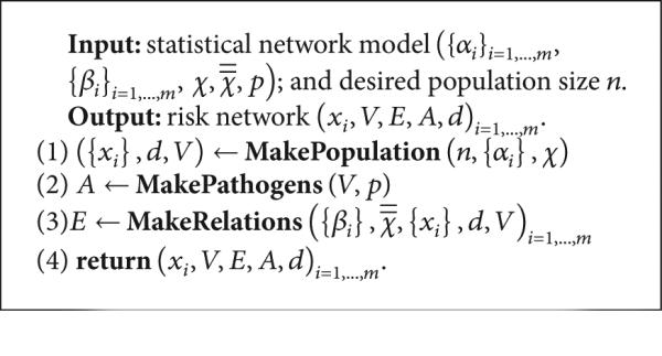
Procedure MakeNetwork.

Listing 2.

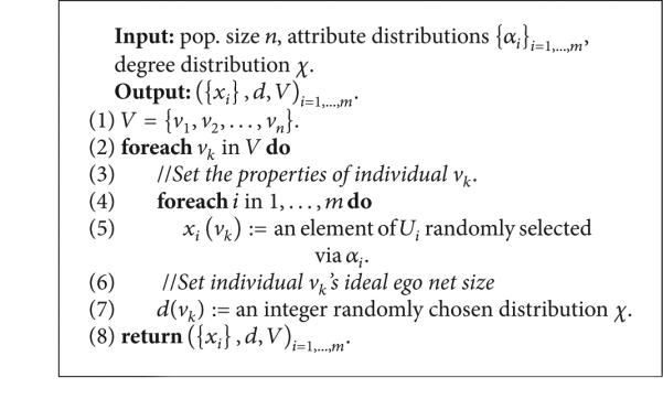
Procedure MakePopulation.

Listing 3.

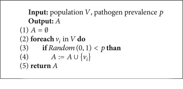
Procedure MakePathogens.

Listing 4.

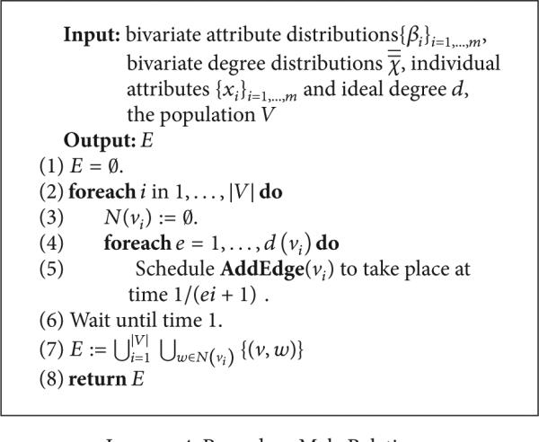
Procedure MakeRelations.

Each execution of AddEdge takes place in the context of a specific vertex ν, at a specific time t (Listing 5). Hereafter, all time-varying sets and functions (e.g., V, N) shall be so designated by providing the temporal coordinate t as superscript (i.e., as V^t , N^t). Procedure AddEdge determines the set of new neighbor candidates (line 2), consisting of vertices which are not already neighbors of ν. If candidates exist (line 3), the procedure computes the edge deficit for each candidate c (line 5) as the difference between c's ideal degree d(c) and actual degree |N^t(c)|, rescaling this into [0, 1] by composing with the smooth function e^−1/x that approaches 1 as x → ∞ and 0 as x → 0⁺ The quantity a_δ(c)is thus near 1 whenever |N_t(c)| < < d(c) and becomes 0 when c's actual degree |N^t(c)| attains its ideal value d(c). The selection of candidate d835dc50 is also influenced by the actual degrees of ν and c (line 6), reflecting the bivariate degree distribution $\overline{\overline{\chi }}$ (suitably binned to 2ε-sized buckets). Likewise, the joint attributes of ν and c influence the candidate selection (line 7), reflecting the bivariate attribute distributions β_i. These three factors are aggregated as c's propensity ω(c) (line 8), which is then normalized across C to define a probability distribution q (line 9). Finally, a candidate ω is selected from C (line 10) via the probability distribution d835dc5e just defined, and the edge (ν, ω) is added (line 12) by augmenting the neighbor set of ν.

Listing 5.

Procedure AddEdge.

To understand the three biases used in defining ω(c), we remark that taking ω(c) = a^t_X(c) would have made the probability of (ν, c) being selected proportional to the bivariate degree distribution $\overline{\overline{\chi }}$ evaluated in the neighborhood of ν and c's actual degrees. Using a^t_β(c) as a factor within the definition of ω(c) thus ensures that a pair of vertices (ν, c) that is exceptional with respect to $\overline{\overline{\chi }}$ will be correspondingly improbable as a candidate for the addition of an edge. Likewise, taking ω(c) = a^t_β(c) would have made the probability of (ν, c) being selected proportional to the product of the m bivariate attribute distributions β_i evaluated at ν and c. Using a^t_β(c) as a factor within the definition of ω(c) thus has the effect that a pair of vertices (ν, c) which are exceptional with respect to any β_i will be also be improbable as a candidate pair for the addition of an edge. Finally, the bias a_δ(c) favors the selection of candidates who still have a large residual degree (i.e., deficit from ideal degree). Over the course of the network building process, this bias has the effect of ensuring that all nodes in the network have residual degrees of comparable magnitude. By ensuring that all nodes maintain comparable residual degrees, we minimize the chances that the network building process will “get stuck” (i.e., reach a state in which the subset of nodes having positive residual degree already form a clique in the network built so far). While it is true that these three biases a_δ(c), a^t_X(c), and a^t_β(c) could have been aggregated to form ω(c) in a variety of ways, we chose to use their product in order to ensure that a candidate that is very improbable with respect to any one (or more) of the constituent factors will be rendered unlikely to be selected. More sophisticated definitions of ω (e.g., where the constituent factors a_δ(c),a^t_X(c), and a^t_β(c) are each exponentiated by different constants to allow for differences in their relative influence) were considered, but the experimental outcomes we report on here were found to be robust to a wide range of exponent values, and so the simple product formulation was deemed adequate for this exposition.

2.2. Network Dynamism Model

Individual agency may drive PWIDs to leave the risk network over time. To model this, each node ν is assigned a network lifetime L(ν) when it first enters the network, chosen by sampling from a positive truncated Gaussian [25] of mean μ^st and standard deviation σ^st . In the context of this work, a dearth of hard diachronic data forced us to choose μ^st and σ^st based on the ethnographic reports of researchers in the SFHR study. We took μ^st = 60, σ^st = 48 months, reflecting reports that PWIDs in the SFHR network remained participants for a period ranging between 2 and 8 years.

Whenever the network lifetime L(ν) of node ν expires, it breaks its risk relationships and removes itself from the network. The proposed network dynamism model assumes a constant population size |V^t| = |V¹| (for t > 1); so the departing individual ν is immediately replaced with a new individual ν′ . The attributes x_i(ν′) are determined by α_i and the ideal degree d(ν′) by X, in much the same manner as when the initial population was sampled (see lines new 4–6 of Listing 2).

The individual ν′ connects to d(ν′) existing nodes in the network by repeatedly calling a modified version of AddEdge in which the bias due to degree constraints has been modified (compare with line 5 of Listing 2) as follows:

$$a_{\delta }\left(c\right)≔\frac{{((\mid N^t\left(c\right)\mid +1)∕(d\left(c\right)+1))}^{w^S}}{{((\mid N^t\left(c\right)\mid +1)∕(d\left(c\right)+1))}^{w^S}+1}.$$ (7)

Note that a_δ(c) = 1/2 whenever |N^t(c| = d(c), and that

$$\begin{array}{cc}\hfill & \frac{d\left(c\right)}{\mid N^t\left(c\right)\mid }\to \infty \Rightarrow a_{\delta }\left(c\right)\to 1,\hfill \\ \hfill & \frac{d\left(c\right)}{\mid N^t\left(c\right)\mid }\to 0^{+}\Rightarrow a_{\delta }\left(c\right)\to 0.\hfill \end{array}$$ (8)

The parameter W^S controls the rate at which a_δ(c) approaches the limits asserted above and so determines how closely individual nodes adhere to their ideal degree over the course of their network lifetimes. Justification for an individual having an intrinsic ideal degree comes from prior work on network “roles” and the correlations between role and ego network size [9, 24]. In the context of this work, we took W^S = 2.9, thereby ensuring that when actual degree was more than 30% above ideal degree a_δ(c) ≈ 0 (and analogously, when actual degree was more than 30% below ideal degree, a_δ(c) ≈ 1).

2.3. Infection Model

Each individual ν in the network has an intrinsic tendency to engage in risk acts t^R(ν), which is assumed to be time-invariant and drawn at the outset from the positive reals using a truncated Gaussian [25] with mean μ^R and standard deviation σ^R. In the course of simulations, a risk event stream is generated at each individual ν as a Poisson process wherein the time between successive impulses follows an exponential distribution having rate |N^t(ν)|/t^R(ν). Upon experiencing a risk event at time t, node ν selects a partner W uniformly at random from among its neighbors N^t(ν) and engages in a mutual risk act with W.

In the context of this work, μ^R and σ^R were set in accordance with the SFHR data set. Given that the criterion for a “link” in the SFHR survey was “participation in a mutual risk act in the last 30 days” [26, page 115], the parameter μ_R was set to 1.0 months, so that nodes would draw from a distribution of risk profiles centered at 1 risk event per month per risk partner. Given that the mean degree of nodes in the SFHR network was 3.4, the actors in our model would, on average, engage in 3-4 risk events per 30-day period. This aligns well with the 30-day risk event rate analyses in the study report [26, page 136-7]. SFHR interview subjects reported an average of 112 monthly injections with a standard deviation of 139 [26, page 120]. Taking these numbers as our guide, we set the standard deviation for the risk distribution σ_R to be equal to the mean β_R. This produced a distribution for t^R that was near-uniform between 0 and 2, with a long but rapidly diminishing tail for rates greater than 2 risk events per number of risk partners per month.

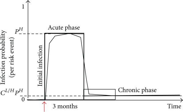
During each risk act, the likelihood of viral transmission is 0 if both individuals have the same infection status. If the individuals are serodiscordant (i.e., precisely one of them is infected), then the probability of transmission is modeled by an infectiousness curve I⁺ which maps the age of the infection (amount of time that has elapsed since the positive individual in the pair first became infected) to the probability of the pathogen's transmission. In the case of HIV, the infectiousness curve decreases sharply at approximately three months and remains at very low levels until over eight years later [27–29]. Given that HIV infectiousness drops sharply approximately 3 months after the time of initial infection, we model I⁺ as a two-parameter step function (see Figure 1) whose value is p^H for the 3-month acute phase and C^L/H · p^H in the subsequent chronic phase (c^L/H < < 1).

Figure 1.

A two-parameter representation of HIV infectiousness as a function of infection age.

In the context of this work, p^H and c^L/H were set in accordance with prior knowledge concerning HIV. While no precise data was available on per-risk-event infection probability for HIV, Hagan and colleagues found that HCV risk among PWID showed a 3- to 5-fold increase in sero-conversion rates and a risk factor of 5.9 for those who shared drug preparation equipment or syringes [30]. Initially, p^H was to be a tuning parameter such that once all other parameters had been set according to the SFHR data, a series of trials could be undertaken in simulated networks and dp^H set to yield HIV prevalence stabilization levels that matched those observed historically in the SFHR network (i.e., 40%–50%). This proved unnecessarily sophisticated, as variations in the per-risk-event infection probability (from as low as 2% to as high as 10%) showed little effect on HIV prevalence stabilization levels. In the end, we chose a per-risk-event infection probability p^H = 5%. The value of c^L/H was taken to be 1/100, a representative value in the range of published estimates (between 1/20 and 1/1000) for relative HIV infectiousness in the chronic versus acute phase [28, 31].

3. Measuring Firewalling Effects

At a time t, two types of network obstructions curtail the continued growth of the set of HIV+ individuals $A^t\subseteq V^t$ in a risk network G^t = (V^t, E^t):

(i) Type 1. The risk network G^t may not be a connected graph. Since the virus propagates over risk relationships, the multiplicity of components may act as a network obstruction to viral propagation.

(ii) Type 2. An HIV– individual whose viral burden is in the chronic low-infectiousness phase cannot be reinfected through new risk behaviors, and so cannot return to a state of acute infectiousness. When such an individual separates HIV– nodes from acute HIV+ individuals, it obstructs the transmission of the virus from the latter to the former.

In this section, we formally define a graph-theoretic measure which captures the extent to which HIV– individuals can attribute their uninfected status to the two types of network obstructions described above.

Towards this, let ${\widehat{G}}^t$ be the graph obtained by deleting from G^t all infected individuals in the chronic phase along with all their incident edges. The individuals in the chronic phase are precise:

$$O^t\stackrel{\mathrm{def}}{=}\{v\mid I^{+}\left(v\right)\le c^{L∕H}\cdot p^H\}\subseteq A^t,$$ (9)

and since the virus cannot re-infect individuals in O^t, the graph ${\widehat{G}}^t$ may be thought of as the virus's view of the network G^t. While the graph ${\widehat{G}}^t$ need not be connected, it may be (uniquely) decomposed into maximal connected components:

$${\widehat{G}}^t={\Gamma }_1^t\bigsqcup {\Gamma }_2^t\bigsqcup \cdots \bigsqcup {\Gamma }_{{\ell }^t}^t.$$ (10)

We introduce an indexing function $i^t:V^t=O^t\to \{1,\dots ,{\ell }^t\}$ to identify the component in which each individual ν in VtOt may be found; that is, $i^t\left(v\right)=j\iff v\in \Gamma j^t$. We are interested in the situation where an HIV– individual V lies in a component of ${\widehat{G}}^t$ that contains one of the known acute HIV infections:

$$H^t\stackrel{\mathrm{def}}{=}\{v\mid I^{+}\left(v\right)\ge p^H\}\subseteq A^t,$$ (11)

since this implies that ν may potentially acquire the virus through a sequence of one or more transmissions. Accordingly, we define a Boolean-valued function ϕ^t : V^t \ A^t →{0, 1} by putting

$${\varphi }_t\left(v\right)\stackrel{\mathrm{def}}{=}\{\begin{array}{cc}1\hfill & {\Gamma }_{i^t\left(v\right)}^t\cap H^t=\varnothing ,\hfill \\ 0\hfill & \text{otherwise}.\hfill \end{array}\phantom{\}}$$ (12)

Now, ϕ^t(ν) = 1 if and only if V is in a component of ${\widehat{G}}^t$ with no acute infections. Pulling back from the virus' viewpoint ${\widehat{G}}^t$ to the human perspective G^t, we see that ϕ^t(ν) = 1 if either (1) ν is in a component of G^t with no acute infections or (2) ν is in a component of G^t containing acute infections but all paths from ν to acute HIV+ individuals are blocked by interceding chronic HIV+ individuals. It follows that ϕ^t(ν) = 1 precisely when an HIV− individual ν is enjoying one of the two types of network obstructions presented at the outset of this section. We now introduce the quantitative measure:

$$\mathrm{FW}\left(t\right)\stackrel{\mathrm{def}}{=}\frac{{\sum }_{v\in V^t=A^t}{\varphi }^t\left(v\right)}{\mid V^t=A^t\mid }.$$ (13)

When FW(t) ≈ 1, almost all HIV− individuals are experiencing one of the two types of network obstructions described above; when FW(t) ≈ 0, the two types of network obstructions cannot be said to significantly account for the HIV− status of the uninfected individuals.

3.1. An Example

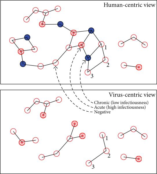
The top image in Figure 2 shows a 26-node risk network with three connected components consisting of 2, 3, and 21 individuals. The bottom image shows the corresponding 6-component risk network obtained once individuals with chronic-phase infections (blue nodes) and their incident edges have been deleted. In effect, the top figure is a human-centric rendering of the risk network, while the combinatorial object at the bottom is a virus-centric rendering of the same risk network. At each instant in time, the virus-centric rendering of risk network may be decomposed into a collection of connected components. The fates of individuals in each connected component therein are seemingly intertwined by sequences of risk relationships, while individuals lying in different components have more independent destinies with respect to infection outcomes (assuming the instantaneous network structure). Each connected component can be assigned a risk status, wherein it is deemed to be at risk (resp., firewalled) if acute infections (red nodes) are present (resp., absent) from it. In the virus-centric rendering of the risk network shown at the bottom of Figure 2, there are 4 components at risk and 2 which are firewalled. In this analysis, the uninfected individuals within each component in the virus-centric view inherit the risk status of the component in which they lie. Since the 4 components that are at risk have 4, 2, 3, and 1 uninfected individuals in them respectively, the total number of individuals said to be at risk is 4 + 2 + 3 + 1 = 10. On the other hand, since the 2 components that are firewalled both have 3 uninfected individuals in them, the total number of individuals said to be firewalled is 3 + 3 = 6. From this, we conclude that out of the total 10 + 6 = 16 uninfected individuals, a 6/16 = 0.375 fraction may attribute their present good fortune to the fact that the virus cannot reach them because of the network partitioning induced by old infections and/or link sparsity. In the example, the value of the FW measure is 0.375, which is a relatively low value within the range 0 to 1 of possible values.

Figure 2.

(Top) Risk network with 10 HIV+ (4 acute) out of 26 nodes; (bottom) virus-centric view, FW: 6/16 = 0.375.

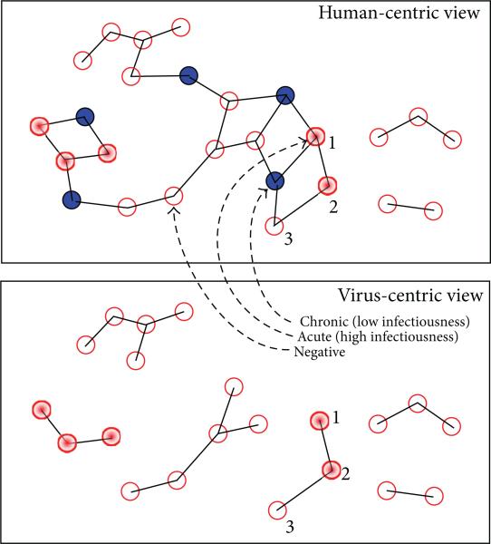
Now consider the human-centric view of a topologically isomorphic risk network shown at the top of Figure 3, having precisely the same pathogen prevalence, and the same number of acute and chronic infections as the previous network considered in Figure 2. Since the chronic infections are situated identically in the two networks, the virus-centric views are isomorphic (as graphs). What is different between the two networks, however, is the placement of acute infections (relative to the constant locations of chronic infections). The virus-centric view of the network in Figure 3 has 2 at-risk components and 4 firewalled components. Of the 16 uninfected individuals, the number that is at risk is 1, while the number that is firewalled is 15. Thus, the value of the FW measure is 15/16 = 0.938, a relatively high value within the range 0 to 1 of possible values. What these two examples illustrate is that the FW measure is defined in terms of the local network structure relevant to the virus propagation dynamics and depends heavily on the relative placement of acute and chronic infections within the risk network.

Figure 3.

(Top) Risk network with 10 HIV+ (4 acute) out of 26 nodes; (bottom) virus-centric view, FW: 15/16 = 0.9375.

4. Simulation Experiments

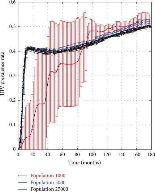
In this section, we use the SFHR-based statistical network model (with a modified pathogen prevalence parameter p = 0.001) to sample artificial risk networks of 1000–25,000 nodes containing 0.1% HIV+ individuals. These artificial networks serve as initial states of a stochastic discrete dynamical system whose evolution is governed by the dynamism and infection models of Sections 2.2 and 2.3. We simulated multiple 15-year trajectories of the system and computed the HIV prevalence rates along these trajectories as functions of time. Figure 4 shows that HIV prevalence stabilized at approximately 40% in all but the 1000-node network. Each graph shows the results obtained across 10 simulation trials, with vertical bars indicating the standard deviations. To give the reader a sense of scale, in a 25,000 node network, each trial entailed that approximately 15.5 million risk events across which HIV infection could have taken place.

Figure 4.

HIV rates in PWID networks of size 1 k–25 k nodes.

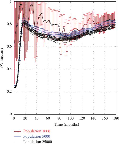
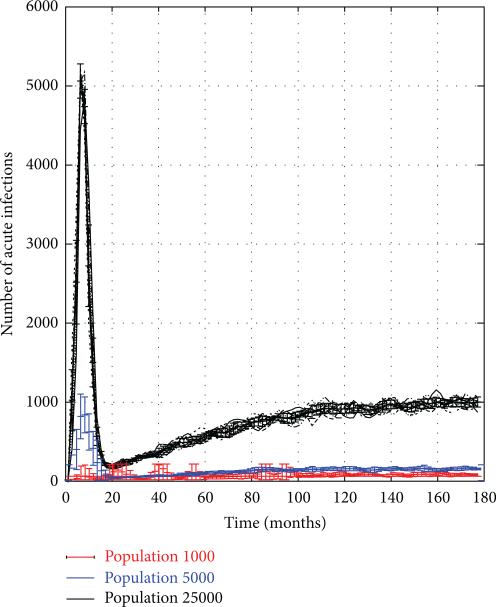
To test the firewall hypothesis, the system was frozen in mid-trajectory at monthly time intervals so the value of the FW measure could be computed (as defined in (13)). Figure 5 depicts the value of FW(t), plotted as a function of time t for 15-year trajectories corresponding to the same set of trials shown in Figure 4. We see that the FW measure rises rapidly from 0 to 0.8 during the first 18 months, rebounding briefly to 0.75 in the next 5 years, and then restabilizing again back at the 0.8 level. Despite the fact that the 1000-node network showed high variation in the HIV prevalence between different trials, and a much more gradual rise in overall rates, here too the firewall hypothesis seems to hold true, though there are greater variations across trials. While the graphs show that 70–80% of HIV− individuals were firewalled, this does not imply that new, acute (and thus highly infectious) HIV infections did not occur. Rather, as seen in Figure 6, acute infections continued to appear in the network at a relatively steady rate even after the initial hot spike, though clearly they failed to propagate across the network.

Figure 5.

Firewall Hypothesis Validity in PWID networks of size 1 k–25 k nodes.

Figure 6.

Number of acute HIV infections in PWID networks of size 1 k–25 k nodes.

5. The Emergence and Maintenance of Firewalls

To facilitate further analysis, we divided the trajectories, referring to the first 18 months as the emergent period, and the 13+ later years as the steady period. Each of the periods is treated in turn in the sections that follow.

5.1. Emergent Period

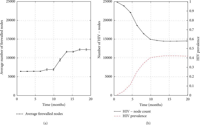
To understand the behavior of the FW measure along system trajectories, we return to its definition as the quotient of the number of firewalled individuals by the number of HIV− individuals. The number of firewalled individuals in a risk network of 25,000 nodes is depicted over the 18-month emergent period in the left graph in Figure 7. We can see from the graph that at the outset, approximately 25% of all individuals are firewalled, but that this number doubles and plateaus over the 18-month duration of the emergent period. A closer examination reveals that the initial value of the FW measure is attributable to Type 1 network obstructions, while its subsequent rise (to be considered in detail) is due to the emergence of Type 2 obstructions. The number of HIV− individuals, on the other hand, can be readily determined from HIV prevalence levels. The right graph of Figure 7 shows that over 18 months, the number of HIV negative individuals falls from its initial value of 99.5% of all individuals, plateauing at a mere 57%, just one year into the simulation. To obtain a clearer understanding of “why” these two ingredient quantities behave as they do, we shall make use of the two graphs in Figure 8 which present an array of measure (means) derived from 10 simulation trials of 25,000 node networks.

Figure 7.

The emergent period: (a) firewalled nodes; (b) HIV prevalence, number of HIV− individuals.

Figure 8.

The firewall effect during the emergent period.

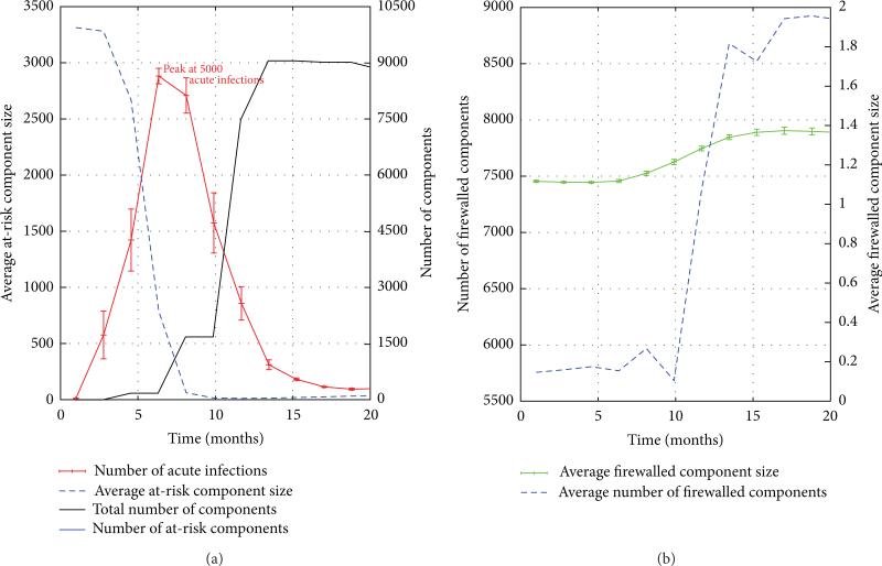
(a) The Number of HIV− Individuals. Figure 8(a) reveals that the number of acute HIV infections rises exponentially from close to 0 to around 5,000 over a brief 6-month initial segment of the emergent period. after that, the number of acute infections begins to decline. To understand why this occurs, we observe that the average size of at-risk components decreases sharply from over 3,000 to nearly 1 by month 7 of the emergent period (see Figure 8(b)). As the average at-risk component size becomes smaller, each acute infection can impact very few HIV− individuals through transmission. When the ability of acute infections to spread has been mitigated in this way, as it clearly has by month 7, acute infections cease to be able to increase exponentially, and instead begin to decay in number as they transition from acute to chronic phase over time. This explanation is confirmed (Figure 8(a)) by the drop in the number of acute infections beginning at month 7 of the simulation. Note that the number of acute infections does not drop to 0 because even chronic infections have a nonzero probability (c^L/H·p^H > 0) of transmitting HIV and thereby generating new infections. Thus, we see that the large numbers of chronic infections act as a reservoir of infectiousness and are responsible for continuing to produce new infections that fail to propagate fully throughout the network. This decline in the number of acute infections (beginning in month 7) explains the corresponding leveling off in the number of HIV− individuals (see the right graph in Figure 7).

(b) The Number of Firewalled Nodes. We begin by considering Figure 8(a), noting that three months after the hot spike in acute HIV infections begins (i.e., as acute infections start to transition into the chronic phase), the number of components (in the virus-centric view of the risk network) begins to rise, causing individuals to be removed from the virus-centric view and splitting the risk network into many components in the process. The increase in number of components (from 5,700 to 9,000) takes longer than the increase in the number acute infections because not every transition of an HIV+ individual from acute to chronic phase induces a partition in the virus-centric risk network. It is natural to ask whether the 3,300 new components that arise are predominantly fire-walled or at-risk? To resolve this, we note that the number of at risk components, shown in the lower left graph, declines dramatically at this time, ending in month 20 at a level of 500. Even if all 500 of these at-risk components were to be found among the 3300 new components created over the emergent phase (and thus none were the result of a low probability infection from a nonacute HIV+ individuals), this would still indicate that a majority of the new components created between month 10 and month 20 would be classified as firewalled. Since many new firewalled components of roughly constant size are being created (see Figure 8(b)), we expect the number of firewalled nodes to grow and taper, mirroring the growth curve of the number of components.

5.2. Steady Period

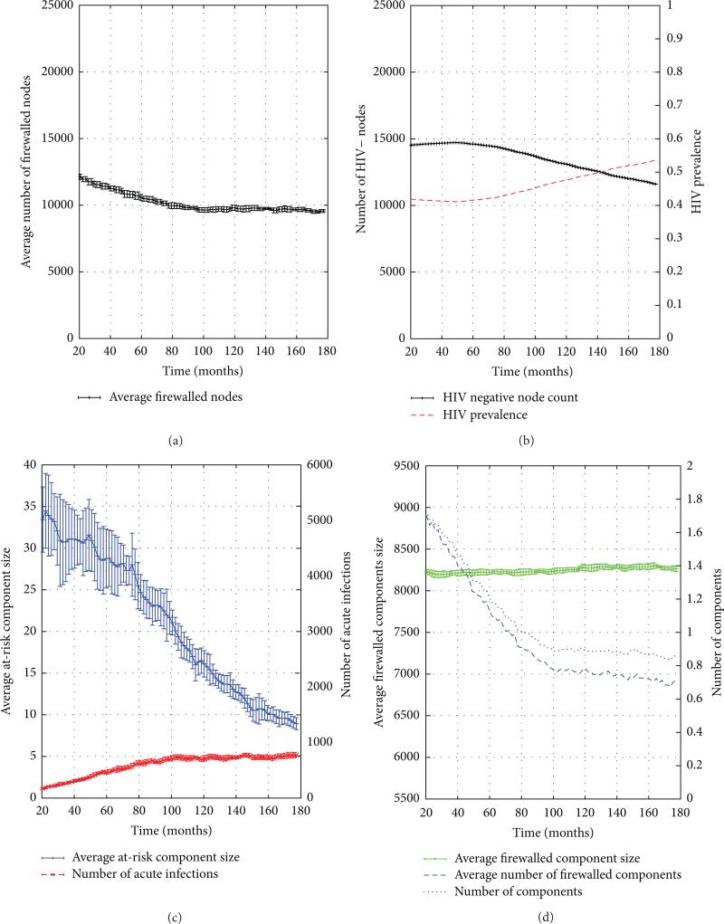
As in our consideration of the emergent phase, the graphs discussed here are drawn from 10 trials of 25,000-node PWID networks drawn from the statistical network model extracted from the SFHR data set. We now consider the dynamics of the FW measure's numerator and denominator during the steady period, after the hot spike in new infections has subsided. During the steady period, the number of firewalled individuals (numerator) is seen to decline from 12,000 to 10,000 over the 13+ years of the simulation (see Figure 9(a)). The number of HIV− individuals (denominator) is seen to slowly decrease from just under 15,000 to just under 12,000 over the same time period (see Figure 9(b)). To render transparent the mechanisms underlying this behavior, we shall make use of the bottom two auxiliary graphs in Figure 9.

Figure 9.

The firewall effect during the steady period.

(a) The Number of HIV− Individuals. Figure 9(c) depicts both the number of acute infections and the average risk component size over time. In our base SFHR model c^L/H · p^H = 0.05 × 0.01 = 5 · 10^–4, which while being small is still nonzero, providing a slow burn that continuously produces new infections but is unable to explode into a hot spike because the average at-risk component size is small (thanks to the previously demonstrated structural side effects of the emergent phase), going from a mean size of nearly 35 nodes down to a less than 10 over the 160 months of the steady period. The slow burn proceeds, driving the mean size of at-risk components lower, which in turn, limits the extent to which new acute infections can spread. The result is that these two quantities (number of acute infections and average risk component size) equilibrate over the steady period. Given an understanding of the trajectory of acute infections, we implicitly arrived at an explanation of the trajectory of the number of HIV− individuals, since these two quantities are trivially related (Figure 9(b)): if the number of acute infections stabilizes to a constant nonzero number, then HIV prevalence will increase at a rate proportional to this number.

(b) The Number of Firewalled Nodes. We turn our attention now to the number of firewalled nodes (Figure 9(a)). Figure 9(d) shows that in the first 5 years of the steady period, the total number of components (in the virus-centric view of the risk network) declines from 9,000 components to 7,200, or roughly 80% of its starting value. This implies that 1,800 components seemingly vanished, and it is natural to ask, as before, whether these 1,800 components were predominantly of the firewalled or at-risk classification? The graph shows us that the number of firewalled components experiences a commensurate decline—and hence the components being destroyed in the first 5 years are in fact almost exclusively fire-walled components. How might this happen? The third curve in the graph shows the average size of firewalled components over time. We see that this number stays fairly steady in the neighborhood of 1.4, implying that a significant number of the firewalled components are islets. It is now apparent what is occurring: when firewalled islets become infected by the slow burn of adjacent old infections, firewalled components disappear from the virus-centric network.

5.3. Robustness Considerations. Having conducted simulation experiments based on the SFHR model and used these to demonstrate the occurrence of subsaturation stabilization via the firewall hypothesis, we acknowledge that the model contains a large number of parameters. While these parameters were set to consensus estimates derived from the ethno-graphic data collected as part of the SFHR study, it would be natural to ask whether the parameter settings had a significant impact on the emergence of subsaturation stabilization and the firewall phenomena in the above experiments. Significant model parameters included the following:

(1) from Section 2.1(c), the univariate attribute distributions α₁, α₃, and α₃, the bivariate attribute distributions β₁, β₂, and β₃, and the univariate (resp., bivariate) degree distributions χ (resp., $\overline{\overline{\chi }}$) together reflect statistical properties of the network edges. To evaluate the impact of these parameters, we repeated the previously described experiments using a statistical network model derived from Project 90 (P90), another PWID risk network study. Conducted between 1988 and 1992 in Colorado Springs, P90 was a prospective study of heterosexual subjects who were defined as being at “high risk” for STI/HIV infection [32, 33]. Eligible subjects reported at least one of the following behaviors in the past 12 months: exchanging sex for money or drugs, sex (paying or nonpaying) with a prostitute, injection of illicit drugs, or sex with an injection drug user. Unlike the cross-sectional SFHR, the P90 study followed its subjects for up to 5 years, with no requirement for year-to-year continuity; new subjects were additionally recruited each year. 595 enrolled individuals produced 1091 interviews, which named 8,164 network contacts overall [32, 34–39]. The P90-based simulations were designed to overlap in scale with the SFHR-based simulations described above. We found that the specific topology of the real-world network from which the statistical network model is derived plays a minor role (a few percentage points) in the stabilization level dynamics and the FW measures manifested. In particular, analogous subsaturation stabilization and firewall effects are apparent in simulations based on the model derived from the P90 study.

(2) From Section 2.2, the parameters μ^st, σ^st serve to specify the process by which individuals depart from and arrive at the network, while ω^S regulates node adherence to ideal degree. To evaluate the impact of μ^st, σ^st, we simulated networks based on the SFHR model in which μ^st (mean duration of in-network lifetime in months) was artificially set to half (resp., double) its estimated value, that is, 30 (resp., 120) months. In these simulations, we found that HIV rates stabilized to subsaturation levels within 5% of those manifested in the “standard” SFHR experiments. The firewall effect continued to be manifested, though the value of the FW measure was approximately 10% lower (resp., 10% higher) than what was seen in “standard” SFHR experiments. To evaluate the impact of ω^S, we simulated networks based on the SFHR model in which ω^S was artificially set to half (resp., double) its estimated value, that is, 1.5 (resp., 6). In these simulations, we found that HIV stabilization (resp., the firewall effect) continued to be apparent, with prevalence levels (resp., FW measure) deviating by less than 5% relative to the values observed in the “standard” SFHR experiments.

(3) From Section 2.3, the parameters μ^R, σ^R serve to specify the random process determining each individual's risk acts, while p^H, c^L/H govern the form of the HIV infectiousness curve I+. To evaluate the impact of μ^R, σ^R, we simulated networks based on the SFHR model in which μ^R (mean time between risk impulses in months) was artificially set to half (resp., double) its estimated value, that is, 0.5 (resp., 2) months. In these simulations, we found that HIV rates stabilized to subsaturation levels approximately 40% higher (resp., 30% lower) than those manifested in the “standard” SFHR experiments. The firewall effect continued to be manifested, though the value of the FW measure was approximately 20% higher (resp., 30% lower) than in the “standard” SFHR experiments. To evaluate the impact of p^H, c^L/H we simulated networks based on the SFHR model in which the parameter p^H (transmission probability during acute period) was artificially set to half (resp., double) its estimated value, that is, 2.5% (resp., 10%). In these simulations, we found that HIV rates stabilized to subsaturation levels approximately 50% lower (resp., 30% higher) than those manifested in the “standard” SFHR experiments. The firewall effect continued to be manifested, though the value of the FW measure was approximately 40% lower (resp., 20% higher) than in the “standard” SFHR experiments.

In summary, our conclusions concerning the emergence of subsaturation stabilization and the firewall phenomena (which were drawn from simulations parameterized by data from the SFHR study), are in fact robust within a wider range of model parameter settings, though the extent of the two phenomena (as evaluated by stabilized HIV prevalence levels and FW measure values) is certainly nominally influenced by the specific choice of model parameter settings.

6. Conclusions

Having described a stochastic dynamical system modeling a dynamic PWID risk network, whose simulated trajectories match the historical HIV dynamics known for PWID networks in New York City during the early 1980s, we determine that nodes with mature HIV+ status tend to divide the network into clusters of uninfected nodes that remained relatively stable over time. Thus, the FH holds significantly (for up to 80% of uninfected individuals) and so captures an important barrier to HIV propagation in PWID risk networks. In considering the microlevel mechanics underlying the emergence of the FH, we find it helpful to examine the network during two phases of HIV infection: an initial, emergent phase of rapid spreading and a later period of stable HIV rates. There is an enduring presence of new infections that fail to propagate during the stable phase, and this is because of the structural effects created during the emergent phase when a significant fraction of uninfected nodes coalesce into small components (in the virus-centric view of the network). These small clusters represent margins of the network and are often composed of a few (or even single) individuals. Small components ensure that the ability for new infections to spread across the network via such individuals is near nil, even when new infections occur and individuals enter into a period of high infectiousness, and even as members of the network continue to engage in risk events that can transmit the virus.

Our research also suggests that overall network size plays a key role in HIV dynamics among injecting drug user networks. Consistently, networks of size 5,000 through 25,000 behaved within a narrow (and therefore predictable) range of overall characteristics. Networks of 1000 nodes or fewer, on the other hand, showed high variability in their network-wide behavior. This latter finding bears serious consideration for those concerned with interventions aimed at influencing the overall rate of HIV among injecting drug user networks. If smaller networks show high variability in their dynamics— leading to the idea that they are more subject to stochastic events than networks of large size—then understanding where and how particular interventions will succeed or fail becomes very difficult. What such variability in outcomes indicates is that stochastic factors may outweigh node level dynamics in determining network-wide outcomes through time in small networks. Put another way, the outcome of interventions in small-scale networks may not serve as good indicators of likely outcomes of the same intervention in other small networks, nor in the same networks at a different time, nor in large networks. In each case, the effects of random events may render the otherwise most successful interventions moot, or the most ill-adapted interventions successful—this without a change in the underlying set of network attributes or dynamics. We recognize that this finding represents a difficult challenge to policies advocating demonstrated evidence-based interventions (DEBIs) [40]. Regardless of whether the precise findings regarding scale seen here hold up under further investigation, it is clear that factors of scale ought to be an important criterion for evaluating what constitutes “demonstration” in evaluating intervention success or failure.

Simulation of formal dynamical systems is far from demonstration of actual disease dynamics, of course. But the results of this project can point to ways that network wide phenomena are shaped by local social processes, and thereby open avenues for future research that may be hidden by the limits of more standard empirical investigation. We note that the disease dynamics reflected here may be partly explained by the social circumstances that produce the SFHR PWID risk network (on which the simulation topologies were based). Among the most important of these is the central role that shooting galleries played as venues for drug use at the time of the SFHR study [6, 14, 24, 41]. These and other forms of enforced propinquity were encouraged by significant changes in drug enforcement regimes in New York at the time. During the 1991–93 time frame, New York City as a whole—and Bushwick in particular, where much of the SFHR study was conducted—was undergoing a change in drug interdiction regimes aimed at closing down “open air” drug markets and injection locations [42–45]. This strategy involved broad “sweeps” in which outdoor users were routinely arrested for small amounts of drug possession. As places serving as outdoor drug use locations were increasingly systematically pursued by law enforcement, outdoor drug use became increasingly precarious, and indoor, more discreet drug use locations (shooting galleries) grew in importance as a result [44].

These circumstances may have, at least initially, helped promote the firewall effect described here. Under such conditions, new users with few network connections are likely to find themselves in shooting galleries with shooting gallery operators who were both of high degree and more likely to be in a state of mature infection, and thus effective fire-walls against new infections potentially moving through the network. Conversely, as police interdiction gradually came to target shooting galleries (and shooting gallery operators became targets of police arrest), the disruption of stable relationships and the removal of critical central nodes from the network may disrupt this firewall effect, forcing remaining network members to seek out new sources and injection partners. This would have the effect of significantly reorganizing the network (in the virus-centered view). Police decisions were obviously weighted by other concerns, but an important suggestion of the simulation results presented here is that the public health implications of those decisions are likely difficult to gauge. Drug interdiction strategies are seldom seen as increasing risk, and it would likely seem highly counterintuitive that the removal of HIV+ individuals who have been infected for more than three months and who play a brokerage role in the network may in fact raise the level of risk for the remaining risk network—but that is what is suggested here. Such conclusions are obviously highly speculative. But they come as the results of models and simulations whose scale and scope cannot be matched by more direct empirical research. It remains before us to translate these suggestions into concrete research strategies capable of testing and evaluating both these results and their implications for public policy.

References

- 1.Bachanas PJ, Morris MK, Lewis-Gess JK, et al. Predictors of risky sexual behavior in African American adolescent girls: implications for prevention interventions. Journal of Pediatric Psychology. 2002;27(6):519–530. doi: 10.1093/jpepsy/27.6.519. [DOI] [PubMed] [Google Scholar]
- 2.Friedman SR, Neaigus A, Jose B, et al. Sociometric risk networks and risk for HIV infection. American Journal of Public Health. 1997;87(8):1289–1296. doi: 10.2105/ajph.87.8.1289. [DOI] [PMC free article] [PubMed] [Google Scholar]
- 3.Bell DC, Montoya ID, Atkinson JS, Yang SJ. Social networks and forecasting the spread of HIV infection. Journal of Acquired Immune Deficiency Syndromes. 2002;31(2):218– 229. doi: 10.1097/00126334-200210010-00013. [DOI] [PubMed] [Google Scholar]
- 4.Goodreau SM. Assessing the effects of human mixing patterns on human immunodeficiency virus-1 interhost phylogenetics through social network simulation. Genetics. 2006;172(4):2033–2045. doi: 10.1534/genetics.103.024612. [DOI] [PMC free article] [PubMed] [Google Scholar]
- 5.Des Jarlais DC, Arasteh K, Friedman SR. HIV among drug users at beth israel medical center, new york city, the first 25 years. Substance Use and Misuse. 2011;46(2-3):131–139. doi: 10.3109/10826084.2011.521456. [DOI] [PubMed] [Google Scholar]
- 6.Friedman SR, Curtis R, Neaigus A, Jose B, Jarlais DCD. Social Networks, Drug Injectors’ Lives, and HIV/AIDS. 1st edition Springer; 2010. [Google Scholar]
- 7.Friedman SR, Kottiri BJ, Neaigus A, Curtis R, Vermund SH, Des Jarlais DC. Network-related mechanisms may help explain long-term HIV-1 seroprevalence levels that remain high but do not approach population-group saturation. American Journal of Epidemiology. 2000;152(10):913–922. doi: 10.1093/aje/152.10.913. [DOI] [PubMed] [Google Scholar]
- 8.Des Jarlais DC, Perlis T, Friedman SR, et al. Declining seroprevalence in a very large HIV epidemic: injecting drug users in New York City, 1991 to 1996. American Journal of Public Health. 1998;88(12):1801–1806. doi: 10.2105/ajph.88.12.1801. [DOI] [PMC free article] [PubMed] [Google Scholar]
- 9.Friedman SR, Furst RT, Jose B, et al. Drug scene roles and HIV risk. Addiction. 1998;93(9):1403–1416. doi: 10.1046/j.1360-0443.1998.939140311.x. [DOI] [PubMed] [Google Scholar]
- 10.Friedman SR, Mateu-Gelabert P, Curtis R, et al. Social capital or networks, negotiations, and norms? A Neighborhood Case Study. American Journal of Preventive Medicine. 2007;32(6):S160–S170. doi: 10.1016/j.amepre.2007.02.005. [DOI] [PMC free article] [PubMed] [Google Scholar]
- 11.Goldstein MF, Friedman SR, Neaigus A, Jose B, Ildefonso G, Curtis R. Self-reports of HIV risk behavior by injecting drug users: are they reliable? Addiction. 1995;90(8):1097–1104. doi: 10.1046/j.1360-0443.1995.90810978.x. [DOI] [PubMed] [Google Scholar]
- 12.Jose B, Friedman SR, Neaigus A, et al. Syringe-mediated drug-sharing (backloading): a new risk factor for HIV among injecting drug users. AIDS. 1993;7(12):1653–1660. doi: 10.1097/00002030-199312000-00017. [DOI] [PubMed] [Google Scholar]
- 13.Kottiri BJ, Friedman SR, Neaigus A, Curtis R, Des Jarlais DC. Risk networks and racial/ethnic differences in the prevalence of HIV infection among injection drug users. Journal of Acquired Immune Deficiency Syndromes. 2002;30(1):95–104. doi: 10.1097/00042560-200205010-00013. [DOI] [PubMed] [Google Scholar]
- 14.Neaigus A, Friedman SR, Curtis R, et al. The relevance of drug injectors’ social and risk networks for understanding and preventing HIV infection. Social Science and Medicine. 1994;38(1):67–78. doi: 10.1016/0277-9536(94)90301-8. [DOI] [PubMed] [Google Scholar]
- 15.Neaigus A, Friedman SR, Goldstein M, Ildefonso G, Curtis R, Jose B. Using dyadic data for a network analysis of HIV infection and risk behaviors among injecting drug users. NIDA Research Monograph Series. 1995;151:20–37. [PubMed] [Google Scholar]
- 16.Bearman PS, Moody J, Stovel K. Chains of affection: the structure of adolescent romantic and sexual networks. American Journal of Sociology. 2004;110(1):44–91. [Google Scholar]
- 17.Frank O, Strauss D. Markov graphs. Journal of the American Statistical Association. 1986;81(395):832–842. [Google Scholar]
- 18.Holland PW, Leinhardt S. An exponential family of probability distributions for directed graphs. Journal of the American Statistical Association. 1981;76(373):33–50. [Google Scholar]
- 19.Snijders TAB, Pattison PE, Robins GL, Handcock MS. New specifications for exponential random graph models. Sociological Methodology. 2006;36(1):99–153. [Google Scholar]
- 20.Goodreau SM. Advances in exponential random graph (P*) models applied to a large social network. Social Networks. 2007;29(2):231–248. doi: 10.1016/j.socnet.2006.08.001. [DOI] [PMC free article] [PubMed] [Google Scholar]
- 21.Goodreau SM, Kitts JA, Morris M. Birds of a feather, or friend of a friend? Using exponential random graph models to investigate adolescent social networks. Demography. 2009;46(1):103–125. doi: 10.1353/dem.0.0045. [DOI] [PMC free article] [PubMed] [Google Scholar]
- 22.Kolaczyk ED. Statistical Analysis of Network Data: Methods and Models. 1st edition Springer; 2010. [Google Scholar]
- 23.Dombrowski K, Khan B, McLean K, et al. A re-examination of connectivity trends via exponential random graph modeling in two IDU risk networks. Substance Use and Misuse. 2012;49 doi: 10.3109/10826084.2013.796987. [DOI] [PMC free article] [PubMed] [Google Scholar]
- 24.Curtis R, Friedman SR, Neaigus A, Jose B, Goldstein M, Ildefonso G. Street-level drug markets: network structure and HIV risk. Social Networks. 1995;17(3-4):229–249. [Google Scholar]
- 25.Robert CP. Simulation of truncated normal variables. Statistics and Computing. 1995;5:121–125. [Google Scholar]
- 26.Friedman SR. Social Networks, Drug Injectors’ Lives, and HIV/AIDS. Springer; 1999. [Google Scholar]
- 27.Cates W, Chesney MA, Cohen MS. Primary HIV infection—a public health opportunity. American Journal of Public Health. 1997;87(12):1928–1930. doi: 10.2105/ajph.87.12.1928. [DOI] [PMC free article] [PubMed] [Google Scholar]
- 28.Kahn JO, Walker BD. Acute human immunodeficiency virus type 1 infection. The New England Journal of Medicine. 1998;339(1):33–39. doi: 10.1056/NEJM199807023390107. [DOI] [PubMed] [Google Scholar]
- 29.Lyles CM, Kay LS, Crepaz N, et al. Best-evidence interventions: findings from a systematic review of HIV behavioral interventions for US populations at high risk, 2000–2004. American Journal of Public Health. 2007;97(1):133–143. doi: 10.2105/AJPH.2005.076182. [DOI] [PMC free article] [PubMed] [Google Scholar]
- 30.Hagan H, Thiede H, Weiss NS, Hopkins SG, Duchin JS, Alexander ER. Sharing of drug preparation equipment as a risk factor for hepatitis C. American Journal of Public Health. 2001;91(1):42–46. doi: 10.2105/ajph.91.1.42. [DOI] [PMC free article] [PubMed] [Google Scholar]
- 31.Daar ES, Moudgil T, Meyer RD, Ho DD. Transient high levels of viremia in patients with primary human immunodeficiency virus type 1 infection. The New England Journal of Medicine. 1991;324(14):961–964. doi: 10.1056/NEJM199104043241405. [DOI] [PubMed] [Google Scholar]
- 32.Potterat JJ, Phillips-Plummer L, Muth SQ, et al. Risk network structure in the early epidemic phase of HIV transmission in Colorado Springs. Sexually Transmitted Infections. 2002;78(1):i159–i163. doi: 10.1136/sti.78.suppl_1.i159. [DOI] [PMC free article] [PubMed] [Google Scholar]
- 33.Klovdahl AS, Potterat JJ, Woodhouse DE, Muth JB, Muth SQ, Darrow WW. Social networks and infectious disease: The Colorado Springs Study. Social Science and Medicine. 1994;38(1):79–88. doi: 10.1016/0277-9536(94)90302-6. [DOI] [PubMed] [Google Scholar]
- 34.Klovdahl AS, Potterat JJ, Woodhouse DE, Muth JB, Muth SQ, Darrow WW. Social networks and infectious disease: The Colorado Springs Study. Social Science and Medicine. 1994;38(1):79–88. doi: 10.1016/0277-9536(94)90302-6. [DOI] [PubMed] [Google Scholar]
- 35.Potterat JJ, Rothenberg RB, Muth SQ. Network structural dynamics and infectious disease propagation. International Journal of STD and AIDS. 1999;10(3):182–185. doi: 10.1258/0956462991913853. [DOI] [PubMed] [Google Scholar]
- 36.Potterat JJ, Woodhouse DE, Rothenberg RB, et al. AIDS in Colorado Springs: is there an epidemic? AIDS. 1993;7(11):1517–1521. [PubMed] [Google Scholar]
- 37.Rothenberg RB, Potterat JJ, Woodhouse DE. Personal risk taking and the spread of disease: beyond core groups. Journal of Infectious Diseases. 1996;174(2):S144–S149. doi: 10.1093/infdis/174.supplement_2.s144. [DOI] [PubMed] [Google Scholar]
- 38.Woodhouse DE, Potterat JJ, Muth SQ, Darrow WW, Klovdahl AS, Rothenberg RB. Social networks in disease transmission: The Colorado Springs Study. NIDA Research Monograph Series. 1995;(151):3–19. [PubMed] [Google Scholar]
- 39.Woodhouse DE, Rothenberg RB, Potterat JJ, et al. Mapping a social network of heterosexuals at high risk for HIV infection. AIDS. 1994;8(9):1331–1336. doi: 10.1097/00002030-199409000-00018. [DOI] [PubMed] [Google Scholar]
- 40.Galbraith JS, Herbst JH, Whittier DK, et al. Taxonomy for strengthening the identification of core elements for evidence-based behavioral interventions for HIV/AIDS prevention. Health Education Research. 2011;26(5):872–885. doi: 10.1093/her/cyr030. [DOI] [PubMed] [Google Scholar]
- 41.Grund JPC, Friedman SR, Stern LS, et al. Syringe-mediated drug sharing among injecting drug users: patterns, social context and implications for transmission of blood-borne pathogens. Social Science and Medicine. 1996;42(5):691– 703. doi: 10.1016/0277-9536(95)00193-x. [DOI] [PubMed] [Google Scholar]
- 42.Curtis R. The changing drug scene in brooklyn, NY neighborhoods. In: Karmen A, editor. Crime and Justice in New York City. McGraw Hill; New York, NY, USA: 1998. [Google Scholar]
- 43.Curtis R. The improbable transformation of inner-city neighborhoods: crime, violence, drugs, and youth in the 1990s. Journal of Criminal Law and Criminology. 1998;88(4):1233–1276. [Google Scholar]
- 44.Curtis R, Sviridoff M. The social organization of Street-Level drug markets and its impact on the displacement effect. In: McNamara R, editor. Crime Displacement. Cummings and Hathaway, East Rockaway; NY, USA: 1994. [Google Scholar]
- 45.Terry Furst R, Curtis R, Balletto R. The transformation of drug markets and Its impact on HIV outreach to injection drug users in New York city, 1987–2008. Substance Use and Misuse. 2011;46(2-3):150–158. doi: 10.3109/10826084.2011.521457. [DOI] [PubMed] [Google Scholar]