Diffeomorphic Sulcal Shape Analysis on the Cortex

Abstract

We present a diffeomorphic approach for constructing intrinsic shape atlases of sulci on the human cortex. Sulci are represented as square-root velocity functions of continuous open curves in ℝ³, and their shapes are studied as functional representations of an infinite-dimensional sphere. This spherical manifold has some advantageous properties – it is equipped with a Riemannian metric on the tangent space and facilitates computational analyses and correspondences between sulcal shapes. Sulcal shape mapping is achieved by computing geodesics in the quotient space of shapes modulo scales, translations, rigid rotations and reparameterizations. The resulting sulcal shape atlas preserves important local geometry inherently present in the sample population. The sulcal shape atlas is integrated in a cortical registration framework and exhibits better geometric matching compared to the conventional euclidean method. We demonstrate experimental results for sulcal shape mapping, cortical surface registration, and sulcal classification for two different surface extraction protocols for separate subject populations.

I. Introduction

A Surface-based cortical morphometry analysis has been shown to have a wide reaching applicability for detecting and measuring progression in mental illness and for understanding of normal and abnormal neurological patterns. Cortical morphometry involves three main steps: i) surface representation, ii) registration and alignment for construction of atlases, and iii) statistical analysis of deformations or warps explaining the variability of surface features in a given population. The cortical morphology is in turn determined by the folding patterns of the sulcal and gyral features. There is a great deal of interest in directly analyzing the geometry [1], [2], [3], [4], [5], [6], [7] of these folding patterns via suitable representations of the underlying form. This paper proposes an invariant shape representation and the supporting statistical mapping framework for sulcal landmark analysis on the cortex. Our goal is to enable invariant efficient mappings between sulcal shapes intrinsic to the shape space. An interesting question then, is while matching sulcal curves, what is the nature of invariances that should be imposed on their shapes? There are several levels of sulcal invariance depending upon the application or the neuroscientific study. For example, if one is interested in size differences alone, then the representation needs to retain the native scale. Alternatively, if one is interested in sulcal shifts or effacements in case of traumatic brain injury, then it is important to consider both the orientation and the translation along with size to allow meaningful comparisons between sulci. In previous literature, Mangin et al. [8] for instance study sulcal patterns by enforcing rotational as well as scale invariance. For morphometric analysis, global scale is often indicative of sex differences [9]. On the other hand, in typical studies, if one is only interested in detecting changes in the geometric shape of the sulci, one needs to make the sulcal shape matching invariant to the pose, scale, and other shape preserving transformations as will be done here.

A. Related Work

Neuroanatomically, the utility of aligning sulcal or gyral landmarks is established by the relationships between such landmarks and functional and architectonic boundaries as demonstrated by the pioneering work of Brodmann [10] and more recently by other researchers [11], [12], [13]. The underlying idea of sulcal mapping approaches is to model (either explicitly or indirectly) the sulcal and gyral patterns exclusively based on local geometric features. These features may be functions of curvature of these patterns on the cortex, or more explicitly, 3D continuous space curves corresponding to the deepest regions of the valleys for sulci and topmost regions of the ridges for the gyri. The main advantage of using explicit landmarks is the incorporation of expert anatomical knowledge which improves the consistency in matching of homologous features. This in turn potentially improves statistical power in the neighborhood of the landmarks. Additionally, increasing the number of consistent landmarks also improves the alignment accuracy, thereby allowing more control in the registration process. Finally, separate from cortical registration, one can directly study the shapes of sulcal patterns. Previously, landmark curves have mostly been used as boundary conditions for various cortical registration approaches [14], [15], [16], [17], [18], [19], [20]. Cortical registration aims to establish point-to-point correspondences between a pair of surfaces by aligning several homologous features on the two cortical surfaces. These correspondences can be achieved either automatically by using both local and global features such as sulcal depth, cortical convexity, and conformal factors on surfaces [21], [22], [23], [24], [25], [26], [27], or in a semi-automated manner, using expertly delineated sulcal and gyral landmarks as in the case of Thompson et al. [28], [17]. The advantages and disadvantages of using automatic vs landmark based approaches is discussed in detail by Pantazis et al. [29], and an algorithm for selecting an optimal subset of sulcal curves for registration is presented by Joshi et al. [30]. Various researchers have modeled the sulci and gyri using different representations. Tao et al. [31] represent sulci using landmark points on curves, and build a statistical model using a Procrustes alignment of sulcal shapes. Vaillant et al. [32] represent cortical sulci by medial surfaces of cortical folds. While the advantage of this model is that it represents entire cortical folds, a limitation of this method is the use of unit speed parameterizations of active contours for constructing Procrustes shape averages for sulci. Furthermore, for the both approaches, the shapes are represented by finite features or landmarks and thus are limited in the characterization of rich geometric detail that manifests in the cortical folds giving the sulci their shapes. Recently, there have been several interesting approaches using continuous representations for sulci [33], [34], [3], [4]. For example, Auzias et al. [35] model whole sulci using distributions of point sets and use a large deformation diffeomorphic metric mapping (LDDMM) framework for registering not only the surfaces but full MRI volumes. This approach starts with a combined extraction and identification of sulci, which are then used for matching across subjects. The current-based diffeomorphic approach by Durrleman et al. [3] focuses on detecting variability in the sulcal patterns without utilizing explicit point correspondences by using currents for modeling curves and surfaces. Fillard et al. [4] propose a statistical representation for sulcal curves and measure variability by extrapolating a covariance tensor field to the whole brain, whereas Lui et al. [36] and Leow et al. [37] have proposed a shape-based approach where sulci and gyri are represented using implicit representations for cortical mapping and analysis.

B. Our Approach: Intrinsic Sulcal Shape Analysis

Our underlying premise is that shapes of sulci encode the reduced dimensional geometry of the cortex. We represent sulci by parameterized square-root velocity functions of their three-dimensional curve representations. However, unlike previous approaches, we construct a shape space of such sulcal curves and build statistical models intrinsically on the shape space. We also note that if one has a reliable method for identifying gyri as ridges on the cortex, we can follow the same treatment for gyral shapes as well. Our approach models the whole sulcus without the use of user defined landmarks or discrete parametric representations and deals with functional mappings of curve instances on the shape manifold. The main contributions of this paper are as follows:

1. An invariant, square-root velocity parameterized representation for sulcal shapes.

2. An inverse-consistent diffeomorphic framework for matching sulcal shapes.

3. An intrinsic statistical framework for constructing sulcal shape atlases based on the Riemannian metric on the shape manifold.

4. Integration of diffeomorphic mapping between sulcal curves towards cortical surface registrations.

The square-root velocity parameterization for sulci offers several advantages over the conventional unit speed parameterized representations. It allows elastic deformations between sulci by encoding variable speed information in the representation. The scaling constraint on sulci transforms the sulcal shape space into a sphere, where geodesics are efficiently computed. A Riemannian metric is induced on the shape space via its tangent space, and sulcal geodesics are computed under this metric. This differential geometric framework for sulcal representation and matching naturally provides the means to perform intrinsic statistical analysis on the shape space. It is empirically observed that the geodesic sulcal mappings respect the biological homology between the sulcal anatomies compared to the extrinsic euclidean matching. Preliminary versions of this work have appeared in [38], [39].

This paper is organized as follows. Section II outlines the main idea of the paper. It details the shape modeling scheme including sulcal curve representation, analysis, and statistics. It deals with the shape representation and specifies a Riemannian metric on the tangent space of the shape manifold. Section II-D outlines the procedure for computing statistical shape averages of sulci for a given population. Section III integrates sulcal shape matching into a cortical registration framework, followed by results and conclusion. Section II-D We also provide extensive validation results for i) constructing diffeomorphic sulcal shape atlases (Sec. IV-A), ii) constructing cortical atlases using the sulcal matching framework (Sec. IV-B and IV-B), and iii) classifying sulcal landmarks based on their geometric shape and location (Sec. IV-D).

II. Diffeomorphic sulcal shape matching

In this section, we describe the modeling scheme used to represent sulcal shape features. We represent the cortical valleys (sulci) by open curves. However unlike previous approaches, which have derived point landmarks for representing the sulcal features, we will use continuous functions of curves for representing shapes. As shown in Sec. II-B, this shape space turns out to be an infinite dimensional sphere with each shape denoting a point on the sphere. The matching of any two shapes is performed by smoothly deforming one shape to the second shape. The intermediate shapes are chosen such that they trace a geodesic path between the two shapes in the shape space. An algorithm for finding such geodesics is discussed in Sec. II-C.

A. Tracing of sulcal curves

We used MNI Display [40] to interactively label 27–28 major sulci on each cortical hemisphere according to a sulcal labeling protocol with established intra- and inter-rater reliability [9], [41]. This protocol specifies that sulci do not intersect and that individual sulci are continuous curves that are not interrupted. If interruptions are present, the human raters specify the path across any interrupting gyri. In cases where a full set of sulci cannot be defined, a subset can be used without requiring any changes in the algorithm described here. The comprehensive sulcal protocol defines a set of 36 landmarks, out of which 10–12 landmarks are used for control purposes. As an initial step, we determine the maximum number of vertices across all the sulci, and uniformly resample all the vertices of the sulci to this number. This resampling simply changes the reparameterization of the curve, and does not affect translation, rotation, or even scale of the curve, thus preserving its shape. An an example, Fig. 1 shows a set of 28 landmarks traced on a cortical surface extracted using MNI tools [40].

Figure 1.

A set of 28 sulcal landmark curves labeled on the lateral, medial, and axial views of a cortical surface.

B. Sulcal Shape Representation

We represent sulci using parameterized continuous curves as follows [42], [43], [44]. Let β be a 3D, arbitrarily parameterized, open curve such that β: [0, 2π] → ℝ³. We represent the shape of the curve β by the function q: [0, 2π] → ℝ³ as,

$$q(s)=\frac{\stackrel{.}{\beta }(s)}{\sqrt{{\Vert \stackrel{.}{\beta }(s)\Vert }_{{ℝ}^3}}}\in {ℝ}^3.$$ (1)

Here, s ∈ [0, 2π], ${\Vert ·\Vert }_{{ℝ}^3}\equiv \sqrt{{(·,·)}_{{ℝ}^3}}$, and (·, ·)_ℝ³ is the standard euclidean inner-product in ℝ³. β(s) is the instantaneous velocity of the curve β(s). The function q defines a vector field along the curve β in ℝ³. It is noted that the scaling by the square root of the norm in the denominator of Eq. 1 is a departure from the conventional unit tangent vector field representation for a shape of the curve. This offers several advantages; i) the parameterization of the sulcal curves is not restricted to arc-length, and thus allows stretching and shrinking in terms of the speed along the curve, ii) the Riemannian metric induced on the shape space becomes fully invariant to reparameterizations (Sec. II-C2(c)) and is thus an elastic metric, iii) furthermore owing to the representation, the Riemannian metric reduces to a metric that is constant on the shape space, and lastly iv) this allows elastic sulci to be represented by a single function and eliminates the need for representing the bending, stretching and shrinking by separate functions. The quantity ||q(s)|| is the instantaneous “speed” of the curve, and the ratio $\frac{q(s)}{{\Vert q(s)\Vert }_{{ℝ}^3}}$ is the instantaneous “direction” (unit vector) along the curve. The original curve β can be recovered, up to a translation, using $\beta (s)={\int }_0^s\Vert q(t)\Vert q(t)dt$. In order to make the representation scale invariant, we normalize the function q by dividing it by its magnitude. Mathematically, this is given by

$$\stackrel{\sim }{q}=\frac{q}{\sqrt{{\int }_0^{2\pi }{(q(s),q(s))}_{{ℝ}^3}ds}}.$$ (2)

Throughout this paper, the shape of a curve will be assumed to have this scale-invariant form given by q̃, and with a slight abuse of notation will be referred to as q. The set of such representations is defined as the space of all scale invariant elastic curves, and is denoted by

$${\mathbb{S}}^q=\{q\mid q(s):[0,2\pi ]\to {ℝ}^3\mid {\int }_0^{2\pi }{(q(s),q(s))}_{{ℝ}^3}ds=1\}.$$ (3)

Due to scale invariance, the space becomes an infinite-dimensional unit-sphere and represents all open elastic curves invariant to translation and uniform scaling. We also denote this as the pre-shape space. Figure 2 shows a schematic of the sulcal landmark curve representation on the pre-shape space. Each curve is projected as a single element of the pre-shape space.

Figure 2.

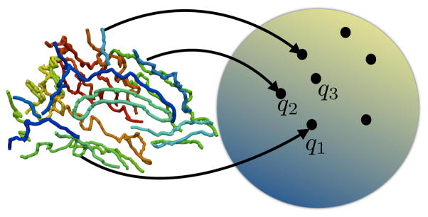
Schematic of the representation of the sulci on the shape space

To measure infinitesimal lengths and subsequently find geodesics in the shape space, we need a notion of a metric on the pre-shape space. We would like this metric to smoothly vary from one point to another and to have a convenient computational form. We therefore define a metric on the tangent space of shapes, and thereby induce it on the pre-shape space. Given a curve q ∈ , and the first order perturbations of q given by u, v ∈ T_q( ), respectively, the inner product between the tangent vectors u, v to at q is defined as,

$$\langle u,v\rangle ={\int }_0^{2\pi }{(u(s),v(s))}_{{ℝ}^3}ds.$$ (4)

It is observed that the metric given by Eq. 4 is a smooth, symmetric bilinear positive definite form, and is a Riemannian metric. Due to the spherical nature of the shape space, any vector on the shape space can be transformed to a tangent vector by simply subtracting its normal component. Thus the tangent space of is given by

$$T_q({\mathbb{S}}^q)=\{w\}\mid {\int }_0^{2\pi }{(w(s),q(s))}_{{ℝ}^3}ds=0,\forall s\in [0,2\pi ),$$ (5)

where w(s): I ≡ [0, 2π] → ℝ³. Here the set {w} represents all tangent vectors in the tangent space of .

Our goal is to seek an unique invariant representation by considering an equivalence class of all transformations such as rotations and reparameterizations that leave the shape of the curve unchanged. This issue is addressed in the next section by defining a quotient space of shapes, where geodesics, and thus the matching between curves is achieved by constructing the space of elastic shapes, and measuring the “elastic” distance between curves under certain well-defined shape-preserving transformations.

C. Geodesic Sulcal Matching on the Shape Space

Since we assume a continuous curve representation for sulci, in addition to translation and scaling, we consider the following transformations of the curve that preserve the sulcal shape. A rigid rotation of a curve is a shape-preserving operation, also considered as a group action by a 3×3 rotation matrix O₃ ∈ SO(3) on applied at q, and is defined as O₃·q(s) = O₃q(s), ∀s ∈ [0, 2π]. Lastly but importantly, curves can assume arbitrary speeds without changing the shape giving rise to multiple parameterizations that represent the same sulcal shape. This ambiguity in representation can be denoted by a new group action constituting a reparameterization by a non-linear map γ that changes the speed of the sulcus. In order to ensure that the ordering of the points on the sulci remain the same after reparameterization and that the speed function does not exhibit sharp jumps and discontinuities, a desirable property of this function γ is that it remains differentiable and also has a differentiable inverse. The class of functions that exhibit this property are also referred to as diffeomorphisms. We define = { γ: → } as the space of all orientation-preserving diffeomorphisms. Then the resulting variable speed parameterizations of the curve can be thought of as diffeomorphic group actions of γ ∈ on the curve q, and is derived as follows. Let q be the shape representation of a curve β. Let α = β(γ) be a reparameterization of β by γ. Then the velocity vector can be written as α̇ = γ̇β̇(γ). From Eqn. 1, we have $\stackrel{.}{\alpha }=\stackrel{.}{\gamma }\stackrel{.}{\beta }(\gamma )=\stackrel{.}{\gamma }q(\gamma )\Vert q(\gamma )\Vert =\Vert \sqrt{\stackrel{.}{\gamma }}q(\gamma )\Vert \sqrt{\stackrel{.}{\gamma }}q(\gamma )$. Reconstituting the velocity vector in terms of the shape function q, the reparameterization of q by γ is denoted as a right action of the group on the set as ϕ_γ(q), where ϕ: × → and is written as

$${\varphi }_{\gamma }(q)=q·\gamma =\sqrt{\stackrel{.}{\gamma }}(q\circ \gamma ).$$ (6)

Ultimately, we are interested in analyzing the sulci in the invariant space of shapes given by the quotient space of , modulo shape preserving transformations such as rigid rotations and reparameterizations. Consequently, the provision of the reparameterization operation facilitates elastic shape analysis of sulcal curves. We thus define the elastic shape space as the quotient space = /(SO(3) × ). Given a pair of shapes, the corresponding distance is then calculated as the length of the shortest path or a geodesic between the respective equivalence classes on the shape space . Before describing the method for computing geodesics in the space , it is simpler to understand this procedure for the pre-shape space .

1) Sulcal Geodesics in the Pre-shape Space

Given a pair of sulcal curves β₁, β₂, we first obtain their shape representations q₁, q₂ using Eqn. 1 by projecting them to the shape space. For the two shapes q₁ and q₂, the translation and scale invariant shape distance between them is found by measuring the length of the geodesic connecting q₁ and q₂ on the sphere . We know that geodesics on a sphere are great circles and can be specified analytically. Thus given a tangent vector f ∈ T_q1( ) in the direction of q₂, the geodesic on between the two points q₁, q₂ ∈ along f, for an infinitesimal time t is given by

$${\chi }_t(q_1;f)=cos(t{cos}^{-1}\langle q_1,q_2\rangle )q_1+sin(t{cos}^{-1}\langle q_1,q_2\rangle )f.$$ (7)

On a sphere, this tangent vector f can be computed as follows. First we find the angle between the two vector valued functions q₁, and q₂ as θ = arccos{< q_1,q₂ >}. The initial direction is given by f = q₂− < q₁, q₂ > q₁. The vector f is then projected in the tangent space at q₁, as $f=\frac{\theta ·f}{\sqrt{<f,f>}}$. We take incremental steps in the direction of f for short time intervals dt, to obtain successive shapes along the geodesic while projecting the tangent vector f on the tangent space at the consecutive shape. Then the geodesic distance between the two shapes q₁ and q₂ is given by

$$d(q_1,q_2)={\int }_0^1\sqrt{\langle {\stackrel{.}{\chi }}_t,{\stackrel{.}{\chi }}_t\rangle }dt$$ (8)

The quantity χ̇_t is also referred to as the tangent vector along the geodesic path χ_t. It is also noted that χ₀(q₁) = q₁, and χ₁(q₁) = q₂. By constructing geodesics on the pre-shape sphere ( ), we implicitly assumed that the curves were rotationally aligned and that the parameterizations of the curves were fixed at the onset of matching. This limitation is addressed in the next section where we find geodesics fully invariant to pose, scale, rotation as well as reparameterizations of sulci. Figure 3 shows a schematic and an example of a geodesic between two sulci on the sphere .

Figure 3.

Example of a geodesic between a pair of sulci (the first and the last shape along the geodesic) on .

2) Sulcal Geodesics in the Shape Space

In this section, we describe the procedure for finding an elastic reparameterization-invariant geodesic between shapes q₁ and q₂ that yields a diffeomorphic mapping between pairs of sulci. To motivate the discussion, we observe the comparisons between geodesics with and without scale and rotation invariance respectively in Fig. 4. From visually observing the deformations, it is clear that the sulcal matching is indeed affected by both scale and rotation. In our work, we achieve fully invariant matching between sulci by removing the effects of global rotation and scaling from the representation.

Figure 4.

Examples of geodesics with and without rotational (top) and scale (bottom) invariance between the first and the last curves respectively. The last curve was rotated and scaled according to the values displayed in the legend. The curves in the top row and the bottom row are color coded according to the rotation and the scale incurred by the target curve respectively. The geodesics for different rotations and scales are overlaid on top of each other.

Since the actions of the re-parametrization groups SO(3) and on constitute actions by isometries, we will find a geodesic between the equivalence classes of q₁ and q₂ by fixing the parameterization of q₁ and iteratively reparameterizing and re-orienting q₂ according to (O₃q₂) · γ, where O₃ ∈ SO(3), γ ∈ , such that the length of the geodesic path given by

$$d_e(q_1,q_2)=\underset{O_3\in SO(3),\gamma \in \mathcal{D}}{min}d(q_1,(O_3{q}_2)·\gamma )$$ (9)

is minimized. Here d is the geodesic distance given by Eqn. 8. This procedure is described below.

(a) Optimization over the rotation group SO(3)

The optimal rotation Ô₃ at each step is is found numerically by performing singular value decomposition of $q_1{q}_2^T$. We approximate the decomposition by the function as

$${\mathit{USV}}^T={\int }_0^{2\pi }{q}_1(s)q_2{(s)}^{T}ds,$$ (10)

where U, S, V ∈ ℝ^3×3. This yields the optimal rotation Ô₃ = UV^T.

(b) Optimization over the diffeomorphic group

The goal here is to find the optimal diffeomorphism γ̂ such that Eqn. 9 is minimized. We start by defining an orbit of the shape q₂ under the group action by a given γ ∈ . The optimality condition implies that the tangent vector χ̇₁ ∈ T_q2( ) is orthogonal to . In order to construct the tangent space T_q2 ( ), we first define a 1-parameter flow at the tangent space of at identity ψ_t: T_id( ) → , where T_id( ) = ( ), and id = s. We further note that given a tangent vector g ∈ T_id( ), we have ψ₀(id, g) = s, where s is the standard arc-length parameterization. The push-forward map of the group action in Eqn. 6 is given as

$${\varphi }_{\gamma \ast }(g)=\stackrel{.}{q}(s)g(s)+\frac{1}{2}q(s)\stackrel{.}{g}(s),s\in [0,2\pi )$$ (11)

We denote a Fourier basis for T_id( ) by V ≡ {v_i}, i = 1 … d, and define the projection of the tangent vector χ̇₁ on as

$$\pi ({\stackrel{.}{\chi }}_1)=\sum _{i=1}^d\langle {\stackrel{.}{\chi }}_1,{\varphi }_{\gamma \ast }(v_i)\rangle {\varphi }_{\gamma \ast }(v_i)$$ (12)

Then the optimality condition can be re-written as

$${\widehat{\stackrel{.}{\chi }}}_1=\underset{{\stackrel{.}{\chi }}_1}{argmin}\langle \pi ({\stackrel{.}{\chi }}_1),\pi ({\stackrel{.}{\chi }}_1)\rangle$$ (13)

Eqn. 13 is expanded in terms of the Fourier basis and minimized using gradient descent on the Fourier coefficients of V in the tangent space of T_id( ). At each iteration of the gradient procedure, we use the pull-back form of Eqn. 12 to construct g ∈ T_id( ) as

$$g=\sum _{i=1}^d\langle \langle {\stackrel{.}{\chi }}_1,{\varphi }_{\gamma \ast }(V)\rangle ,v_i\rangle v_i$$ (14)

to obtain the current estimate of the diffeomorphism γ = ψ₁(id, g). This diffeomorphism is used to obtain the new reparameterization q₂ · γ, and consequently the new estimate of χ̇₁. This procedure is repeated until Eqn. 13 converges.

(c) Reparameterization invariant and inverse-consistent mapping

The Riemannian metric proposed in Eq. 4 is invariant to reparameterizations. This can be easily verified as follows. Let {f_1,f₂} be a pair of tangent vectors at a shape q in the tangent space . Let γ: [0, 2π] → [0, 2π] be a reparameterization function acting on q as γ · q. Then the pair of reparameterized tangent vectors at γ · q is given by { $\sqrt{\stackrel{.}{\gamma }}{f}_1(\gamma (s)),\sqrt{\stackrel{.}{\gamma }}{f}_2(\gamma (s))$}. The inner product between the new pair of tangent vectors is given by ${\int }_0^{2\pi }{(\sqrt{\stackrel{.}{\gamma }}{f}_1(\gamma (s)),\sqrt{\stackrel{.}{\gamma }}{f}_2(\gamma (s)))}_{{ℝ}^3}ds$. Substituting t = γ(s) in the inner product, and noting that dt = γ̇(s)ds, we have ${\int }_0^{2\pi }{(f_1(\gamma (s)),f_2(\gamma (s)))}_{{ℝ}^3}\stackrel{.}{\gamma }(s)ds={\int }_0^{2\pi }{(f_1(t),f_2(t))}_{{ℝ}^3}dt$. This implies that when finding the optimal geodesic path between two shapes q₁ and q₂ we can keep one shape (say q₁) fixed, and reparameterize q₂ without changing the metric. We initialize the optimization procedure given in Sec. II-C2 by using dynamic programming [45] as the first step. Given the original shapes q₁ and q₂ we fix the initial rotation by performing a SVD according to Eqn. 10 and obtain an initial rotation O_init, and consequently the rotated shape $\stackrel{\sim }{q_2}=O_{\mathit{init}}{q}_2$. We then solve for the initial reparameterization by solving the following equation,

$${\gamma }_{\mathit{init}}=\underset{\gamma }{argmin}\left({\int }_0^{2\pi }[{\Vert q_1-\gamma ·\stackrel{\sim }{q_2}\Vert }^2+{\Vert \stackrel{\sim }{q_2}-{\gamma }^{-1}·q_1\Vert }^2]ds\right).$$ (15)

Since γ is a differentiable and invertible function, from the inverse function theorem, Eq. 15 can be written as

$${\gamma }_{\mathit{init}}=\underset{\gamma }{argmin}{\int }_0^{2\pi }\left[{\Vert q_1-\sqrt{\stackrel{.}{\gamma }}\stackrel{\sim }{q_2}(\gamma (s))\Vert }^2\right]ds+{\int }_0^{2\pi }\frac{1}{\stackrel{.}{\gamma }{\gamma }^{-1}}\left[{\Vert \sqrt{\stackrel{.}{\gamma }{\gamma }^{-1}}\stackrel{\sim }{q_2}-q_1({\gamma }^{-1}(s))\Vert }^2\right]ds$$ (16)

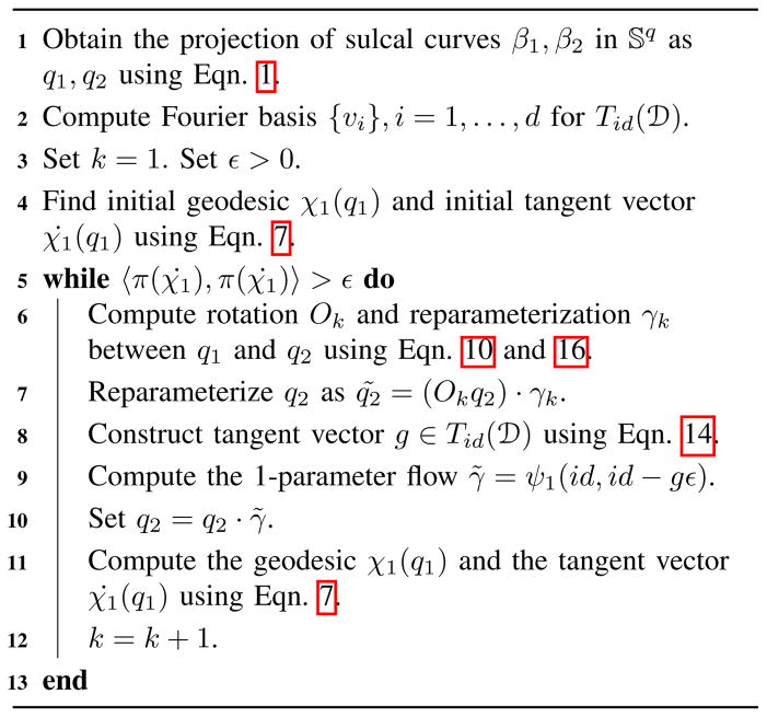
The above optimization techniques to compute sulcal geodesics in the shape space are presented in a step-wise manner in Algorithm 1.

Algorithm 1.

Geodesics between sulcal curves β₁ and β₂ in = /(SO(3) × )

Figure 5 shows comparisons of sulcal geodesics in the pre-shape space as well as in the invariant shape space. The pre-shape space geodesics, also known as extrinsic geodesics are obtained using Eqn. 9 by setting γ = s. It can be observed that unlike the extrinsic geodesics, the diffeomorphic geodesic deformations preserve sulcal shape homologies by automatically aligning critical features present in both sulci. Analogously in the extrinsic case, there is a loss of geometric alignment that results in a mismatch of sulcal features. Furthermore, regions of sulci where there is no obvious perceived alignment or matching show gradual transformation along the geodesics. Additionally, in order to demonstrate inverse-consistency of the sulcal mapping, Fig. 6 shows forward and backward (reversing the source and target shapes) geodesics between different pairs of sulci, along with the optimal repa-rameterizations obtained between the given pairs of shapes. For each column, the first path denotes a forward geodesic, and the second path denotes a backward geodesic. The two paths should be visually compared by following the first one from top to bottom, and the second one from bottom to top as shown by the arrows in the first column, and by noticing that the middle shapes along both the geodesics are most similar to each other. It is observed that the geodesics yield inverse consistent matching between shapes. This is further confirmed by overlaying the optimal parameterization γ₁ for the forward geodesic, along with the inverse optimal parameterization ${\gamma }_2^{-1}$ for the backward geodesic, and observing that they closely agree with each other.

Figure 5.

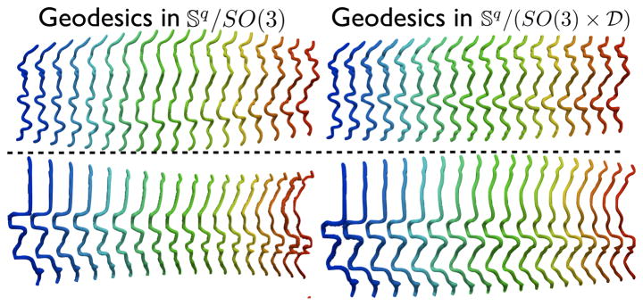
Left column: extrinsic geodesics in the pre-shape space invariant to translation, rotation and scaling. Right column: intrinsic geodesics in the shape space invariant to translation, rotation, scaling, and reparameterizations.

Figure 6.

Inverse consistency between the sulcal shape mappings. Each column shows a forward and backward geodesics between pairs of sulci (top row) as shown by the arrows in the first column. The optimal parameterization (γ₁) for the forward geodesic, as well as the inverse optimal parameterization ( ${\gamma }_2^{-1}$) for the backward geodesic are overlaid on top of each other (bottom row).

D. Construction of a Statistical Sulcal Atlas

For a collection of sulcal landmark curves, we now construct a statistical shape average for the entire set. Our objective here is twofold: create an atlas for a group/population analysis of the sulcal patterns, and utilize the diffeomorphic atlas for driving cortical registrations for a group of subjects. A related approach by Fletcher et al. [46] represents the population variability of object shapes on a manifold by geodesics between medial axis representations of shapes. In this work, we will also utilize non-linear geodesics between sulci, albeit on the shape space of curves. Based upon the homologous matching between individual sulci, it is desirable that the population average captures important statistical variabilities in the landmark data. While matching sulcal landmarks, we assume that the end points for all of the sulci of a particular type are identified. There are two well known approaches of computing statistical averages in nonlinear spaces. The extrinsic shape average is computed as an euclidean average of the shapes in the ambient space, and then subsequently projected back to the shape space. Despite its speed and computational simplicity, the extrinsic mean has a few limitations. It is ignorant of the specific nature of the representation of shapes, and thereby the underlying nonlinearity of the shape space. Furthermore it is sensitive to the method used for embedding the manifold in the euclidean space. As a simple example, a unit circle can be embedded inside ℝ² in several ways, and each embedding possibly leads to different values of extrinsic means on the circle. Importantly in the case of shapes, the extrinsic approach does not consider the elastic metric on the shape space and thus may not respect local shape homologies. Alternately, the intrinsic average is computed directly on the shape space, and makes use of distances and lengths that are defined strictly on the shape space. A major advantage of our sulcal representation and mapping framework is that it provides us with the necessary geometric structure to compute intrinsic statistical measures on the shape space. However, owing to the nonlinear, infinite-dimensional, and spherical nature of the shape space, the computation of the average shape is not straightforward, since we would like to compute the intrinsic mean shape in the quotient space of shapes . We use the well known definition of the Karcher mean [47], [48] to denote this intrinsic average and define it as follows.

Definition 1

Karcher Mean: For a set of shapes {q_i}, i = 1, …, N, the Karcher mean is given by

$$\mu =\underset{q_{\mu }}{argmin}\sum _{i=1}^N{d}_e{(q_{\mu },q_i)}^2,i=1,\dots ,N$$ (17)

The Karcher mean relies on the geodesics defined via the exponential map, and minimizes the average geodesic variance of the collection of shapes. The geodesic variance for N shapes is given by

$${\sigma }_g^2=\frac{1}{N}\sum _{i=1}^N\langle {{\stackrel{.}{\chi }}_1}^i(\mu ),{{\stackrel{.}{\chi }}_1}^i(\mu )\rangle ,$$ (18)

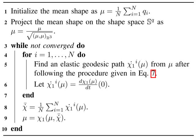
where the quantity χ̇₁ⁱ(μ) is calculated using Eqn. 13. Unlike the extrinsic mean, the Karcher mean is calculated by an iterative optimization procedure that involves repeated computations of geodesics from each of the shapes of the population to the current estimate of the mean. Algorithm 2 describes the procedure for computing the Karcher mean of a collection of shapes. As an illustration, Fig. 7 shows a schematic of the calculation of the extrinsic and the Karcher mean for a set of shapes. In this work, we will use the intrinsic approach by computing the Karcher mean for a given set of shapes.

Figure 7.

Schematic of the extrinsic and the intrinsic Karcher mean computation for a collection of shapes in .

Algorithm 2.

Computation of Karcher mean shape for a collection of shapes {q_i}, i = 1, …, N

E. Sulcal Shape Homologies

The curves representing the fundi of the sulci and the ridges of the gyri partially encode the complexity of the cortex. For landmark based cortical analysis, it is desirable that the geometrical features associated with this complexity be preserved for both the pairwise sulcal registrations as well as group-wise registrations to an atlas. This is possible if both the geometrical representation as well as the shape analysis method respect the observed biological sulcal shape homologies present in any given population. Conventional linear matching of sulcal curves assigns equal weights to all infinitesimal segments of the curve and simply computes a one-to-one mapping between two curves regardless of their intrinsic geometry. This is based upon a homeomorphism that is based upon equally weighted fractional distances from the starting point of the curve. This can result in a suboptimal matching of features on curves, and can lead to bumps on one curve corresponding to valleys on the other (See Fig. 5). As a consequence, when several of these sulci are pooled together from a population, these features can get weaker when averages are constructed. In contrast to this approach, our method shows a dramatic improvement in matching these features across sulci. Specifically, we suggest that the underlying geometric metric as well as the geodesics constructed using the metric are sensitive to the geometry of the sulci. While this is difficult to prove theoretically, we obtain experimental confirmation that the pairwise sulcal shape mappings demonstrate that salient geometrical features are matched from one sulcus to another. Moreover, the sulcal shape atlas constructed by finding repeated geodesics from all the sulci in the population to the mean shape also shows the presence of prominent global features that are characteristic of the population. This is depicted in Fig. 8, which compares the conventional euclidean sulcal matching with our approach. The left panel in Fig. 8 also shows the point-wise correspondences between sulcal pairs for both the diffeomorphic sulcal matching as well as the conventional euclidean sulcal matching approach. It is observed that the diffeomorphic matching enables better alignment of the ridges and valleys along the landmarks as compared to the euclidean matching. The right panel in Fig. 8 shows a comparison between the Karcher mean and the extrinsic euclidean mean for a set of 20 sulcal shapes. Furthermore, as expected, the euclidean average appears to have smoothed out detailed features pertaining to the ridges, and folds in the sample set compared to the Karcher mean. This idea is further investigated and experimentally verified for a large population of sulci in Sec. IV-A.

Figure 8.

Comparison between the extrinsic euclidean mean with the Karcher mean. Left panel shows point-wise correspondences between sample sulcal pairs for both non-elastic and elastic matching. Right panel shows the extrinsic euclidean mean and the Karcher mean for a sample of 20 sulcal shapes.

In the next section, we describe a procedure for combining the diffeomorphic sulcal shape atlas with a cortical registration framework that exploits the sulcal shape patterns for mapping brains across populations.

III. Cortical Surface Registration using Sulcal Homologies

In this section, we describe the method for cortical registration applied to models of the cortical pial surface that uses the presented sulcal matching framework. This registration process has three stages: (i) perform the matching of delineated sulcal landmarks, (ii) for each subject, parameterize the cortical surface to a unit square and (iii) find a vector field with respect to this parameterization that aligns the matched sulcal landmarks between subjects. The actual cortical registration uses a linear elastic energy for regularizing the displacement field. All the surfaces used in our analysis are assumed to have a spherical topology that is presumed to be enforced by the surface extraction method. In our studies, we used MNI tools [40] and Freesurfer [22] tools that do guarantee this constraint.

We define a set of N surfaces, {M₁, …, M_N} where M_i ⊂ ℝ³. We represent these surfaces discretely by manifold triangle meshes with spherical topology. For each surface i, we have a set of L landmarks represented by continuous open curves {β_i1, …, β_iL} where β_ij: [0, 2π] ↦ M_i, and the ordered set of points {β_ij: i ∈ [1, N], j ∈ [1, L]} represents homologous vertices on the set of surfaces. The curves are discretized as simple polylines, where the j-th curve has k_j vertices.

A. Inverse Diffeomorphic Mapping of Sulci

The first step of the process is to establish a correspondence between the homologous landmark curves by computing diffeomorphic mappings γ̂_ij: [0, 2π] ↦ [0, 2π] given by Algorithm 1 between shapes of sulci. We then apply the resulting diffeomorphisms γ̂_ij to the native sulci β_ij such that for curve j and parameter t, {β_ij(γ̂_ij(t)): i ∈ [1, N]} is a set of homologous points on the surfaces. This is accomplished by mapping the curves to a Riemannian manifold, where reparameterizations are defined by geodesics to the Karcher mean of the curves in the shape space. To avoid aliasing artifacts, each curve in a set is resampled with the maximal number of vertices in the set.

B. Spherical Mapping and Alignment

Next, the surfaces are mapped to the sphere to establish a parameterization in which the registration will be performed. The spherical mapping is initialized by subtracting the mean and normalizing all of the vertices, so that they are consistent with the pose and orientation of the input meshes. A set of bijective mappings is found from each surface to the unit sphere, {ϕ₁, …, ϕ_N} where ϕ_i: M_i ↦ S². The spherical mapping of the matched curves is then $\stackrel{\sim }{{\beta }_{ij}}={\varphi }_i\circ {\beta }_{ij}\circ {\widehat{\gamma }}_{ij}$. The meshes are simplified using QEM simplification [49] and mapped to a sphere using an unconstrained energy-based method [50]. The curves are then mapped to the sphere by finding the barycentric coordinates of each curve vertex in the nearest triangle. A bounded interval hierarchy is used to efficiently search for the coincident face of each curve vertex. Once the meshes and curves are mapped to the sphere, they are rotationally aligned to enforce a consistent orientation of the spherical mappings. Given an arbitrarily chosen target, each set of curves is aligned to the target by computing the rotation and reflection that minimizes the least-squared difference between the discretized curve coordinates. This is accomplished by solving the unconstrained orthogonal Procrustes problem using singular value decomposition. Typically, left and right hemisphere surfaces will be included and allowing reflections in the transform allows both hemispheres to be mapped to a common orientation. More formally, for an arbitrary $T\in \{\stackrel{\sim }{{\beta }_{ij}}:i\in [1,N]\}$, we find an alignment R ∈ ℝ^3×3

$$R_i=arg\underset{\mathrm{\Omega }}{min}\sum _j\sum _k\Vert \mathrm{\Omega }\left(\stackrel{\sim }{{\beta }_{ij}}\left(\frac{k-1}{k_j-1}\right)\right)-T\left(\frac{k-1}{k_j-1}\right)\Vert ,$$ (19)

where Ω^T Ω = I

The rotation is then applied to the sphere-mapped curves and meshes as, $\widehat{{\varphi }_i}=R_i\circ {\varphi }_i$, and $\widehat{{\beta }_{ij}}=R_i\circ \stackrel{\sim }{{\beta }_{ij}}$.

C. Spherical Curve Atlas

Once the meshes and curves have been aligned on the sphere, the mean curves are computed. These mean curves will be used as the atlas curves in the surface warping. The Karcher mean on the sphere is found for each vertex of each curve, across the group. In this method, an initial guess is found by the normalized average of the points. For this point, the tangent space is defined by the gnomonic projection. A new mean is computed in the tangent space, and it is mapped back to the sphere and the process is repeated until the difference between the previous and the new mean is smaller than a threshold. We can express the curve atlas as the set { $\overline{{\beta }_j}:j\in [1,L]$}, where $\overline{{\beta }_j}$ is the Karcher mean of { $\stackrel{\sim }{{\beta }_{ij}}:i\in [1,N]$}.

D. Elastic Surface Warping

For surface i, the deformation of the atlas is denoted by ϕ_i: S² ↦ S², where ${\varphi }_i(\overline{{\beta }_j}(t))=\widehat{{\beta }_{ij}}(t)$ for t ∈ [0, 2π], j ∈ [1, L]. Six bijective flattenings of the sphere, each topologically equivalent to cutting along the four edges that meet at one of the six vertices of an octahedron, are defined as {φ_n: S² ↦ [0, 1]^2: n ∈ 1, 2, 3, 4, 5, 6}. For a point on the sphere, p ∈ S², the flattening is chosen as ${\phi }_p=arg{min}_{{\phi }_n}\Vert {\phi }_n(p)-\left(\frac{1}{2},\frac{1}{2}\right)\Vert$. The displacement field u_p: S₂ ↦ ℝ² is then u_p(x) = φ_p(ϕ_i(x)) − φ_p(x). At non-landmark points, i.e. x ∈ S², $x\notin {\cup }_j\{\widehat{{\beta }_{ij}}(t):t\in [0,2\pi ]\}$, the mapping is constrained to satisfy a small deformation linear elastic model similar to Thompson et al. [28], and is given by

$$\mu {\nabla }^2{u}_p(x)+(\lambda +\mu )\nabla (\nabla ·u_p(x))=0$$ (20)

The atlas mesh is defined on the sphere by tessellating the sphere with a subdivided octahedron [51]. This tessellation provides convenient flattened representations and has computationally advantageous multiscale properties. Subdivision of each triangle is performed by adding vertices at the midpoints of the edges, adding new edges connecting them, and creating four triangles from the original. This scheme is used for defining the representations of the mesh in multiscale algorithms. Furthermore, this subdivision process ensures that the mesh can be flattened to a square and eventually a regularly sampled grid. One benefit of the planar mapping is that it greatly simplifies the implementation of finite difference and multigrid numerical methods and can also be implemented efficiently by a lookup table. This flattening can be imagined as follows. First, one of the vertices of the octahedron is chosen, and mapped to the center of the grid. Then four far edges that do not contain the center vertex are cut, and duplicated to define the boundary of the grid. Finally the vertex opposite to the one selected maps to the four corners of the grid. The flattening points (those that are mapped to the center of the grid for each of their respective mappings) lie on antipodal points at each of the three coordinate axes, which coincide with the vertices of the octahedron. These points were chosen to maximize the distance between points and to permit efficient flattening and numerical optimization. This flattened representation allows for efficient interpolation, smoothing and finite differences operations on the grid [51]. The spherical mapping, octahedral warping, and flattening is illustrated in Fig. 9.

Figure 9.

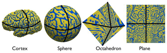
Mappings between the cortical surface, sphere, an octahedron, and a plane.

The deformation is computed iteratively using finite differences with a multigrid method, where prolongation, restriction and smoothing operations are performed on the flattened representation. The solver accounts for the spherical topology of the domain by solving the equation in the optimal flattening of the mesh at the vertex. The parameterization of each mesh is resampled by the deformation from the atlas, establishing vertex homology between the meshes. The cortical surface warping workflow is schematically illustrated in Fig. 10.

Figure 10.

Pipeline for cortical surface registration using the diffeomorphic sulcal shape homology. (See Sec. V for implementation).

IV. Results and Discussion

In this section we present results showing the diffeomorphic sulcal shape atlas based on two different populations. Additionally, we show results for cortical surface matching obtained using the sulcal shape atlas. The cortical data was derived from two different surface extraction methods that extract both shallow and deep sulci on the cortex. The same sulcal tracing protocol [9] was used to delineate curves on the cortex.

A. Diffeomorphic Sulcal Shape Atlas

This section presents experimental results showing the construction of a sulcal shape atlas obtained using Algorithm 2. The population data consisted of 176 subjects (age: 31.8 ± 9 years, sex: 105 males, 71 females, ethnicity: consistent with the demographics of the Los Angeles area) obtained after approval by the UCLA Institutional Review Board (IRB). These subjects underwent high-resolution T1-weighted structural MRI scanning on a Siemens 1.5 Tesla Sonata system using a 3D MPRAGE sequence (TR/TE = 1900 ms/28 ms; voxel size = 1 mm× 1 mm × 1 mm; TI = 1100; matrix size = 256 × 256 × 160; flip angle: 15°). After preprocessing the raw data and registering it stereotaxically to a standard atlas space, the cortical surfaces for these subjects were extracted using an automated algorithm [40], and sulci were traced according to the protocol illustrated in Fig. 1 [9]. Figure 11 shows the original unregistered 28 sulcal landmarks for the complete population of 176 subjects for the left hemisphere. Along with the sulcal population, Fig. 11 also shows the intrinsic, Karcher sulcal shape averages using Algorithm 2 for all of the 28 landmark curves, as well as the extrinsic shape averages for the same. The extrinsic averages are computed on the pre-shape space by using the same Algorithm 2, but setting γ = s at each step. Since the euclidean matching of sulci forces a one-one correspondence between them, under the uniform sampling assumption, the only remaining shape-preserving transformation after scale, and translation is removed is pairwise rotational alignment. The extrinsic euclidean average for all the sulci was thus computed on the shape space by factoring out rigid motions and scale. This is in contrast with the Karcher sulcal average which is computed after an additional invariance to reparameterization. For visualization purposes, both the Karcher averages, as well as the euclidean sulcal averages were instantiated in the curve space under an average translation, scaling and rotation all measured in their respective spaces, ℝ³, ℝ_{+}, and SO(3). It should be noted that the intrinsic averages although smooth, have preserved important features along the landmarks, thus representing the average local shape geometry along the sulci. This implies that the shape average has not only captured the salient geometric features, but has also reduced the shape variability in the population. In order to demonstrate this property, we plot the variance of the shape deformation for each landmark type as captured by the velocity vector along the geodesic path, both for euclidean extrinsic, and Riemannian intrinsic averages. Thus for each of the 28 landmark average shapes for 176 subjects, μ̂_i, i = 1, …, 28, we plot the geodesic variance ${\sigma }_g^2$ from Eqn. 18. The geodesic variance measures the invariant deformation between a pair of shapes, and only depends upon the intrinsic geometry of the shapes. Figure 11 shows a comparison of the plots of ${\sigma }_g^2$ for each of the landmarks, taken along the length of the curve, for both euclidean shape averages, as well as intrinsic shape averages. This can also be thought of as the geodesic variance. From the color-coded map, it is observed that the intrinsic average has reduced the variance in terms of shape geometry deformation, and thus is a better representative of the population. For further quantification of this result, we compared the geodesic variance averaged for each sulcus for both the euclidean and the diffeomorphic methods, displayed in Fig. 12. The variance displayed by the diffeomorphic method was significantly lower (when corrected for multiple comparisons at a threshold of p_FDR = 0.001) for all the sulci except the Central Sulcus. Fig. 12 shows a * symbol next to each sulcal label that showed a significant difference (p < 1e−3) in the variance between the two methods.

Figure 11.

Lateral, medial, and axial views of, First column: All 28 landmark sulci for 176 subjects, Middle column: euclidean sulcal shape averages for each landmark, Last column: Karcher means for each landmark. (Best viewed in color). In the middle and last column, sulci are color-coded according to the geodesic variance for the entire sulcal population for each of the 28 landmarks, both for euclidean shape averages, as well as elastic shape averages, along the length of the curves.

Figure 12.

Comparison of the geodesic variance averaged over each sulcus for the sulcal population for each of the 28 landmarks, for euclidean as well as diffeomorphic sulcal mapping averages, for the left hemisphere. The * denotes the sulci where the difference between the variance is significant.

Based on the discussion in Sec. II-E, the euclidean sulcal atlas shows weakened representation of bumps and wiggles along the curve. However an important question here is whether all the features manifested in the diffeomorphic population sulcal atlas really arise inherently from the data, and not as a result of noise or errors introduced in the matching process over the course of optimization? In order to experimentally verify that this is indeed not the case, we performed 100 randomized trials of sampling 8 disjoint subsets of 22 subjects each and computed the extrinsic and diffeomorphic averages for all the sulci in those subsets for each trial. We then computed the local curvature at each point on the average curves for each sulcus. Figure 13 shows the local curvatures overlaid on the extrinsic and diffeomorphic averages for the 100 trials. Comparing Figures 11 and 13, it is observed that even after sub dividing the population to a reduced number of subjects, the diffeomorphic method is able to detect conspicuous patterns present in the sulcal geometry. Furthermore almost all of the important sulci (including the inferior and superior frontal, inferior and superior temporal, as well as pre- and post-central sulci) display higher curvature than their counterparts in the euclidean atlases. If one assumes that curvatures of the landmark curves do contain partial information about the complexity of the cortex, then the results suggest that the diffeomorphic sulcal shape atlas contains more information than the euclidean sulcal atlas.

Figure 13.

Comparison of the euclidean and diffeomorphic sulcal atlases for eight different disjoint sub-populations of the original 176 subjects. The sub-populations were obtained after 100 randomized trials of sampling subsets of 22 subjects for each group. For each method, the sulcal atlases are overlaid on top of each other and color-coded by curvature of the curve.

Additionally, we performed t-tests comparing the average raw curvatures for both the methods. After correcting for multiple comparisons, we observed that the curvatures for diffeomorphic averages were significantly higher than their extrinsic counterparts. Figure 14 shows a bar chart of the local curvatures averaged over each sulcus after 100 randomized trials. The * next to the sulcus label denotes that the sulcal curvature showed a significant difference (p < 1e − 5), after controlling for FDR (p_FDR = 0.00001). The box plots along the bar graphs display the variance in the curvature in the 100 trials.

Figure 14.

Comparison of the local curvatures averaged over each sulcus under both euclidean and diffeomorphic mapping. The * denotes that the two curvatures were significantly different after controlling for FDR.

B. Cortical Mapping for Surfaces extracted using the MNI [40] protocol

We now demonstrate results of cortical surface registration with and without the incorporation of the diffeomorphic matching for sulcal shape analysis. The data consisted of same set of cortical surfaces used in Sec. IV-A. The sulcal shape atlas is already constructed and shown in Fig. 11. We now compute geodesics between the average shape of the landmark and the set of all sulci belonging to that landmark type and reparameterize the set of sulci according to inverses of the resulting diffeomorphisms. We then follow the steps outlined in Sec. III in order to warp all the surfaces meshes to the atlas. Figure 15 shows the flattened representation of a surface atlas colored according to curvature of the surface using both euclidean analysis and diffeomorphic shape analysis. Additionally, Fig. 15 shows the lateral, dorsal, and medial views of the reconstructed cortical surface from the flattened representations. It is observed that the surfaces using intrinsic sulcal analysis exhibit rich local geometry that has been preserved due to the elastic diffeomorphisms.

Figure 15.

Top row: Average flattened representations for atlases: with landmark curves using euclidean matching (left), with landmark curves using the diffeomorphic matching (right). Remaining rows show lateral, ventral, and medial views of the reconstructed cortical surface with euclidean matching (left) and diffeomorphic matching (right). The flat maps and the surfaces are color coded according to curvedness.

Cortical Mapping for Surfaces extracted using the Freesurfer [22] protocol

Our experimental data consisted of 3T MRI acquisitions (GE) for a population of 69 subjects (age: 25.5 ± 10.6 years, sex: 30 males, 39 females, ethnicity: Chinese) acquired using the Shandong University IRB approved study. The scanning protocol involved a transverse 3D T1-weighted fast spoiled gradient-echo (FSPGR) sequence (TR/TE = 6.8 ms/2.9 ms; voxel size = 0.47 mm × 0.47 mm × 0.70 mm; matrix size = 512 × 512; flip angle = 10°, slice thickness = 1.4 mm, and slice gap = 0.7 mm). After preprocessing the raw data and registering it stereotaxically to a standard atlas space, the cortical surfaces for these subjects were extracted using an automated algorithm [21]. It is noted that these surfaces obtained using the Freesurfer protocol exhibit greater sulcal depth than those obtained using the MNI protocol in Sec. IV-B. The original sulcal tracing protocol was developed on the MNI surfaces and thus was subsequently adapted to deal with Freesurfer surfaces as well. Accordingly, we selected a total of 27 landmark curves on the Freesurfer surfaces for the purpose of constructing the Chinese atlas. Figure 17 shows the 27 sulcal landmarks for all of the 69 subjects for both hemispheres overlaid together. Using this set of sulcal curves, we proceed to follow the same steps in Sec. IV-B to compute the diffeomorphic as well as euclidean sulcal averages for the population. Figure 17 shows the diffeomorphic sulcal shape averages, as well as the respective extrinsic euclidean averages for this group. Again, all the averages were computed by mapping of the native curves to the shape space. The shape space averages were then projected back in the the native space of curves in order to obtain Fig. 17. Similar to the results in Sec. IV-B, it is observed that the intrinsic averages were smooth but preserved important features along the landmarks implying that the shape average have captured the salient geometric features and also have reduced the shape variability in the population. Similar to Sec. IV-B, we plot the variance of the shape deformation for each landmark type as captured by the velocity vector along the geodesic path for the euclidean extrinsic and the Riemannian intrinsic averages in Fig. 16 for both the hemispheres. From the variance bars, it is observed that the intrinsic average has reduced the variance in terms of shape geometry deformation compared to the extrinsic average and thus is a better representative of the population. This result is also consistent with the results in the previous section (Sec. IV-B). We also tested for statistical significance in the differences between variances and found that the geodesic variances obtained using the diffeomorphic method was highly significantly different from the extrinsic result, even when corrected for multiple comparisons using the false discovery rate (FDR). For the left hemisphere, all the sulci showed significantly lower variance (p < 1e − 6) when FDR thresholded at p_FDR = 0.0059, whereas in the right hemisphere, all the sulci except the Sylvian fissure showed a significantly lower variance (p < 1e − 6) when thresholded at p_FDR=0.0014. The significant sulci are represented by the * symbol in Fig. 16. Also see Sec. IV-C for the experimental results obtained using the Freesurfer sulcal alignment, also plotted in Fig. 16.

Figure 17.

Lateral left and right, and axial views of: 27 landmark sulci for each of the 69 subjects (first column), euclidean sulcal shape averages (second column), and Karcher shape average (third column) for each landmark type overlaid on the average surface. The sulcal shapes in the second and the third column are colored according to the geodesic variance of the population.

Figure 16.

Comparison of the geodesic variance averaged over each sulcus for the entire sulcal population for each of the 27 landmarks, for euclidean shape averages, Freesurfer-aligned sulcal averages, as well as diffeomorphic shape averages, for both the left (top row), and the right (bottom row) hemispheres. The * symbol denotes the sulci for which the variance is significantly different between the diffeomorphic method and the euclidean and the Freesurfer alignment.

Next, we demonstrate results of cortical surface registration with and without the incorporation of the above diffeomorphic sulcal atlas in Figure 17. As an initial step, we compute geodesics between the average shape of the landmark and the set of all sulci belonging to that landmark type and reparameterize the set of sulci according to inverses of the resulting diffeomorphisms. We then follow the steps outlined in Sec. III in order to warp all the surfaces meshes to the atlas. Figure 18 shows the lateral, axial, ventral, and medial views of the reconstructed cortical surface averages from the flattened representations. The surface is colored by its curvedness in order to highlight the fundi of the sulci as well as the ridges of the gyri. It is observed that the surface with diffeomorphic sulcal mapping shows richer geometric detail than the traditional euclidean reconstruction.

Figure 18.

Lateral, axial, ventral, and medial views of the reconstructed cortical surface with spherical alignment without landmarks (top), euclidean sulcal matching (middle), and diffeomorphic sulcal matching (bottom). Shape curvedness is calculated for each surface, thresholded according to the displayed color scale, and overlaid on all the surfaces.

We also computed the local Jacobian determinants of the mapping from each subject to the mean surface for both the extrinsic and the diffeomorphic methods following the procedure given in [52]. Assuming a smooth mapping Φ from each surface M_i to the mean given by Φ: M_i → M_μ, where M_μ is the surface atlas, the differential mapping d_Φ: T_v(M_i) → T_Φ(v)(M_μ), v ≡ [v₁, v₂, v₃]^T ∈ ℝ³, can be approximated up to a first order and discretely represented by the Jacobian J given by J = [Φ(v₃) − Φ(v₁), Φ(v₂) − Φ (v₁)][v₃ − v₁, v₂ − v₁]⁻¹. Similar to Wang et al. [52], we compute a deformation tensor $S=\sqrt{J^{T}J}$, and compute its determinant. In the discrete setting, we project the two corresponding triangle faces on a planar domain that represents a locally linear tangent space to the surface at a point denoting the midpoint of the face and then compute the two-dimensional displacement vectors to form the matrix J at each point on the surface. We then compared the Jacobian determinants for all point on the surface for all the subjects with respect to the mean for both euclidean and diffeomorphic mapping. All determinants for both the methods were strictly positive. Fig. 19 shows the p-map (after correcting for multiple comparisons at a FDR threshold of p_FDR = 0.0031) for a t-test between the Jacobian determinants for both cases. It is observed that there are significant differences in the warping between both methods in the vicinity of the sulci. It was also observed (not shown in the figure) that the determinants for the diffeomorphic case were larger in magnitude compared to the euclidean case. One possible interpretation of this result is that the diffeomorphic mapping incurs larger deformations when it attempts to bring the shape of the sulcus under alignment compared to the euclidean mapping. Since the sulcal geodesics are constructed on the shape space, the geodesic distances between sulci under the diffeomorphic mapping are greater than the geodesic distances in the ambient space, as is the case for the euclidean matching. Consequently there is a larger cost in deforming sulci diffeomorphically instead of extrinsically and this is reflected in the Jacobians of the warps under both methods.

Figure 19.

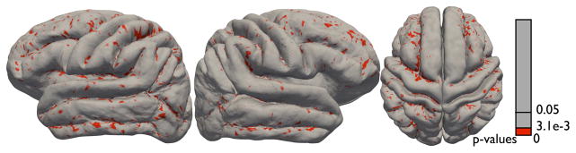
Comparison of the Jacobian determinants between the diffeomorphic and euclidean mapping. The colormap shows p-values (after correcting for the false discovery rate) overlaid on the diffeomorphic atlas surface.

C. Comparison to a Cortical Atlas without explicit sulcal constraints

In this section, we compare the cortical atlas obtained using diffeomorphic sulcal matching using Freesurfer [22], which implements a fully automated algorithm for cortical warping and atlas construction. Freesurfer utilizes diverse local and global criteria such as local cortical curvature along with sulcal depth and automatically aligns cortical surfaces for a population of subjects. For evaluation purposes, we compared the following three experimental results, a) automatic Freesurfer cortical registration, b) diffeomorphic sulcal shape-based cortical registration, and c) a combined approach of first using Freesurfer cortical registrations and then warping the resulting registered spherical cortices combined with the sulcal curves mapped using our diffeomorphic approach. The last experiment was performed as follows: i) The individual pial surfaces obtained from Freesurfer were resampled to the Freesurfer average template subject to have the same number of vertices and faces throughout the population. ii) For each subject, the sulci were then projected on to the resampled surface. iii) The spherical coordinates of the sphere-resampled pial surface were stored as per-vertex attributes in the pial surface itself and these augmented pial surfaces and curves were provided as an input to our diffeomorphic warping workflow. While executing the algorithm, we disabled the sphere mapping step, choosing to utilize the Freesurfer generated spherical coordinates instead. The output of the diffeomorphic workflow then resulted in the cortical registrations that respected both the additional constraints that Freesurfer imposed previously as well as the explicit sulcal shape constraints that we calculated. Figure 20 shows the average surfaces resulting from the three experiments. As a measure of distortion, we also computed the root mean square (r.m.s.) error of the distance from each sample surface to the average reconstructed cortical surface and overlaid it on the average (20) for each of the results. For the Freesurfer registration, it is observed that the Freesurfer displacement is higher in some regions such as the left and right frontal lobe, the left temporal lobe, and the left and right parietal lobe, compared to the diffeomorphic approach, whereas it is lower in regions such as the Sylvian fissure. At the same time, it is also observed that on the account of Freesurfer’s local and global constraints on curvature and depth, in the case of the occipital lobe, the Freesurfer average shows more details than the diffeomorphic approach, where there were only a few sulci guiding the registration. For the combined Freesurfer and diffeomorphic approach, it is observed that the r.m.s. displacement was reduced in the places where it was higher previously, and there is an emergence of details in the cortical patterns in the occipital lobe. Additionally, the displacement in the Sylvian fissure was reduced considerably, where the matching discounted explicit sulcal constraints. At the same time it should be noted that the Freesurfer matching criteria and energy functions are different from our approach, hence there is an interplay of these energies in the final results where both the Freesurfer and diffeomorphic registrations are combined. As a result, the solution may not always be jointly optimal with respect to both non-explicit depth, and curvature and explicit sulcal constraints.

Figure 20.

R.M.S. error of the distance from each sample surface to the average surface for automatic cortical warping for (first column) Freesurfer-based [22] warping, middle column (diffeomorphic warping), and (last column) combined intermediate Freesurfer spherical warping and diffeomorphic landmark mapping.

Lastly, aside from the cortical surfaces, we also investigated the sulcal alignment and mapping resulting from the automatic Freesurfer registration. We followed steps i) and ii) of the above experiment to obtain the projected sulcal curves from the resampled Freesurfer surfaces. These registered landmarks were then projected on the shape space, removing the translation and scale but keeping the non-uniform parameterization intact. These projected sulcal curves can be represented as the set { ${\beta }_{ij}\circ {\widehat{\gamma }}_{ij}^{FS}(t)$: i = 1 … 69, j = 1 … 27}, where {β_ij} is the set of native sulci and ${\widehat{\gamma }}_{ij}^{FS}$ is the automatic Freesurfer optimal resampling. We projected these resampled sulci on the pre-shape space and computed the extrinsic geodesic variance as described in Sec. II-E. It is noted that the optimal Freesurfer resampling is kept intact in this procedure, since we do not change the curve reparameterizations when computing the extrinsic geodesic variance. Thus the Freesurfer sulcal alignment can also be thought of as an optimal reparameterization of the sulcal curves under automatic curvature-based constraints. This makes the respective variances comparable, since they are computed on the same shape space and under the same metric (inner-product) using the same algorithm. Figure 16 displays the Freesurfer aligned sulcal geodesic variance in comparison with the extrinsic euclidean and the diffeomorphic geodesic variance. It is observed that variance due to the Freesurfer alignment is smaller than the extrinsic variance, but significantly (left hemisphere, p < 1e − 6, p_FDR = 0.0059) greater than the diffeomorphic case. In the case of the Sylvian fissure, Freesurfer had a lower geodesic variance than the diffeomorphic case, but the differences were not significant.

D. Sulcal Shape Classification

The shapes of the individual sulcal curves are influenced by the intrinsic cortical folding patterns. This shape variability has been exploited in the problem of sulcal labeling and classification in the context of detection and extraction of sulci [53], [36], [54], [7], [55], [56], [57]. In order to determine the discriminative characteristics of our geometric sulcal representation, we classify sulcal shapes by performing discriminative pattern analysis of the sulcal shapes. For the purpose of classification, we consider the dataset of 176 subjects described in Sec. IV-B and randomly divide it into a training set and a testing set of 88 subjects each. We then compute the mean shapes for each of the 28 sulcal types for the training set and denote them by { ${\mu }_k^{\mathit{train}}$}, k = 1, …, 28. We then compute geodesic distances from each sulcus for each subject to the training mean shapes and use a minimum distance classifier to label each of the sulci according to the 28 classes. Additionally we included pose information (location only) from the sulcal curve in the classifier. For a given sulcus $q_i^j$, j ∈ [1, 88], the labeled class, k̂ ∈ [1, 28] is given by

$$\widehat{k}={\text{argmin}}_k[w_1{d}_e{(q_i^j,{\mu }_k^{\mathit{train}})}^2+w_2{\Vert {\beta }_{q_i^j}(\pi )-{\beta }_{{\mu }_k^{\mathit{train}}}(\pi )\Vert }^2],$$ (21)

where i, k = 1, …, 28, j = 1, …, 88, and ${\beta }_{q_i^j}(\pi )$, and ${\beta }_{{\mu }_k^{\mathit{train}}}(\pi )$ are the center positions of the native space curve representations of $q_i^j$ , and ${\mu }_k^{\mathit{train}}$ , and w₁ and w₂ are the weights assigned (chosen experimentally) to the shape distance and the pose distance respectively. We performed 50 trials of the above experiment by randomly dividing the population into two groups and computed the average classification recall rate separately for each sulcus (proportion of the correctly labeled sulci from the random subset of 88 subjects) using the one-against-all rule. The complete labeling results for the randomized trials for three cases are described as follows: (a) Pose-only classification (w₁ = 0, w₂ = 0.01): Figure 21(A) shows the sulcus-wise percent recall rate based on differences in location alone. Almost all (23/28) sulci showed a greater than 92~94% recall rate, with the superior temporal sulcus showing a 100% recall rate for each trial. The sulci that underperformed significantly (< 80%) are the olfactory sulcus (74%), the inferior (76%) and the superior callosal boundary (80%), and the olfactory control line (77%). This is because the callosal boundaries and the olfactory sulci were misclassified since they are close together. (b) Shape-only classification (w₁ = 1, w₂ = 0): Figure 21(B) shows the recall rate based only on shape discrimination under the extrinsic as well as the diffeomorphic shape metric. We observed that 11/28 sulci showed a high recall rate (> 93%). Moreover it was remarkable that both the shape metrics were able to successfully differentiate between the inferior and the superior callosal boundaries 100% of the time. Furthermore, for specific sulci such as the intraparietal sulcus, olfactory control line, central sulcus, precentral sulcus, paracentral sulcus, inferior frontal sulcus, and the precentral marginal sulcus, the diffeomorphic method yielded significantly improved success rates (5~11%) over the extrinsic method. It is also observed that the recall rate for the olfactory sulcus has substantially improved due to shape matching. In the case of the trans occipital, and the calcarine ant. sulcus, the euclidean metric showed a better performance than the diffeomorphic metric. A possible explanation is that the lengths of these sulci are significantly smaller compared to all the other sulci, and for shape-only classification, we enforce an unit length constraint on these sulci. Our reasoning is that due to this constraint, the shape matching may have favored the euclidean metric vs the diffeomorphic metric. Additionally, the superior temporal sulcus showed a very mild improvement with the euclidean metric, but the result was not statistically significant. (c) Combined Shape and Pose classification (w₁ = 1, w₂ = 0.01): Finally Fig. 21(C) shows the recall rate for joint shape and pose classification for both the extrinsic and the diffeomorphic shape measures. This time, in the case of the diffeomorphic matching, all of the sulci show a recall rate greater than 90% with 22/28 sulci showing a recall rate greater than 98%. In the case of the olfactory sulcus the overall combined recall rate has decreased compared to the one based on shape alone, since the pose classification interferes with the shape classification.

Figure 21.

Percent recall rate for each sulcus based on A) Pose location only, B) Shape matching only, and C) combined shape and pose matching.

We achieved significantly higher recall rates using both the shape and location of the individual sulci together compared to using both of them individually. These rates can be considerably improved further by considering joint configurations of sulcal shapes, their relative locations, as well as scales and orientations with respect to each other.

V. Notes on Implementation

The sulcal protocols used in this paper can be downloaded from the LONI Sulcal Protocol http://www.loni.ucla.edu/~esowell/edevel/new_sulcvar.html, and the Damasio Curve Protocol [58] (http://neuroimage.usc.edu/CurveProtocol.html). The methods discussed in the paper are implemented in Java and are completely cross-platform. The binaries as well as source code files are freely available from LONI ShapeTools (http://www.loni.ucla.edu/twiki/bin/view/CCB/ShapeToolLibraryProgram). In addition to the individual modules, an integrated workflow is also available for download at LONI MAST Surface Warping Pipeline http://www.loni.ucla.edu/twiki/bin/view/MAST/ElasticSurfaceWarpProtocolDownload. This workflow can be executed from the LONI pipeline [59] interface both on a multi-node compute cluster, as well as a standalone workstation. After undergoing tracing training, sulci can be delineated swiftly using either ShapeTools ShapeViewer or Brainsuite on an average of 10~15 minutes per brain, with the tracing time improving rapidly with experience. In the same pass, we determine the maximum number of vertices across all the sulci and uniformly resample all the vertices of the sulci to this number. It is noted that this resampling preserves the shapes of the sulci and does not affect the pose, orientation, or even the scale of the curves. Since these sulci are manually delineated, we do not incur aliasing effects, except at the point of tracing. Furthermore, when tracing the curves, either using Shapeviewer or Brainsuite, the interface is designed in such a way that, even when the user clicks a limited set of points, the tracing program estimates a dense curve passing through all the vertices on the surface along the path of the clicked points. The execution time for the complete workflow for a set of 176 subjects on a stand-alone workstation (Intel Xeon, 8 core, 2.5 GHz) was approximately 10 hours, including both hemispheres. While the running time could be reduced further by reimplementing the methods in C++ and using standard optimization packages, our focus was on cross-platform portability and ease of distribution and use.

VI. Conclusion

We have presented a diffeomorphic approach for sulcal shape representation and mapping and have demonstrated its applicability to population based sulcal shape analysis, cortical surface registration, and sulcal shape classification. The method uses a novel square-root velocity representation for elastic curves and a Riemannian metric for matching shapes. The metric is invariant to rigid motions as well as speed-reparameterization, an important requirement for diffeomorphic matching. Experimental results seem to suggest that the shape matching methodology respects the underlying biological patterns manifested on the landmark curves through the cortex. The diffeomorphic sulcal shape atlas also exhibits higher curvature values throughout the curves compared to the euclidean sulcal atlas. This further confirms that the diffeomorphic method is indeed preserving feature-rich information in the biological population. The comparison of sulcal alignment with Freesurfer yielded somewhat different results from Pantazis, et al. [29]. They observed that the manual landmark-based method performed better than Freesurfer, as far as individual sulci were concerned. However, they computed the variance using Hausdorff distance, which is different from the variance based on geodesic distance that we use here. Furthermore, it should be noted that in our comparison, Freesurfer was given an initial advantage, by providing the labeled delineated sulci on each subject in the first place. We think this would have contributed to the reduction of the shape variance. Our method agrees in principle with the approaches proposed in [3], [4], [35] in that it also evaluates diffeomorphic mappings between sulci. The difference lies in the shape representation of the sulcal features. Furthermore, even if our method computes point correspondences across sulci, the curve registration procedure ensures that the correspondences are achieved automatically and without making explicit assumptions about the actual shape of the sulci or any specific features unique to the sulcal curves. Additionally, even if the sulcal curves are discretized for the purpose of computer representation, the fundamental theory for the curve shape analysis differs from inherently discrete representations [31] of points used to model sulci. Thus depending upon the application and accuracy, one can have arbitrary resolution in matching sulci. In addition to the convenient representation, owing to the spherical geometry of the shape space, geodesics between sulci can be calculated very efficiently.

We emphasize that the utility of the framework for sulcal atlas construction is not limited to registration alone and can also be used to study cortical patterns for developmental, diseased or even normative relationships. One can make use of the same invariant Riemannian metric for defining higher order statistics for sulcal patterns. Analogous to the diffeomorphic approach by Fillard et al. [4], Durrleman et al. [3], and also Fletcher et al. [46], one can linearize the space of sulcal shapes at the mean shape and perform tangent principal component analysis (TPCA) in the shape space at mean in order to construct statistical distributions and measure the variability in shape for a given population. The success of our method on deep brain sulci also demonstrates the effectiveness in capturing the intrinsic shape variability of the sulci. One limitation of the current model is that end to end matching between sulcal shapes is assumed. This can potentially result in suboptimal matching in cases of abnormal anatomical variations in the brains where sulcal curves interrupt, bifurcate or merge with other sulci. Another limitation is that the intra-rater variability is introduced by manual sulcal tracing, especially at the endpoints. We have attempted to resolve these ambiguities through rigorous and detailed definition of a protocol [9], [58] for sulcal delineation, where clear rules are defined in case of ambiguity in the anatomy; and training of individual raters to reduce the intra-rater variability [41].

We are also encouraged by the sulcal classification results based on shape and location. The geodesic mappings between sulci show good discriminative properties. We plan to investigate this approach for future applications towards sulcal shape completion, curve grouping and extraction by integrating geometric cortical information with curve representations.

References

- 1.Derrfuss J, Brass M, Von Cramon D, Lohmann G, Amunts K. Neural activations at the junction of the inferior frontal sulcus and the inferior precentral sulcus: interindividual variability, reliability, and association with sulcal morphology. Human Brain Mapping. 2009;30(1):299–311. doi: 10.1002/hbm.20501. [DOI] [PMC free article] [PubMed] [Google Scholar]
- 2.Duchesnay E, Cachia A, Roche A, Riviere D, Cointepas Y, Papadopoulos-Orfanos D, Zilbovicius M, Martinot JL, Regis J, Mangin JF. Classification based on cortical folding patterns. IEEE Transactions on Medical Imaging. 2007;26(4):553–565. doi: 10.1109/TMI.2007.892501. [DOI] [PubMed] [Google Scholar]
- 3.Durrleman S, Pennec X, Trouvé A, Ayache N. Measuring brain variability via sulcal lines registration: a diffeomorphic approach. Proceedings of the Medical Image Computing And Computer-Assisted Intervention (MICCAI) 2007;10(1):675–82. doi: 10.1007/978-3-540-75757-3_82. [DOI] [PubMed] [Google Scholar]
- 4.Fillard P, Arsigny V, Pennec X, Hayashi K, Thompson P, Ayache N. Measuring brain variability by extrapolating sparse tensor fields measured on sulcal lines. NeuroImage. 2007;34(2):639–650. doi: 10.1016/j.neuroimage.2006.09.027. [DOI] [PubMed] [Google Scholar]
- 5.Im K, Jo H, Mangin J, Evans A, Kim S, Lee J. Spatial distribution of deep sulcal landmarks and hemispherical asymmetry on the cortical surface. Cerebral Cortex. 2010;20(3):602–611. doi: 10.1093/cercor/bhp127. [DOI] [PubMed] [Google Scholar]
- 6.Lohmann G, von Cramon DY, Colchester ACF. Deep sulcal landmarks provide an organizing framework for human cortical folding. Cerebral Cortex. 2008;18(6):1415–1420. doi: 10.1093/cercor/bhm174. [DOI] [PubMed] [Google Scholar]
- 7.Tao X, Prince J, Davatzikos C. Using a statistical shape model to extract sulcal curves on the outer cortex of the human brain. IEEE Transactions on Medical Imaging. 2002;21(5):513–524. doi: 10.1109/TMI.2002.1009387. [DOI] [PubMed] [Google Scholar]
- 8.Mangin J, Poupon F, Riviere D, Cachia A, Collins D, Evans A, Regis J. 3d moment invariant based morphometry. Proceedings of the Medical Image Computing And Computer-Assisted Intervention (MICCAI); 2003. pp. 505–512. [Google Scholar]
- 9.Sowell ER, Thompson PM, Rex D, Kornsand D, Tessner KD, Jernigan TL, Toga AW. Mapping Sulcal Pattern Asymmetry and Local Cortical Surface Gray Matter Distribution In Vivo: Maturation in Perisylvian Cortices. Cerebral Cortex. 2002;12(1):17–26. doi: 10.1093/cercor/12.1.17. [DOI] [PubMed] [Google Scholar]
- 10.Brodmann K. Vergleichende Lokalisationslehre der Grosshirnrinde in ihren Prinzipien dargestellt auf Grund des Zellenbaues. Barth; Leipzig: 1909. [Google Scholar]
- 11.Watson J, Myers R, Frackowiak R, Hajnal J, Woods R, Mazziotta J, Shipp S, Zeki S. Area V5 of the human brain: evidence from a combined study using positron emission tomography and magnetic resonance imaging. Cerebral Cortex. 1993;3(2):79–94. doi: 10.1093/cercor/3.2.79. [DOI] [PubMed] [Google Scholar]
- 12.Roland P, Zilles K. Brain atlases-a new research tool. Trends in Neurosciences. 1994;17(11):458–467. doi: 10.1016/0166-2236(94)90131-7. [DOI] [PubMed] [Google Scholar]
- 13.Fischl B, Rajendran N, Busa E, Augustinack J, Hinds O, Yeo BTT, Mohlberg H, Amunts K, Zilles K. Cortical folding patterns and predicting cytoarchitecture. Cerebral Cortex. 2008;18(8):1973–80. doi: 10.1093/cercor/bhm225. [DOI] [PMC free article] [PubMed] [Google Scholar]
- 14.Joshi S, Miller M, Grenander U. On the geometry and shape of brain sub-manifolds. International Journal of Pattern Recognition and Artificial Intelligence. 1997;11(8):1317–1344. [Google Scholar]
- 15.Thompson P, Toga A. A framework for computational anatomy. Computing and Visualization in Science. 2002;5(1):13–34. [Google Scholar]
- 16.Thompson P, Woods R, Mega M, Toga A. Mathematical/computational challenges in creating deformable and probabilistic atlases of the human brain. Human Brain Mapping. 2000;9(2):81–92. doi: 10.1002/(SICI)1097-0193(200002)9:2<81::AID-HBM3>3.0.CO;2-8. [DOI] [PMC free article] [PubMed] [Google Scholar]
- 17.Joshi A, Shattuck D, Thompson P, Leahy R. Surface-constrained volumetric brain registration using harmonic mappings. IEEE Transactions on Medical Imaging. 2007;26(12):1657– 1669. doi: 10.1109/tmi.2007.901432. [DOI] [PMC free article] [PubMed] [Google Scholar]
- 18.Van Essen D. Surface-based approaches to spatial localization and registration in primate cerebral cortex. NeuroImage. 2004;23:S97–S107. doi: 10.1016/j.neuroimage.2004.07.024. [DOI] [PubMed] [Google Scholar]
- 19.Van Essen D. A population-average, landmark-and surface-based (PALS) atlas of human cerebral cortex. NeuroImage. 2005;28(3):635–662. doi: 10.1016/j.neuroimage.2005.06.058. [DOI] [PubMed] [Google Scholar]
- 20.Glaunès J, Vaillant M, Miller M. Landmark matching via large deformation diffeomorphisms on the sphere. Journal of Mathematical Imaging and Vision. 2004;20(1):179–200. [Google Scholar]
- 21.Dale AM, Fischl B, Sereno MI. Cortical surface-based analysis. I. segmentation and surface reconstruction. NeuroImage. 1999;9(2):179–94. doi: 10.1006/nimg.1998.0395. [DOI] [PubMed] [Google Scholar]
- 22.Fischl B, Sereno MI, Dale AM. Cortical surface-based analysis. II: Inflation, flattening, and a surface-based coordinate system. NeuroImage. 1999;9(2):195–207. doi: 10.1006/nimg.1998.0396. [DOI] [PubMed] [Google Scholar]
- 23.Tosun D, Rettmann M, Han X, Tao X, Xu C, Resnick S, Pham D, Prince J. Cortical surface segmentation and mapping. NeuroImage. 2004;23:S108–S118. doi: 10.1016/j.neuroimage.2004.07.042. [DOI] [PMC free article] [PubMed] [Google Scholar]
- 24.Goebel R, Esposito F, Formisano E. Analysis of functional image analysis contest (FIAC) data with brainvoyager QX: From single-subject to cortically aligned group general linear model analysis and self-organizing group independent component analysis. Human Brain Mapping. 2006;27(5):392–401. doi: 10.1002/hbm.20249. [DOI] [PMC free article] [PubMed] [Google Scholar]
- 25.Wang Y, Chiang M, Thompson P. Automated surface matching using mutual information applied to Riemann surface structures. Proceedings of the Medical Image Computing And Computer-Assisted Intervention (MICCAI); 2005. pp. 666–674. [DOI] [PubMed] [Google Scholar]
- 26.Yeo B, Sabuncu M, Vercauteren T, Ayache N, Fischl B, Golland P. Spherical demons: Fast diffeomorphic landmark-free surface registration. IEEE Transactions on Medical Imaging. 2010;29(3):650–668. doi: 10.1109/TMI.2009.2030797. [DOI] [PMC free article] [PubMed] [Google Scholar]
- 27.Tosun D, Prince J. Information Processing in Medical Imaging. Springer; 2005. Cortical surface alignment using geometry driven multispectral optical flow; pp. 480–492. [DOI] [PubMed] [Google Scholar]
- 28.Thompson P, Toga A. A surface-based technique for warping 3-dimensional images of the brain. IEEE Transactions on Medical Imaging. 1996;15(4):402–417. doi: 10.1109/42.511745. [DOI] [PubMed] [Google Scholar]
- 29.Pantazis D, Joshi A, Jiang J, Shattuck D, Bernstein L, Damasio H, Leahy R. Comparison of landmark-based and automatic methods for cortical surface registration. NeuroImage. 2010;49(3):2479–2493. doi: 10.1016/j.neuroimage.2009.09.027. [DOI] [PMC free article] [PubMed] [Google Scholar]
- 30.Joshi A, Pantazis D, Li Q, Damasio H, Shattuck D, Toga A, Leahy R. Sulcal set optimization for cortical surface registration. NeuroImage. 2010;50(3):950–959. doi: 10.1016/j.neuroimage.2009.12.064. [DOI] [PMC free article] [PubMed] [Google Scholar]
- 31.Tao X, Han X, Rettmann M, Prince J, Davatzikos C. Information Processing in Medical Imaging. Springer; 2001. Statistical study on cortical sulci of human brains; pp. 475–487. [Google Scholar]
- 32.Vaillant M, Davatzikos C. Finding parametric representations of the cortical sulci using an active contour model. Medical Image Analysis. 1997;1(4):295–315. doi: 10.1016/s1361-8415(97)85003-7. [DOI] [PubMed] [Google Scholar]
- 33.Lyttelton O, Boucher M, Robbins S, Evans A. An unbiased iterative group registration template for cortical surface analysis. NeuroImage. 2007;34(4):1535–44. doi: 10.1016/j.neuroimage.2006.10.041. [DOI] [PubMed] [Google Scholar]
- 34.Auzias G, Glaunès J, Colliot O, Perrot M, Mangin JF, Trouvé A, Baillett S. Disco: a coherent diffeomorphic framework for brain registration under exhaustive sulcal constraints. Proceedings of the Medical Image Computing And Computer-Assisted Intervention (MIC-CAI) 2009;12(1):730–8. doi: 10.1007/978-3-642-04268-3_90. [DOI] [PubMed] [Google Scholar]
- 35.Auzias G, Colliot O, Glaunès J, Perrot M, Mangin J, Trouve A, Baillet S. Diffeomorphic brain registration under exhaustive sulcal constraints. IEEE Transactions on Medical Imaging. 2011;30(6):1214–1227. doi: 10.1109/TMI.2011.2108665. [DOI] [PubMed] [Google Scholar]
- 36.Lui L, Thiruvenkadam S, Wang Y, Thompson P, Chan T. Optimized Conformal Surface Registration with Shape-based Landmark Matching. SIAM Journal on Imaging Sciences. 2010;3:52–78. [Google Scholar]
- 37.Leow A, Yu C, Lee S, Huang S, Protas H, Nicolson R, Hayashi K, Toga A, Thompson P. Brain structural mapping using a novel hybrid implicit/explicit framework based on the level-set method. NeuroImage. 2005;24(3):910–927. doi: 10.1016/j.neuroimage.2004.09.022. [DOI] [PubMed] [Google Scholar]
- 38.Joshi SH, Cabeen RP, Sun B, Joshi AA, Gutman B, Zamanyan A, Chakrapani S, Dinov I, Woods RP, Toga AW. Cortical sulcal atlas construction using a diffeomorphic mapping approach. Proceedings of the Medical Image Computing And Computer-Assisted Intervention (MICCAI) 2010;13(1):357–366. doi: 10.1007/978-3-642-15705-9_44. [DOI] [PMC free article] [PubMed] [Google Scholar]
- 39.Joshi SH, Cabeen RP, Joshi AA, Woods RP, Narr KL, Toga AW. Diffeomorphic sulcal shape analysis for cortical surface registration. Proceedings of the IEEE Conference on Computer Vision and Pattern Recognition (CVPR); 2010. pp. 475–482. [DOI] [PMC free article] [PubMed] [Google Scholar]
- 40.Holmes C, MacDonald D, Sled J, Toga A, Evans A. Cortical peeling: CSF/grey/white matter boundaries visualized by nesting isosurfaces. Visualization in Biomedical Computing. 1996:99–104. [Google Scholar]
- 41.Shattuck D, Joshi A, Pantazis D, Kan E, Dutton R, Sowell E, Thompson P, Toga A, Leahy R. Semi-automated method for delineation of landmarks on models of the cerebral cortex. Journal of Neuroscience Methods. 2009;178(2):385–392. doi: 10.1016/j.jneumeth.2008.12.025. [DOI] [PMC free article] [PubMed] [Google Scholar]
- 42.Joshi SH, Klassen E, Srivastava A, Jermyn I. A novel representation for Riemannian analysis of elastic curves in Rn. Proceedings of the IEEE Computer Society Conference on Computer Vision and Pattern Recognition; 2007. pp. 1–7. [DOI] [PMC free article] [PubMed] [Google Scholar]
- 43.Joshi SH, Klassen E, Srivastava AA, Jermyn I. Removing shape-preserving transformations in square-root elastic (SRE) framework for shape analysis of curves. Proceedings of the Energy Minimization Methods in Computer Vision and Pattern Recognition; 2007. pp. 387–398. [DOI] [PMC free article] [PubMed] [Google Scholar]
- 44.Srivastava A, Klassen E, Joshi SH, Jermyn I. Shape analysis of elastic curves in euclidean spaces. IEEE Transactions on Pattern Analysis and Machine Intelligence. 2011;33(7):1451–1428. doi: 10.1109/TPAMI.2010.184. [DOI] [PubMed] [Google Scholar]
- 45.Bellman R. Dynamic programming. Dover Pubns; 2003. [Google Scholar]
- 46.Fletcher P, Lu C, Pizer S, Joshi S. Principal geodesic analysis for the study of nonlinear statistics of shape. IEEE Transactions on Medical Imaging. 2004;23(8):995–1005. doi: 10.1109/TMI.2004.831793. [DOI] [PubMed] [Google Scholar]
- 47.Le H. Locating Fréchet means with application to shape spaces. Advances in Applied Probability. 2001;33(2):324–338. [Google Scholar]
- 48.Bhattacharya R, Patrangenaru V. Nonparametic estimation of location and dispersion on Riemannian manifolds. Journal of Statistical Planning and Inference. 2002;108(1–2):23–35. [Google Scholar]
- 49.Garland M, Heckbert P. Surface simplification using quadric error metrics. Proceedings of the 24th annual conference on Computer graphics and interactive techniques; 1997. pp. 209–216. [Google Scholar]
- 50.Friedel I, Schröder P, Desbrun M. Unconstrained spherical parameterization. Journal of Graphics, GPU, & Game Tools. 2007;12(1):17–26. [Google Scholar]
- 51.Losasso F, Hoppe H, Schaefer S, Warren J. Smooth geometry images. ACM SIGGRAPH Symposium on Geometry processing. 2003;43:138–145. [Google Scholar]
- 52.Wang Y, Song Y, Rajagopalan P, An T, Liu K, Chou YY, Gutman B, Toga AW, Thompson PM. Surface-based TBM boosts power to detect disease effects on the brain: An N=804 ADNI study. NeuroImage. 2011;56(4):1993–2010. doi: 10.1016/j.neuroimage.2011.03.040. [DOI] [PMC free article] [PubMed] [Google Scholar]
- 53.Le Goualher G, Procyk E, Collins D, Venugopal R, Barillot C, Evans A. Automated extraction and variability analysis of sulcal neuroanatomy. IEEE Transactions on Medical Imaging. 1999;18(3):206–217. doi: 10.1109/42.764891. [DOI] [PubMed] [Google Scholar]
- 54.Lohmann G, Von Cramon D. Automatic labelling of the human cortical surface using sulcal basins. Medical Image Analysis. 2000;4(3):179–188. doi: 10.1016/s1361-8415(00)00024-4. [DOI] [PubMed] [Google Scholar]
- 55.Zeng X, Staib L, Schultz R, Tagare H, Win L, Duncan J. A new approach to 3d sulcal ribbon finding from mr images. Proceedings of the Medical Image Computing And Computer-Assisted Intervention (MICCAI); 1999. pp. 148–157. [Google Scholar]
- 56.Hurdal M, Gutierrez J, Laing C, Smith D. Shape analysis for automated sulcal classification and parcellation of MRI data. Journal of Combinatorial Optimization. 2008;15:257–275. [Google Scholar]
- 57.Mani M, Srivastava A, Bariillot C. The labeling of cortical sulci using multidimensional scaling. MICCAI Workshop - Manifolds in Medical Imaging: Metrics, Learning and Beyond; 2008. [Google Scholar]
- 58.Damasio H. Human brain anatomy in computerized images. Oxford University Press; USA: 2005. [Google Scholar]
- 59.Dinov I, Lozev K, Petrosyan P, Liu Z, Eggert P, Pierce J, Zamanyan A, Chakrapani S, Van Horn J, Parker DS, Magsipoc R, Leung K, Gutman B, Woods R, Toga A. Neuroimaging study designs, computational analyses and data provenance using the loni pipeline. PLoS ONE. 2010;5(9) doi: 10.1371/journal.pone.0013070. [DOI] [PMC free article] [PubMed] [Google Scholar]