A Scalable Open-Source Pipeline for Large-Scale Root Phenotyping of Arabidopsis^,

An efficient, robust, and accurate high-throughput root growth phenotyping pipeline is presented that includes a high-resolution, low-cost acquisition setup as well as the automated image processing software BRAT. The utility of the pipeline is demonstrated by conducting genome-wide association mapping and finding a regulator of root growth that shows strong indications of adaptive relevance.

Abstract

Large-scale phenotyping of multicellular organisms is one of the current challenges in biology. We present a comprehensive and scalable pipeline that allows for the efficient phenotyping of root growth traits on a large scale. This includes a high-resolution, low-cost acquisition setup as well as the automated image processing software BRAT. We assess the performance of this pipeline in Arabidopsis thaliana under multiple growth conditions and show its utility by performing genome-wide association studies on 16 root growth traits quantified by BRAT each day during a 5-d time-course experiment. The most significantly associated genome region for root growth rate is a locus encoding a calcium sensing receptor. We find that loss of function and overexpression of this gene can significantly alter root growth in a growth condition dependent manner and that the minor natural allele of the Calcium Sensor Receptor locus is highly significantly enriched in populations in coastal areas, demonstrating the power of our approach to identify regulators of root growth that might have adaptive relevance.

INTRODUCTION

One of the ultimate aims in the biological sciences is to relate genotype to phenotype. While recent years have yielded a plethora of genome sequences, the systematic quantification of complex phenotypes in multicellular organisms, such as those related to growth and development, remains a tremendous challenge. The model plant Arabidopsis thaliana is highly suitable for quantification of growth-related traits since growth occurs continuously throughout the lifespan of the organism. It is amenable to highly efficient transgenic approaches (Lloyd et al., 1986; Clough and Bent, 1998), has large mutant collections (Alonso et al., 2003), and many isogenic strains of diverse geographic origin (accessions) that are sequenced or densely genotyped are available to the community (Horton et al., 2012), providing a powerful toolbox to study genotype to phenotype relations (Atwell et al., 2010). In particular, the Arabidopsis root is a model that promises to facilitate a systems-level understanding of genotype-to-phenotype relations due to a unique collection of functional genomics resources at the level of cell types and for multiple growth conditions (Brady et al., 2007, 2011; Dinneny et al., 2008; Iyer-Pascuzzi et al., 2011; Breakfield et al., 2012; Petricka et al., 2012). What is currently needed is the ability to accurately assess root phenotypes of large populations of genetically distinct roots in order to systematically quantify the phenotypic consequences of different genotypes. However, while root growth traits have been quantified in many laboratories, available phenotyping tools are not optimal for the quantification of root traits of large populations. One limitation is that the production of high-quality images is technologically challenging and often requires significant investments. Additionally, while a diverse set of software solutions exists to computationally extract traits from such images (for a comprehensive collection, see http://www.plant-image-analysis.org/), most existing root analysis software requires interactive user input, thus impeding the ability to scale up and thereby limiting the numbers of roots that can be quantified. What is thus missing to make high-throughput root growth analyses widely tractable are efficient, easily usable, and low-cost tools to acquire high-quality root image data paired with largely automated image processing and analysis tools.

We developed a cost-efficient phenotyping system for Arabidopsis roots that enables scalable image acquisition and processing, as well as storing of positional information of plant genotypes and automated annotation of multiple genotypes per plate, and that can be easily set up in other laboratories. Here, we describe its setup and evaluate its performance to produce and process a large data set as well as its robustness toward different growth conditions. Moreover, we show its utility by performing genome-wide association (GWA) mapping on all quantified traits for a time course of 5 d. Finally, we evaluate a biological role of the candidate gene exhibiting the most significant association for a root growth rate trait. We find that genetic perturbation of this calcium sensor gene results in significant alterations of root growth and provide evidence for an adaptive significance of allelic variation at this locus for growth in coastal environments.

RESULTS

The pipeline starts with the acquisition of images of agar plates by a flatbed scanner cluster (Figure 1). These plates should contain seedlings grown with even distribution across the agar surface (Figure 2A). A graphical user interface (GUI) enables untrained users to operate the flatbed scanner cluster and allows for automatic naming of output images. Using eight scanners for 16 plates containing 384 individuals, we could acquire images with a resolution of 1200 dpi, which is equivalent to a theoretical resolution of ∼21 μm/pixel. One such acquisition round takes 372 s and results in images containing 576 megapixels (MP). The imaging capacity of the scanner cluster can be easily increased by the addition of more scanners. Unlike most camera-based setups, the optical path in flatbed scanners is fixed, alleviating the need for calibrations and allowing the direct conversion of length units. Additionally, this setup is very cost efficient, currently requiring a lower investment than a single 40-MP CCD camera (without objective) that can only capture a single plate with 24 seedlings at a resolution equivalent to 1200 dpi.

Figure 1.

Multi-CCD Flatbed Scanner Cluster and the Image Acquisition Tool.

(A) Eight Epson Perfection V600 photo scanners are used in parallel to provide high-throughput image acquisition. The scanners are operated by a single control unit.

(B) Plate position is fixed with support frames.

(C) To improve contrast, the scans are done in a dark room with the scanner lid open.

(D) Screenshot of the software controlling parallel image acquisition.

Figure 2.

Overview of BRAT Pipeline.

(A) Whole plate image. Highlighted area corresponds to magnification shown in (B). Bar = 1 cm.

(B) Segmented roots superimposed on the original image. Bar = 1 cm.

(C) Flowchart of BRAT workflow.

(D) Anatomy of a 3-d-old Arabidopsis seedling.

(E) BRAT performance in supervised mode.

(F) BRAT performance in unsupervised mode.

FN, false negatives; TP, true positives; FP, false positives; N, total number of objects.

The scanner cluster allows a single researcher to capture images of thousands of individual roots in one day. To quantify multiple root traits from all roots contained in such a large number of images, we designed a software package called BRAT (Busch-lab Root Analysis Toolchain). We integrated BRAT as a plug-in in the platform-independent, open source framework Fiji (Schindelin et al., 2012). It can be run on a personal computer or workstation as well as on powerful computer clusters. Image analysis using BRAT involves a fully automated pipeline that processes all image files in a specified directory. In the case of time series, the images of the plates are aligned using a scale invariant feature transform algorithm (Lowe, 2004) to align the images of the same plate that were acquired at different time points. The aligned images are then cropped based on detection of the plate borders (Supplemental Figure 1). A binary image is created using a threshold calculated by background area sampling at the center of the plate. Regions of interest (ROIs; foreground objects, which are all potential seedlings on the plate) are identified using a marching squares algorithm (Lorensen and Cline, 1987). To exclude non-plant objects and, thus, only identify plants, a two-step process is used based on the assumptions that (1) shoots (i.e., the hypocotyl and cotyledons) are the only large green objects on the image and (2) a root always belongs to a shoot (Supplemental Figure 2). The border of the shoot serves as an estimate for the detection of hypocotyl/root transition. These steps essentially create a virtual model of each seedling on the plate. Importantly, the plant detection is not dependent on the growth directions of the plant to allow for the detection and quantification of agravitropic roots. From these data, 16 traits related to root length, width, and topology features of each root object are calculated for each image of the time series (Table 1). Once the image processing is completed, a GUI enables the user to assign genotypes for each root using a genotype layout file (Supplemental Table 1) and to conduct unsupervised or supervised quality control (QC). The unsupervised QC requires only the specification of the pattern used to plant the seeds and excludes objects that are identified at locations offset from the pattern, as well as root objects that display a negative growth rate. As an alternative option, the supervised quality control interface allows a user to check the segmentation of all root images using a GUI and to reject incorrectly segmented roots, roots of insufficient quality (e.g., roots grown into the agar or partially covered by leaves), or non-root objects that were erroneously classified as roots. The supervised QC-GUI was designed for efficiency, speed, and portability, providing the user with a side-by-side view of the original and segmented images and methods for quick confirmation of correctly segmented roots (Supplemental Figure 3). QC tasks can potentially be distributed to multiple individuals.

Table 1. 16 Traits Extracted and Evaluated by BRAT.

Trait No.	Trait	Definition
1	Total length	Path length calculated along the primary root
2	Euclidian length	Length of the primary root vector
3	Root tortuosity	Total root length divided by Euclidian length
4	Root growth rate	Difference in total root lengths on two subsequent time points
5	Relative root growth rate	Root growth rate divided by total length at the earlier time point
6	Root angle	Angle between root vector and the vertical axis of the picture (assumed vector of gravity) (°)
7	Root direction index	Score for average pixel-by-pixel deviations from growth relative to vector of gravity (see Supplemental Figure 14 for detailed description).
8	Root horizontal index	sd of the primary root skeleton in horizontal dimension
9	Root vertical index	sd of the primary root skeleton in vertical dimension
10	Root linearity	Coefficient of linear determination; R2 of linear regression line fitted to pixels of primary root skeleton
11	Average root width	Average width over the primary root length
12	Root width 20	Average width over first interval of the primary root length (0 to 20%) at hypocotyl/root junction
13	Root width 40	Average width over second interval of the primary root length (20 to 40%)
14	Root width 60	Average width over third interval of the primary root length (40 to 60%)
15	Root width 80	Average width over fourth interval of the primary root length (60 to 80%)
16	Root width 100	Average width over fifth interval of the primary root length (80 to 100%) at the root tip

BRAT automatically generates multiple text files containing trait values that can be used in text editors or spreadsheet applications such as MS Excel or can be imported into databases. One text file contains trait values for individual plants at each time point, a second file trait values for plants over time, and a third file summary statistics for all traits for each genotype such as mean, median, and sd of traits. In total, 16 traits related to the primary root are quantified by BRAT (Table 1), including root length and growth rate (in case of time series), root width (equivalent to root diameter) in multiple intervals of the root length, and root growth direction and gravitropism-related traits. While the resolution of the input images is generally not a limiting factor in the measurement of root length and root growth direction-related traits (these measurements are usually based on thousands of pixels), root width assessment is close to the resolution limit of the images that we acquire. However, we reasoned that by integrating many width estimations along the longitudinal axis of the root, the average of these statistically dispersed points would give an accurate estimate of the true average root width. To not occlude deviations of root width that occur in larger areas of the root, BRAT measures root width in five intervals along the longitudinal axis of the root. To assess whether the BRAT estimation of root width is accurate, we measured the width of at least 15 individuals in 10 accessions with BRAT and used the same individuals to conduct confocal microscopy (Supplemental Figure 4), which we consider the gold standard for quantifying root width. While the width measurements of the individuals were moderately correlated between BRAT and confocal microscopy (Pearson’s r = 0.52; Supplemental Figure 4A), when considering the averages of the accessions, the correlation dramatically increased (Pearson’s r = 0.95; Supplemental Figure 4B). The variation at the level of the individuals is most likely due to a mixture of technical measurement errors and biological variation. Nevertheless, our data clearly show that the estimation of average root width of an isogenic population of plants using BRAT is very accurate, while estimating the width of individual plants will result in significantly more variation. While this approach will not capture small important local artifacts that are of clear importance in older and more complex root systems (Ryser, 2006; Pierret et al., 2013), our data show that BRAT is very suitable to measure root diameter of young primary roots for comparing population averages of plants that are genetically different and/or grow in different conditions.

BRAT is designed to allow for high-throughput phenotyping of early root growth and development. Highly relevant parameters for high-throughput phenotyping are computing time and, most importantly, the time required for user interaction. We therefore compared the performance of BRAT regarding these parameters with the popular published root analysis software tools EZ-Rhizo (Armengaud et al., 2009), RootTrace (French et al., 2009), SmartRoot (Lobet et al., 2011), and RootReader2D (Clark et al., 2013). We conducted this comparison in two common scenarios for quantitative large-scale data acquisition. The first scenario is that multiple individuals with the same genotype are quantified. Here, outliers due to wrong segmentation of images are acceptable if the trait median is used. The second scenario represents applications in which isogenic replicates are not available and thus require high precision. We measured computation time and human time input required for these two cases on a set of five plates imaged over 5 d. We then inferred the times for the set of 19,560 single root images that we used for a genome-wide association study (see below). For the first scenario (multiple replicates are available; some false positives are acceptable), BRAT can be employed in unsupervised mode. While the other analysis software tools would require 32 to 147 h (Supplemental Table 2) on a standard desktop computer, only 11 h would be required with BRAT. However, on a cluster with at least 163 nodes, BRAT would process the data in <7 min, while the other applications cannot be run on a cluster because they require user interactions. For scenario 2, additional quality control for BRAT (supervised mode) would add ∼21 h of human input, totaling up to 32 h on a desktop computer or less than 22 h on a 163-node cluster (one node per time series). Thus, taken together and compared with other approaches, BRAT processing in unsupervised mode potentially speeds up image analyses of roots on our test set by more than two orders of magnitude (278 times faster if run on a 163 node cluster), and even if used in supervised mode it can achieve a substantial reduction of costly human work time (22 versus 32 h on our data set).

Software solutions that rely on user input to identify roots and check the segmentation are only prone to human error. To allow for high throughput and for the use of computer cluster infrastructure, BRAT uncouples user input from processing and is thus prone to additional errors. To assess this, we measured the false-negative rate (proportion of potential roots not quantified) and the false-positive rate (proportion of roots falsely quantified or assigned a wrong label) on a test set sufficient for genome wide association mapping (3912 seeds of 163 accessions planted and imaged once daily for 5 d totaling 19,560 potential root images). The false-negative rate using BRAT was 21% using the supervised approach and 25% when employing BRAT in unsupervised mode (Figures 2E and 2F). We note that these numbers rather underestimate the performance of BRAT as some of the false negatives might simply be due to nongerminated plants or plants deemed as insufficient samples for technical reasons (e.g., if the agar was pierced when planting the seed). While all false positives can be excluded in the supervised mode, the false-positive rate under regular growth conditions using BRAT in unsupervised mode was 14% (Figure 2F). We also tested the robustness of BRAT’s performance in stress conditions or severe chemical perturbation of root growth on a set of 96 root images (Figure 3). For all tested conditions (including control conditions), the false-negative rate of BRAT in supervised mode ranged between 5 and 18% and in unsupervised mode 0 and 16%, while the false-positive rate ranged from 4 to 26% (Supplemental Figure 5). It should be noted that these results were acquired on a much smaller set than the aforementioned data (96 expected plants in contrast to 19,560 in the main data set) and are thus more prone to random variation in the estimated percentages due to rather small sample size. For instance, the error rates for normal Murashige and Skoog (MS) medium were much lower in this set (e.g., supervised BRAT false-negative rate: 5% in contrast to 21% in the large, main data set).

Figure 3.

BRAT Is Robust toward Various Experimental Conditions.

Images of whole plates and selected magnifications under different experimental conditions that lead to variations in image background color, image contrast, and the direction of root growth. Top row (from left to right): 1× MS medium, pH 5.7, 21°C; low temperature, 1× MS medium, pH 5.7, 10°C; high temperature, 1× MS medium, pH 5.7, 29°C; low pH, 1× MS medium, pH 4.6, 21°C; bottom row: sulfur-deficient medium, 1× MS medium − S, pH 5.7, 21°C; iron-deficient medium, 1× MS medium − Fe, pH 5.7, 21°C; phosphorus-deficient medium, 1× MS medium − P, pH 5.7, 21°C; auxin transport inhibitor (1-N-Naphtylphthalamic acid) treatment, 1× MS medium + 10 μM 1-N-naphtylphthalamic acid, pH 5.7, 21°C. White boxes in the whole plate images indicate an area that was magnified. Bars = 1 cm.

To show the utility of our phenotyping pipeline to quantify root-related traits on a large number of Arabidopsis accessions at a high throughput, we conducted genome-wide association studies (GWAS) on the trait averages of the 16 traits quantified by BRAT for each day of a 5-d time series on 163 accessions. In total, we thus conducted 78 GWAS (14 traits on each of the 5 d and two time-dependent traits [growth rates] on the last 4 d) and found 35 association peaks that passed the 5% false discovery rate (FDR) significance threshold (Supplemental Data Set 1). Interestingly, none of the genes in proximity of the most significant associations were among the major known regulators of root development, highlighting the potential of GWA to identify previously unknown regulators (Meijón et al., 2014). The most prominent associations could be detected with the relative growth rate (i.e., the root growth rate relative to the total length of the root at the initial time point of the interval; Supplemental Figure 6) for days 2 to 3 in which three significantly associated single nucleotide polymorphisms (SNPs) span a region ranging from the promoter to the fifth exon of a Calcium Sensor Receptor gene (CaS; Figure 4M). While it had been described that mutations in this chloroplast-localized gene resulted in retarded shoot growth (Vainonen et al., 2008), an involvement in root growth had not been demonstrated. However, calcium signaling has been implicated in the determination of root growth (Monshausen et al., 2011; Laohavisit et al., 2013). Given the data from our genome-wide association study, we hypothesized that this gene might be involved in root growth determination. Interestingly, while expression of the gene is most prominent in the shoot, analysis of the root map (Brady et al., 2007), a transcriptome atlas with cell-type resolution, showed that CaS is expressed in the procambium tissue of the root at intermediate levels (Supplemental Figure 7). When grown under the same condition as we used for GWAS, the cas-1 knockout mutant showed a significant reduction of root growth rate (Student’s t test P value = 0.001; Figure 4N), leading to a significantly shorter root measured 7 d after germination (Student’s t test P value = 0.013; Supplemental Figure 8). The overexpression line did not show a significant change in this assay. However, when grown in hydroponic solution, overexpression of CaS resulted in significantly increased root length (Student’s t test P value < 10⁻⁴; Figure 4O), while there was no significant reduction of root length observed in the cas-1 mutant (Figure 4O). This shows that changes in CaS expression can alter the root growth rate in a growth condition–dependent manner (agar plates contained MS medium at pH 5.7, and the hydroponic medium was a 2% MGRL nutrient solution at pH 5.0) and demonstrate that the CaS gene is a regulator of root growth.

Figure 4.

Genome-Wide Association Mapping for Root Traits.

(A) to (D) Root linearity trait on day 3.

(E) to (H) Root width at 20 to 40% interval of root on day 3.

(I) to (M) Relative root growth rate trait (day 2 to day 3). Box indicates region depicted in (M).

(A), (E), and (I) Examples for accessions with low trait values.

(C), (G), and (K) Examples for accessions with high trait values.

(B), (F), and (J) Histogram of mean trait values for accessions.

(D), (H), and (L) Manhattan plots for GWAS. Line denotes 5% FDR threshold. Black box in (L) indicates location of most significant association of all GWAS performed in this study.

(M) Genomic region surrounding the most significant GWA peak from (L). Top: gene models in genomic region. The x axis represents the position on chromosome 5. Bottom: −log₁₀(P values) of association of the SNPs. Line denotes 5% FDR threshold.

(N) and (O) Effects of loss of function and overexpression of CaS gene on root growth rate on day 7 to 8 (n > 26) on MS agar plates (pH 5.7) (N) and root length in hydroponic culture on day 5 (n = 17) in 2% MGRL nutrient solution (pH 5.0) (O). x axis, genotype; y axis, root growth rate (mm/day) or primary root length (mm), respectively; whiskers, ± 1.5 times the interquartile range; Student’s t test P value < 5*10⁻³ and < 5*10⁻⁴ indicated by two asterisks and three asterisks, respectively.

To assess whether the CaS locus is a target of selection, and thus potentially of adaptive value, we determined whether there were signatures of natural selection at this locus. For this, we used the Arabidopsis Selection Browser (http://regmap.uchicago.edu/cgi-bin/gbrowse/arabidopsis/), which visualizes selection data derived from the worldwide Regional Mapping Project (RegMap) Arabidopsis accession panel (Horton et al., 2012). In support of an adaptive significance of the CaS locus, multiple significant signatures of selection could be found in close proximity to the CaS locus (Supplemental Figure 9B). To explore potential common ecological factors for specific CaS alleles, we plotted the origin of the 1307 accessions of the RegMap panel on a map and then indicated the alleles of the most significantly associated SNP for relative growth rate at the CaS locus (further denominated as minor and major CaS allele) (Supplemental Figure 9A). Notably, accessions with the minor CaS allele seemed to frequently cluster in various European coastal regions (Figure 5A). To test whether this was a statistically significant observation, we calculated the approximate distance from the reported collection site of each accession to the nearest coast (Figure 5B) and found that the minor allele accessions were indeed originally collected at locations significantly closer to the coast than the accessions containing the major allele (Wilcoxon rank sum test P value < 2.2*10⁻¹³). Together, this indicates that variation at the CaS locus that leads to specific root growth rate changes might be of adaptive significance for growth in coastal environments.

Figure 5.

Minor Alleles of the CaS Gene Are Enriched in Coastal Populations of A. thaliana.

(A) Geographic distribution of the top CaS SNP alleles in European accessions of the RegMap panel. CaS major alleles at the chromosome 5 position 7738620 (T) are depicted as blue symbols, whereas minor (A) alleles are depicted as red symbols.

(B) Box plot of the distances from collection sites of accessions containing minor (red) or major (blue) alleles to the nearest coast. x axis, genotype; y axis, approximate distance to nearest coast (km); whiskers, ± 1.5 times the interquartile range.

DISCUSSION

We have shown that with our pipeline it is possible to quantify root-related phenotypes from a large population of Arabidopsis plants. We designed the setup to be easily replicable and scalable. Importantly, the software is open source and platform independent, so that the larger community can easily adopt and use it. For this, we provide a website with all instructions and software needed to recreate and use the pipeline (http://www.gmi.oeaw.ac.at/research-groups/wolfgang-busch/resources/brat).

Using this pipeline, it is possible to generate large quantitative data sets in a matter of weeks. Such data sets promise to result in new biological insights. Indeed, in this study, we identified a regulator of root growth that acts in a growth condition-dependent manner and whose allelic variation might have adaptive significance for growth in coastal environments. Interestingly, local adaptation to coastal, potentially saline impacted environments has been shown before, where a sodium transporter allele conferred elevated salinity tolerance (Baxter et al., 2010). Since calcium sensing is a crucial pathway for salt stress tolerance in Arabidopsis (Guan et al., 2013), and has shown to be important for salt and drought stress in rice (Oryza sativa) (Xu et al., 2011), natural allelic variation at the CaS gene locus might be one way in which coastal populations adapt their growth to a saline environment. As such, our findings provide an excellent starting point to study the links between calcium signaling-dependent root growth and adaptation to growth in saline environments.

Applications such as GWAS are only possible with large numbers of quantitative trait measurements. BRAT facilitates screens at the throughput needed for this, but this throughput comes at the cost of higher error rates than obtained with human-guided root analyses software. However, on very large data sets and when measuring multiple individuals of the same genotype, the increased throughput easily compensates for the increased error rates. For other applications, BRAT contains an option for supervised quality control. It is conducted on small-sized compressed images, which allows outsourcing of this process. For very large screens in a supervised setting, we see a huge potential for crowd-sourcing—a method that has been employed very successfully for images in astronomy (Land et al., 2008).

BRAT does not perform well on low contrast images or with large amounts of condensation in the plate. However, condensation that results in water droplets can be avoided by optimization of plate pouring (i.e., allowing the evaporation of water for a longer time before sealing the plates) and by ensuring that the temperature during scanning is not lower than that during growth. Generally, a higher false-negative rate occurs near the borders of the plate. User-induced errors such as piercing the agar surface while placing the seeds or extreme forms of root topology (e.g., growing in a circle) can also lead to errors in segmentation. Thus, even with a powerful pipeline like this, it is of high importance to optimize screening and image acquisition conditions prior to large-scale screens.

Overall, we think that our pipeline will provide the community with a simple but powerful way to move toward a more quantitative approach to studying early root growth. We also believe that similar high-throughput approaches with simple and low-cost image acquisition procedures and robust, automated image processing algorithms will be crucial in making quantitative biology feasible for a large number of researchers in a number of fields over the next years.

METHODS

Plant Materials and Growth Conditions

For surface sterilization, Arabidopsis thaliana seeds of various accessions were placed for 1 h in opened 1.5-mL Eppendorf tubes in a sealed box containing chlorine gas generated from 130 mL of 10% sodium hypochlorite and 3.5 mL of 37% hydrochloric acid. Sterile seeds were then put on the surface of 1× MS 50 mL agar media, pH 5.7, containing 1% (w/v) sucrose and 0.8% (w/v) agar (Duchefa Biochemie) in 12 × 12-cm square plates (Greiner). The placement of the seeds was guided by a printout of a seed-planting grid schematic (Supplemental Figure 10A) placed below the plate. Each plate contained eight accessions with three biological replicates. To account for positional effects within and between the Petri dishes, we plated 24 seeds for each accession over eight plates in a permutated block design (Supplemental Figure 10B). Plates were positioned in racks that oriented the plates in a vertical position and kept at 4°C for 72 h in the dark for seed stratification. Thereafter, the racks containing the plates were transferred to a growth chamber constantly kept at 21°C and a 16-h-light/8-h-dark cycle. The racks were removed to the image acquisition room once per day and then immediately returned to the growth chamber.

For root growth quantification, we used seeds from 163 Arabidopsis accessions from the RegMap panel (Horton et al., 2012) (Supplemental Table 3). To minimize maternal effects, we only used seeds harvested from plants grown under the same conditions in the same growth chamber at the same time. Columbia-0 wild type, cas-1 mutant, and 35S:CaS overexpressing lines (Nomura et al., 2008) were used for root growth tests. For assays on agar plates, plants were grown as described above for 8 d until the roots reached the plate border. The hydroponically grown plants were grown for 5 d in 2% MGRL nutrient solution (pH 5.0) as described by Kobayashi et al. (2007). In the analyses of the hydroponically grown plants, the 85% longest roots were used for data analysis to eliminate seedlings that failed to grow normally because of late germination.

Image Acquisition

We used eight Epson V600 CCD flatbed color image scanners (Seiko Epson) for image acquisition. The BRAT image acquisition tool (Figure 1D) on a standard desktop computer running Ubuntu Linux allowed the simultaneous control of the scanners. To provide a stable scanner configuration and avoid automatic reconfiguration of the scanner setup after each reboot of the control computer, the tool addresses not the scanner but the physical USB port, to which a scanner is connected. A frame (Figure 1B) providing support for two plates was permanently mounted on each scanner. The scanning process is internally invoked using the tools of the popular SANE scanning project (http://www.sane-project.org/); thus, in principle, all scanning hardware supported by this project can be used as an acquisition device. The tool triggers scanning of the two areas on each scanner in which the plates are positioned. These positions are predetermined by the frames. Scans were performed with a resolution of 1200 × 1200 dpi. This resulted in an image size of ∼6000 × 6000 pixels (∼36 MP) for each of our 12 × 12-cm agar plates. The images were stored as 8-bit RGB TIFF files and automatically named based on an initial user input into the image acquisition tool. To enhance image quality, scanning was performed in a dark room and with the scanner lid open.

While the theoretical resolution of our images is 21.17 μm/pixel (1200 pixels per inch), the real resolution is decreased by the scanner's internal optical system (a combination of mirrors and lens) and external effects. Using a microscope calibration slide (Supplemental Figure 11), we estimated the maximal real resolution of the Epson V600 scanners at these settings to be 50 μm (i.e., we can only distinguish between two objects if their distance is more than 50 μm). We would expect a similar degradation of resolution in camera-based systems. However, due to the large number of pixels and sufficient number of individual roots that are averaged, the trait average estimation accuracy of the pipeline is much higher than 50 μm (Supplemental Figure 4B).

Image Processing Software

BRAT involves different tools that perform and handle image segmentation, quality control, and trait evaluation. We implemented all tools as plug-ins for Fiji (Schindelin et al., 2012). This assures that all parts of the pipeline can be run on most popular operating systems (Linux, MacOS X, and Windows) running Java 1.6 or higher. Additionally, there is no complicated installation process. Image processing can be performed using a GUI on Linux, MacOS X, or Windows systems or using the command line on computer clusters.

To process the images, the user needs to specify the directory of image files to be processed. BRAT supports a variety of popular image formats, including TIFF, jpeg, bmp, and gif. In fact, all formats that can be opened by Fiji are possible inputs. The images have to be in RGB format with 8-bit color depth. While the segmentation algorithm is not dependent on the image resolution, the accuracy of the results is. Note that for any large-scale project, we discourage the use of images stored in a format with lossy compression (such as the popular jpg format) or low image resolution, as these can result in lower efficiency and accuracy of the pipeline. If the images are named according to a specific naming pattern (Supplemental Figure 12), the same plates at different times are identified as such automatically; otherwise, each image will be treated as a separate plate. Since the plates are scanned from a bottom view, they appear horizontally flipped in the images. Using an additional option, BRAT can be instructed to account for this fact. Without further options, the unsupervised process of image segmentation can be started.

BRAT produces multiple file outputs. For each segmented root, a compressed diagnostic image is generated that contains an image of the original plate, the original image of the plant, and an image in which the segmentation is overlaid on this original plant image. This last image can be used for quality control. A second diagnostic image gives the user the ability to check the segmentation process on a “per plate” basis. The different measurements as well as the coordinates of all segmented plant pixel types are saved as tab-separated text files. This file format is human readable (e.g., the files can be opened with any text editor for a first check) and can be imported to popular applications like MS Excel for further processing without any additional effort. While the stored measurements are used in an additional evaluation step, the coordinates are a complete numeric representation of the plants.

There are two modes of processing the data to calculate rates of change traits and population statistics of traits. If a certain fraction of false positives is acceptable and mean trait values suffice, an automated assignment of genotypes to objects can be performed by BRAT. This unsupervised QC requires a fixed grid layout (i.e., spatial information on how the seeds were placed) to be specified by the user (examples available on the website http://www.gmi.oeaw.ac.at/research-groups/wolfgang-busch/resources/brat). This is achieved via a simple GUI or coordinate file. The unsupervised QC distinguishes between false positive objects and real plant objects by evaluating whether each object is within a threshold distance to the grid. Only objects below this threshold are retained for further analyses and assigned a coordinate on the plate. Using a user-supplied file that specifies the genotype of each seed according to the grid coordinates, each object is assigned a genotype.

In cases that require a very low number of false positives (e.g., no sufficient replication), BRAT provides a quality control tool that enables the user to efficiently iterate over diagnostic images of the segmentation. For each of the segmented plant objects, the user decides to retain or dispose an object and whether the position of the plant was detected correctly. Most user decisions can be executed by pressing the ENTER key or by clicking the mouse (Supplemental Figure 3). To further increase the speed of the supervised QC, the tool prefetches images from the storage volume so that the images open quickly even when accessed over a slow network connection. Once supervised or unsupervised QC has been completed, BRAT calculates and stores the traits and their summary statistics (see trait calculations and output).

Image Segmentation

Once image segmentation has been initiated by the BRAT GUI or on the command line, an unsupervised image processing routing is started. First, the image is flipped (if the appropriate parameter is set) and images of the time series are registered and aligned using Fiji's implementation of the scale invariant feature transform algorithm (Lowe, 2004). For this, scale-invariant features are detected on each image of this time series. Identical features are then matched on different images of the same time series. Features found with high confidence in multiple images are used to calculate an optimal affine transformation (translation, rotation, and scaling), which minimizes the spatial deviation of the identified features. Then, the images are cropped automatically to reduce computation time and potential artifacts deriving from the border regions of the images. The automated cropping works independently of the color of the background (i.e., when scanning the plates in a bright room, the background is brighter then the plate itself, while imaging in a dark room with open scanner lid will result in a dark background). For cropping the brightness levels of a 100 × 100 pixel area at each corner of the image is measured. Because the corners of the plates are rounded, this area is always outside the plate, even if the images should have already been cropped by the user to fit the outer borders of the plate (Supplemental Figure 1). To determine the “inside-plate” region, the brightness levels of a 200 × 200 pixel area at the center of the image are determined. A threshold that separates the inside-plate pixels from the “outside-plate” pixels is calculated. If the outside-plate region is dark, the minimum level of brightness of the inside-plate region is used as a threshold. If the outside-plate region is bright, the maximum level of brightness is taken as threshold value. This threshold value is used to create a binary (black/white) representation of the original image. Then, a variation of the marching squares algorithm, implemented in Fiji’s wand tool, is applied to the binary image to define the outline of the ROI. The algorithm generates the contour of a 2D region. To do so, it investigates a 2 × 2 pixels neighborhood of the binary image. Depending on the pixel values found, the algorithm decides which pixel to visit next and again starts investigation of the neighborhood region at the new position. It terminates when the starting pixel of the contour is visited a second time. Only connected regions are identified in this process. The plate is then subsequently cropped (Supplemental Figure 1), i.e., only the inside-plate area is considered for the plant detection.

BRAT’s plant detection algorithm can be split into two main parts. In the first step, the shoot component of each plant is detected by its distinct green color. In the second step, this shoot component serves as a seed point for detection of the whole plant. The detection of the shoot components uses the color information from the original image to detect the green seedlings on the plate. To achieve this, the original RGB channels are converted into the hue-saturation-brightness color space. However, the remains of the seeds (seed coats) are frequently located in front of the green parts and act to separate a detected shoot component into two parts. To prevent this, the difference of the foreground objects from the background is used rather than the absolute hue value (the absolute hue value of seeds differs significantly from that of shoot parts but they show comparable values if their difference from the background is taken into account). Since the background is the largest region in our images, the color of this component is assumed as the main mode of the hue channel histogram. To limit the area in which the algorithm searches for shoots and thereby decrease computation time and false-positive rate, a mean hue value is calculated for each image line. Since our plants are placed in rows, we expect an increased hue difference for rows of the image where shoots are located. Regions in which the difference from the background is high are assumed as potential plant regions. To segment the shoot components as single ROIs, we apply the marching squares algorithm again to the thresholded image. Thresholding is done using Fiji's default threshold method, a variation of the IsoData algorithm (Ridler and Calvard, 1978) (Supplemental Figure 2). If a time series is processed, the shoot component detection is first completed on the last image of the time series since this is the time point with the largest shoots. The representation of the same plant but at an earlier time point will be largely covered by the shoot detection on the last day, and we can therefore significantly shrink the area in which we searched for the shoot in earlier scans, in turn facilitating the assignment of the same identifier to a plant throughout the time series.

Once the shoots have been detected, the detection of plants begins. For this, the saturation channel is used since roots show low saturation compared with the background. However, some artifacts (e.g., water droplets under the plate cover) create a nonuniform background and substantial noise in the image. Since both effects have an impact on the intensities of the saturation channel, we first apply a 3 × 3 pixel median filter and then an edge filter (Sobel filter). While the median filter averages (blurs) the image with only minor effect on edges and therefore reduces the noise in the channel, the edge filter creates a gradient of saturation values. This way, the border of the foreground object (root) is emphasized, while large variations in background are filtered out. Relatively large artifacts (mostly water droplets in our case) can lead to fraying of root edges. Therefore, the detected plant selections are refined using the brightness information. Since the background can show great variation in brightness due to water droplets on the plate cover, water accumulation on the plate, reflection, and refraction artifacts, this channel gets flattened by subtracting an artificial flat-field. The artificial flat-field is calculated by applying a median filter with large radius to the brightness channel. The result of this operation is then subtracted from the original, with the result that only pixels with a brightness value substantially above the background will show high values, while those with a brightness level close to background levels will be represented by low or even negative values. In the following step, only pixels that meet both conditions—showing low saturation (i.e., identified as an edge pixel in the former steps) and high (relative to background) brightness (i.e., showing a high value after processing the mentioned steps on the brightness information)—are used as “root-pixels.” Once all plant objects have been detected, each object is skeletonized (i.e., the object area is converted to a line representation that preserves the general shape of the object area). To accomplish this, we use Fiji’s skeletonization algorithm, which is implemented as a thinning algorithm from Zhang and Suen (1984). The end point of the root is the point on the skeleton’s main path that is most distant to the center of mass of all shoot pixels. Starting from this point, we move along the main path until we reach the detected shoot region to determine the start point of the root. The skeleton of the main root is then defined as the longest-shortest-path on the skeleton from the start to the end point through the skeleton. This is determined by converting the skeleton to a mathematical graph object and using Dijkstra's Shortest Path algorithm (Dijkstra, 1959) to get the shortest paths for all possible start and end points. To accomplish these tasks, we use the Java Universal Network/Graph Framework (http://jung.sourceforge.net). To be able to measure traits like root width, a distance map (Danielsson, 1980) is used that is produced with Fiji’s DistanceMap plug-in and stored within the skeleton.

Trait Calculations

The skeleton, landmark, and distance map data is used to extract various traits (Table 1). To calculate the total root length, the main root is traversed and the distances between neighboring pixels are summed up, adding a value of 1 if the movement is in a vertical or horizontal direction and a value of √2 if in a diagonal direction. The Euclidian length is the length of the primary root vector in 2D specified by the hypocotyl/root junction and the root tip projected to the root skeleton. Root tortuosity, the property of root curvature, is the ratio of the total root length to the root Euclidian length. Root growth rate is calculated from the difference of total root lengths between two subsequent time points. Relative root growth rate is the root growth rate divided by the total root length at the initial time point of the time interval. It allows a more accurate comparison of growth rates among individuals that differ in length. The root angle describes the angle between the root vector and the vector of gravity (parallel to the y axis) (Supplemental Figure 13). To calculate the direction index, we move along the main root. At each pixel, we add a value to the sum of all previous pixels. This value is dependent on the angle of the line between the current pixel and the next. For example, if we move straight downward, a value of 0 is added, in the case of a diagonal downwards direction, the value will be 1 (Supplemental Figure 14). The total sum is then divided by the number of pixels visited. The more gravitropic the root grows, the lower the direction index value, while the less gravitropic the root grows, the higher the value. Root horizontal index and root vertical index are the sd in x and sd in y dimension, respectively; they describe the spread of the root in the horizontal (x-coordinates) or vertical (y-coordinates) dimensions. They are calculated using the equations:

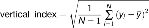where N is the number of root pixels, x_i are the x-coordinates of the root pixels, and y_i are the y-coordinates of the root pixels. The root linearity is the coefficient of linear determination (R²) of the linear regression line fitted to the pixels of the primary root skeleton using the method of least squares. A value near 1 would mean that the root could be approximated by a straight line, while a low value stands for a curved or wavy root. The root width is calculated by determining the distance map of the root pixels and is therefore proportional to the root diameter. It is calculated in different longitudinal zones of the root. The average root width denotes the root width averaged over all root pixels. Additionally, the root widths over intervals or longitudinal zones are calculated. “Root Width 20” denotes the mean value for the section from 0 to 20% of the total root length starting at the hypocotyl-root junction point. “Root Width [40, 60, 80, 100]” are similar values for the sections 20 to 40%, 40 to 60%, 60 to 80%, or 80 to 100% of the total root length, respectively.

File Output

BRAT generates multiple files. The segmentation step writes a file containing the basic measurements of root and shoot objects. In the postprocessing step in which the user provides the genotype layout file (Supplemental Table 1), these measurements are used in the calculations where averages, medians, and various combinations of different traits are derived. The calculations are done on a per-plant basis and on a per-accession basis. For each calculation, the number of involved individuals and the standard variations for the traits are saved. This enables the user to filter underpopulated or high-variation subsets.

Root Width Determination Using Confocal Microscopy

An LSM 700 Axio Observer.Z1 confocal microscope (Zeiss) with a motorized stage was used for confocal image acquisition. Plants grown on agar plates that had been measured using BRAT were incubated with 20 μg/mL propidium iodide for 10 s, washed in monoQ water, transferred to standard microscopy slides, and mounted in monoQ water. Using a 2.5× dry objective (Zeiss Fluar 2.5×/0.12 numerical aperture), an overview image of the each complete root was acquired using the tile scan function (3 × 5 tiles) of ZEN2010 software and with a resolution of 6.252 μm/pixels. Propidium iodide was excited at 488 nm with full laser power and detected at 576 to 700 nm. The focus was set at the medial longitudinal section in the estimated interval of interest. After image acquisition, the root length was measured using the manual segmentation tool in Fiji and divided into five intervals (the same intervals as for the width trait measurements using BRAT). Within the interval of interest (20 to 40% of root length starting from the hypocotyl/root boundary), the root width was measured on the images manually in Fiji at three points that would correspond to 20, 30, and 40% of root length. Finally, the average value was calculated to obtain the three-point average root width estimation for 20 to 40% interval of root length.

Performance Evaluation

The evaluation of the high-throughput software performance was based on the same five images containing plants grown from 120 seeds (n = 118). Image formats and resolution were modified according to software specifications and to allow for good performance of the evaluated software.

Robustness Assay

To evaluate BRAT robustness toward various experimental conditions, we used seven different conditions that possibly alter the background, contrast, or root growth direction. These were sulfur deficient, iron deficient, phosphorus deficient, low pH, low temperature (10°C), high temperature (29°C), and auxin transport inhibitor 1-N-naphtylphthalamic acid (10 μM) supplemented plates. Nutrient deficiency media were prepared as described (Iyer-Pascuzzi et al., 2011). Evaluation was done on four whole plate images containing plants grown from 96 seeds at day 3 after germination for all but one condition and at day 15 after plating in the case of low temperature.

Genome-Wide Association Mapping

We used the average trait value for 78 traits of 163 accessions quantified by BRAT (n = 5 to 24) to conduct GWA using an accelerated mixed model (EMMAX) (Kang et al., 2010) followed by EMMA (Kang et al., 2008) for the most significant 200 associations. The GWA was performed on a cluster, with algorithms identical to the ones used in the GWAPP Web interface (Seren et al., 2012). SNPs with minor allele counts greater or equal to 12 were taken into account. The significance of SNP associations was determined at 5% FDR threshold computed by the Benjamini-Hochberg-Yekutieli method to correct for multiple testing (Benjamini and Hochberg, 1995).

Analyses of Allelic variation

We used the 215K SNP data to extract the SNP alleles for the top association (chromosome 5; position 7738620). We mapped these alleles using the GPS coordinates of the accessions on the BioClim Bio11 map (Kriticos et al., 2012) using QGIS 2.2 (http://www.qgis.org/). The visual maps were created using the QGIS OpenLayers plug-in and by obtaining a Google Physical Maps layer. We calculated the distance of the accessions to the closest coordinate of the ocean using the Proximity (Raster Distance) function of QGIS. We then extracted the distance values using the point sampling tools of QGIS. Due to the BioClim map resolution, the accuracy of the positions is around 18 km. A shift of the distribution of the distances of the accessions with the major SNP allele on chromosome 5 at position 7738620 (“T”) to the distribution of the minor SNP allele (“A”) was tested using a two-tailed Wilcoxon rank sum test with continuity correction (Hollander and Wolfe, 1973) in R 3.0.2 (http://www.r-project.org/) using the wilcox.test function.

The selection scan data were obtained using the Arabidopsis Selection Browser (http://regmap.uchicago.edu/cgi-bin/gbrowse/arabidopsis/).

Accession Numbers

Sequence data from this article can be found in The Arabidopsis Information Resource and GenBank (National Center for Biotechnology Information) databases under the following accession numbers: CaS (AT5G23060) and the list of gene identifier numbers in Supplemental Data Set 1.

Supplemental Data

The following materials are available in the online version of this article.

• Supplemental Figure 1. Detection of the Plate’s Area.

• Supplemental Figure 2. Plant and Shoot Detection Algorithms of BRAT.

• Supplemental Figure 3. Screenshot of the Optional BRAT Quality Control Interface.

• Supplemental Figure 4. Correlation of Root Width Measurements: BRAT vs. Confocal Microscopy.

• Supplemental Figure 5. Performance of BRAT under Various Experimental Conditions.

• Supplemental Figure 6. Example Images of the Roots and Trait Values for Extreme Accessions for Relative Root Growth Rate.

• Supplemental Figure 7. Abundance of CaS (AT5G23060) Transcript in the Root.

• Supplemental Figure 8. Effects of Loss of Function and Overexpression of CaS Gene on Primary Root Length on Agar Plates.

• Supplemental Figure 9. Worldwide Distribution of Alleles for Top CaS SNP and Signs of Selection at CaS Genomic Locus.

• Supplemental Figure 10. Grid Layout Template and Positional Permutations.

• Supplemental Figure 11. Microscope Calibration Slide.

• Supplemental Figure 12. The Naming Pattern Supported by BRAT.

• Supplemental Figure 13. Illustration of Root Angle Trait.

• Supplemental Figure 14. Calculation of Root Direction Index.

• Supplemental Table 1. Genotype Layout File.

• Supplemental Table 2. Time Requirements of High-Throughput Root Phenotyping Software Tools.

• Supplemental Table 3. 163 Accessions Used in This Study.

• Supplemental Data Set 1. Significant SNPs from Genome-Wide Association Studies.

Glossary

GWA

genome-wide association

GUI

graphical user interface

MP

megapixel

ROI

region of interest

QC

quality control

GWAS

genome-wide association study

FDR

false discovery rate

SNP

single nucleotide polymorphism

MS

Murashige and Skoog

References

- Alonso J.M., et al. (2003). Genome-wide insertional mutagenesis of Arabidopsis thaliana. Science 301: 653–657. [DOI] [PubMed] [Google Scholar]
- Armengaud P., Zambaux K., Hills A., Sulpice R., Pattison R.J., Blatt M.R., Amtmann A. (2009). EZ-Rhizo: integrated software for the fast and accurate measurement of root system architecture. Plant J. 57: 945–956. [DOI] [PubMed] [Google Scholar]
- Atwell S., et al. (2010). Genome-wide association study of 107 phenotypes in Arabidopsis thaliana inbred lines. Nature 465: 627–631. [DOI] [PMC free article] [PubMed] [Google Scholar]
- Baxter I., Brazelton J.N., Yu D., Huang Y.S., Lahner B., Yakubova E., Li Y., Bergelson J., Borevitz J.O., Nordborg M., Vitek O., Salt D.E. (2010). A coastal cline in sodium accumulation in Arabidopsis thaliana is driven by natural variation of the sodium transporter AtHKT1;1. PLoS Genet. 6: e1001193. [DOI] [PMC free article] [PubMed] [Google Scholar]
- Benjamini Y., Hochberg Y. (1995). Controlling the false discovery rate - a practical and powerful approach to multiple testing. J. Roy. Stat. Soc. B Met. 57: 289–300. [Google Scholar]
- Brady S.M., Orlando D.A., Lee J.Y., Wang J.Y., Koch J., Dinneny J.R., Mace D., Ohler U., Benfey P.N. (2007). A high-resolution root spatiotemporal map reveals dominant expression patterns. Science 318: 801–806. [DOI] [PubMed] [Google Scholar]
- Brady S.M., et al. (2011). A stele-enriched gene regulatory network in the Arabidopsis root. Mol. Syst. Biol. 7: 459. [DOI] [PMC free article] [PubMed] [Google Scholar]
- Breakfield N.W., Corcoran D.L., Petricka J.J., Shen J., Sae-Seaw J., Rubio-Somoza I., Weigel D., Ohler U., Benfey P.N. (2012). High-resolution experimental and computational profiling of tissue-specific known and novel miRNAs in Arabidopsis. Genome Res. 22: 163–176. [DOI] [PMC free article] [PubMed] [Google Scholar]
- Clark R.T., Famoso A.N., Zhao K., Shaff J.E., Craft E.J., Bustamante C.D., McCouch S.R., Aneshansley D.J., Kochian L.V. (2013). High-throughput two-dimensional root system phenotyping platform facilitates genetic analysis of root growth and development. Plant Cell Environ. 36: 454–466. [DOI] [PubMed] [Google Scholar]
- Clough S.J., Bent A.F. (1998). Floral dip: a simplified method for Agrobacterium-mediated transformation of Arabidopsis thaliana. Plant J. 16: 735–743. [DOI] [PubMed] [Google Scholar]
- Danielsson P.E. (1980). Euclidean distance mapping. Comput. Graphics Image Process. 14: 227–248. [Google Scholar]
- Dijkstra E.W. (1959). A note on two problems in connexion with graphs. Numer. Math. 1: 269–271. [Google Scholar]
- Dinneny J.R., Long T.A., Wang J.Y., Jung J.W., Mace D., Pointer S., Barron C., Brady S.M., Schiefelbein J., Benfey P.N. (2008). Cell identity mediates the response of Arabidopsis roots to abiotic stress. Science 320: 942–945. [DOI] [PubMed] [Google Scholar]
- French A., Ubeda-Tomás S., Holman T.J., Bennett M.J., Pridmore T. (2009). High-throughput quantification of root growth using a novel image-analysis tool. Plant Physiol. 150: 1784–1795. [DOI] [PMC free article] [PubMed] [Google Scholar]
- Guan Q., Wu J., Yue X., Zhang Y., Zhu J. (2013). A nuclear calcium-sensing pathway is critical for gene regulation and salt stress tolerance in Arabidopsis. PLoS Genet. 9: e1003755. [DOI] [PMC free article] [PubMed] [Google Scholar]
- Hollander, M., and Wolfe, D.A. (1973). Nonparametric Statistical Methods. (New York: Wiley). [Google Scholar]
- Horton M.W., et al. (2012). Genome-wide patterns of genetic variation in worldwide Arabidopsis thaliana accessions from the RegMap panel. Nat. Genet. 44: 212–216. [DOI] [PMC free article] [PubMed] [Google Scholar]
- Iyer-Pascuzzi A.S., Jackson T., Cui H., Petricka J.J., Busch W., Tsukagoshi H., Benfey P.N. (2011). Cell identity regulators link development and stress responses in the Arabidopsis root. Dev. Cell 21: 770–782. [DOI] [PMC free article] [PubMed] [Google Scholar]
- Kang H.M., Sul J.H., Service S.K., Zaitlen N.A., Kong S.Y., Freimer N.B., Sabatti C., Eskin E. (2010). Variance component model to account for sample structure in genome-wide association studies. Nat. Genet. 42: 348–354. [DOI] [PMC free article] [PubMed] [Google Scholar]
- Kang H.M., Zaitlen N.A., Wade C.M., Kirby A., Heckerman D., Daly M.J., Eskin E. (2008). Efficient control of population structure in model organism association mapping. Genetics 178: 1709–1723. [DOI] [PMC free article] [PubMed] [Google Scholar]
- Kobayashi Y., Hoekenga O.A., Itoh H., Nakashima M., Saito S., Shaff J.E., Maron L.G., Piñeros M.A., Kochian L.V., Koyama H. (2007). Characterization of AtALMT1 expression in aluminum-inducible malate release and its role for rhizotoxic stress tolerance in Arabidopsis. Plant Physiol. 145: 843–852. [DOI] [PMC free article] [PubMed] [Google Scholar]
- Kriticos D.J., Webber B.L., Leriche A., Ota N., Macadam I., Bathols J., Scott J.K. (2012). CliMond: global high-resolution historical and future scenario climate surfaces for bioclimatic modelling. Methods Ecol. Evol. 3: 53–64. [Google Scholar]
- Land K., Slosar A., Lintott C., Andreescu D., Bamford S., Murray P., Nichol R., Raddick M.J., Schawinski K., Szalay A., Thomas D., Vandenberg J. (2008). Galaxy Zoo: the large-scale spin statistics of spiral galaxies in the Sloan Digital Sky Survey. Mon. Not. R. Astron. Soc. 388: 1686–1692. [Google Scholar]
- Laohavisit A., Richards S.L., Shabala L., Chen C., Colaço R.D., Swarbreck S.M., Shaw E., Dark A., Shabala S., Shang Z., Davies J.M. (2013). Salinity-induced calcium signaling and root adaptation in Arabidopsis require the calcium regulatory protein annexin1. Plant Physiol. 163: 253–262. [DOI] [PMC free article] [PubMed] [Google Scholar]
- Lloyd A.M., Barnason A.R., Rogers S.G., Byrne M.C., Fraley R.T., Horsch R.B. (1986). Transformation of Arabidopsis thaliana with Agrobacterium tumefaciens. Science 234: 464–466. [DOI] [PubMed] [Google Scholar]
- Lobet G., Pagès L., Draye X. (2011). A novel image-analysis toolbox enabling quantitative analysis of root system architecture. Plant Physiol. 157: 29–39. [DOI] [PMC free article] [PubMed] [Google Scholar]
- Lorensen W.E., Cline H.E. (1987). Marching cubes: A high resolution 3D surface construction algorithm. SIGGRAPH Comput. Graph. 21: 163–169. [Google Scholar]
- Lowe D.G. (2004). Distinctive image features from scale-invariant keypoints. Int. J. Comput. Vis. 60: 91–110. [Google Scholar]
- Meijón M., Satbhai S.B., Tsuchimatsu T., Busch W. (2014). Genome-wide association study using cellular traits identifies a new regulator of root development in Arabidopsis. Nat. Genet. 46: 77–81. [DOI] [PubMed] [Google Scholar]
- Monshausen G.B., Miller N.D., Murphy A.S., Gilroy S. (2011). Dynamics of auxin-dependent Ca2+ and pH signaling in root growth revealed by integrating high-resolution imaging with automated computer vision-based analysis. Plant J. 65: 309–318. [DOI] [PubMed] [Google Scholar]
- Nomura H., Komori T., Kobori M., Nakahira Y., Shiina T. (2008). Evidence for chloroplast control of external Ca2+-induced cytosolic Ca2+ transients and stomatal closure. Plant J. 53: 988–998. [DOI] [PubMed] [Google Scholar]
- Petricka J.J., Schauer M.A., Megraw M., Breakfield N.W., Thompson J.W., Georgiev S., Soderblom E.J., Ohler U., Moseley M.A., Grossniklaus U., Benfey P.N. (2012). The protein expression landscape of the Arabidopsis root. Proc. Natl. Acad. Sci. USA 109: 6811–6818. [DOI] [PMC free article] [PubMed] [Google Scholar]
- Pierret A., Gonkhamdee S., Jourdan C., Maeght J.L. (2013). IJ_Rhizo: an open-source software to measure scanned images of root samples. Plant Soil 373: 531–539. [Google Scholar]
- Ridler T.W., Calvard S. (1978). Picture thresholding using an iterative selection method. IEEE T. Syst. Man. Cyb. 8: 630–632. [Google Scholar]
- Ryser P. (2006). The mysterious root length. Plant Soil 286: 1–6. [Google Scholar]
- Schindelin J., et al. (2012). Fiji: an open-source platform for biological-image analysis. Nat. Methods 9: 676–682. [DOI] [PMC free article] [PubMed] [Google Scholar]
- Seren Ü., Vilhjálmsson B.J., Horton M.W., Meng D., Forai P., Huang Y.S., Long Q., Segura V., Nordborg M. (2012). GWAPP: a web application for genome-wide association mapping in Arabidopsis. Plant Cell 24: 4793–4805. [DOI] [PMC free article] [PubMed] [Google Scholar]
- Vainonen J.P., Sakuragi Y., Stael S., Tikkanen M., Allahverdiyeva Y., Paakkarinen V., Aro E., Suorsa M., Scheller H.V., Vener A.V., Aro E.M. (2008). Light regulation of CaS, a novel phosphoprotein in the thylakoid membrane of Arabidopsis thaliana. FEBS J. 275: 1767–1777. [DOI] [PubMed] [Google Scholar]
- Xu G.Y., Rocha P.S., Wang M.L., Xu M.L., Cui Y.C., Li L.Y., Zhu Y.X., Xia X. (2011). A novel rice calmodulin-like gene, OsMSR2, enhances drought and salt tolerance and increases ABA sensitivity in Arabidopsis. Planta 234: 47–59. [DOI] [PubMed] [Google Scholar]
- Zhang T.Y., Suen C.Y. (1984). A fast parallel algorithm for thinning digital patterns. Commun. ACM 27: 236–239. [Google Scholar]
Associated Data
This section collects any data citations, data availability statements, or supplementary materials included in this article.