Abstract
In this work we discuss a spatial evolutionary model for a heterogeneous cancer cell population. We consider the gain-of-function mutations that not only change the fitness potential of the mutant phenotypes against normal background cells but may also increase the relative motility of the mutant cells. The spatial modeling is implemented as a stochastic evolutionary system on a structured grid (a lattice, with random neighborhoods, which is not necessarily bi-directional) or on a two dimensional unstructured mesh, i.e. a bi-directional graph with random numbers of neighbors. We present a computational approach to investigate the fixation probability of mutants in these spatial models. Additionally, we examine the effect of the migration potential on the spatial dynamics of mutants on unstructured meshes. Our results suggest that the probability of fixation is negatively correlated with the width of the distribution of the neighborhood size. Also, the fixation probability increases given a migration potential for mutants. We find that the fixation probability (of advantaged, disadvantaged and neutral mutants) on unstructured meshes is relatively smaller than the corresponding results on regular grids. More importantly, in the case of neutral mutants the introduction of a migration potential has a critical effect on the fixation probability and increases this by orders of magnitude. Further, we examine the effect of boundaries and as intuitively expected, the fixation probability is smaller on the boundary of regular grids when compared to its value in the bulk. Based on these computational results, we speculate on possible better therapeutic strategies that may delay tumor progression to some extent.
Keywords: Math Oncology, Random Meshes, Cell Migration, Cellular Automata, Evolutionary Modeling
1. Introduction
Cancer can be viewed as an evolutionary process, where a collection of pre-neoplastic clones acquire genetic and epigenetic changes over a period of time [1]. During the process of carcinogenesis, it is commonly believed that mutant cells with a gain-of-function fitness advantage take over a small neighborhood of host cells through a selection process and initiate a clonal area, leading to invasion into the proximal tissue. The fitness rates of preneoplastic clones are effected by a mutation-selection mechanism and various micro-environmental factors, and as a result a growing tumor has a high level of heterogeneity at the cellular level. Both initiation and progression stages have been proposed to follow an evolutionary stochastic model and different authors have observed the effect of a fitness advantaged mutant introduced into the system and the probability that this takes over a finite compartment of the cellular tissue. In recent years (see [2]–[9]), these models have been successfully applied to both one-hit and two-hit mutation-selection processes. During the final stages of malignancy, the mutant phenotype gains a relative advantage through motility. The evolutionary theory of these complex phenomena has not yet been addressed in the literature.
For the past three decades, there have been several attempts to understand the process of fixation in spatially homogeneous systems. It was found that many spatially structured models such as lattices models have little or no effect on the selection process [10]–[13]. More recently, Lieberman et al [14] generalized this to arbitrary graphs and found the exact symmetry conditions under which the fixation probability for an advantaged mutant, evolving on a graph, is the same as that for a mixed population model. Houchmandzadeh et al [15] demonstrated that fixation probability of a beneficial mutation in a geographically structured population is almost the same (or, slightly smaller) compared to the unstructured population for a Voter framework.
Many authors have studied the spatial dynamics of cancer invasion using cellular automata/ agent based models, partial differential equation models, and hybrid models including multiscale modeling techniques [16]—[36]. In these models, it is possible to incorporate progressively more complex cellular mechanisms and biological phenomena [20]. In the current paper, we adopt a simpler approach. In an attempt to understand and analyze the dynamics of invasion, we focus on only two forces, namely, proliferative and migrative potentials that influence the inherited genetic behavior of mutants.
Our approach builds on spatial evolutionary modeling of cancer initiated in [6], where the process was described as a linear chain (1D). In this spatial model, cells were placed linearly at different positions, and restricted to replicate only to a neighboring point after a cell death. In this model, the fixation probability of single hit and double hit mutants was investigated. In particular, it was found that in the spatial case, the probability of fixation of advantaged and disadvantaged single mutants is lower compared to that in the space-free model. An extension of this 1D model is presented in [8], where the spatial dynamics on a 2D lattice is analyzed. Two genetic factors are considered: replicative potential and cellular motility. The overall conclusion is that migration has a major impact on the probability of a single mutant cell's ability to invade an existing colony, something that had not been investigated in previous modeling efforts to understand cancer progression.
The goal of the present study is to develop a better quantitative analysis of the invasion probability, by avoiding the rigid framework imposed by a regular grid. We introduce a stochastic death-birth model (i.e., the Moran process [37]) for the spatial evolutionary system. In order to circumvent the rigidity of a regular grid, we use two different methods. In the first construction, we start with a regular square lattice and add/remove neighbors in a random way (the background lattice can be of Moore neighborhood type with 8 neighbors, or, von-Neumann neighborhood, with 4 neighbors). The important feature of this construction of the connectivity graph is the notion that we construct the number of neighbors for each of the nodes on the lattice (where each node is occupied by either a normal or a mutant cell). This construction is a mixture of both directed and undirected links, i.e., some nodes and their neighbors are bi-directional and some are uni-directional.
Broadly speaking, any regular grid assumes that the number of neighbors around each cell is homogeneous at every location in space. This is not a realistic assumption for modeling biological tissues. An unstructured mesh where the number of neighbors around each nodal position is a random variable, can be a better approximation to reality. This suggests our second construction, where we consider an unstructured mesh which is defined as a random neighborhood graph with longer ranges of connectivities versus the previous case. The distinguishing feature however, is the main fact that the unstructured mesh does behave symmetrically between the two type of species in terms of the connectivity graph and the number of neighbors. The contrasting feature in the unstructured mesh construction is that every node and its corresponding neighbors are bi-directional compared to the previous scenario.
Here, we are mainly concerned with the question of fixation probability in the presence of a migration potential, or cellular motility for either only the mutant phenotype or for both the normal and mutant phenotypes. We address the effects of a random environment and migration potential on the fixation probability.
The paper is organized as follows. In Sec. 2 we review the background related to space free and spatial models, and introduce our spatial model in the presence of a migration potential/motility. In Sec. 3 we investigate the two spatial models of structured grids with variable (static and dynamic) neighborhoods and observe the effect of varying the number of neighbors and/or migration potentials of both cell types. We subsequently turn to the unstructured mesh to investigate the effect of migration potential on the fixation probability. The effect of boundaries on the value of the fixation probability is briefly discussed at the end of Sec. 3. We discuss the biological relevance and connections to the known analytical limits of the models in the discussion part, Sec. 4.
2. Methods
2.1. Background
The traditional Moran process is described as follows. Consider a population of N cells consisting of two phenotypes: A (host cells) and B (mutant cells). We also refer to type B cells as pre-cancerous or pre-malignant cells throughout the paper. Each cell type has a proliferative potential. At every time step, one cell is randomly chosen for death and is replaced by the progeny of another randomly chosen cell from the same population, such that the population size is constant at every time step. Cells are chosen for death with equal probabilities, and they are chosen to reproduce according to their relative fitness. We assume that the two cell types A and B have fitness rates rA = 1 and rB = r respectively. If the number of B cells is i, then the probability that B is chosen for reproduction is PB+ = ri/(N −i+ri). The Moran process is a one-dimensional birth-death process which tracks the number of type B cells over time. Its properties in the context of invasion probability and other statistical features have been discussed in detail in [2]—[15].
A spatial generalization of the above model is considered as a 1D model in [6], in which a population of N cells are placed along a line at locations 1, 2, . . . , N. As before, at each time-step a cell is randomly chosen for death, and the empty spot is subsequently occupied by the progeny of one of the two neighboring cells, proportional to their fitness.
A second generalization of this model is introduced in [8], where a population of N cells consisting of cells of types A and B, is placed on a rectangular grid (such that all grid points are filled). Both division and migration potentials of A and B cells are incorporated in the model dynamics. Let rA and rB be the division rates and mA and mB the migration rates of type A and B cells respectively. Each update starts off with a cell chosen randomly to die. Then one of the following four events might occur: A divides, B divides, A migrates, B migrates. If a division event of A or B occurs, then the update is complete and the process is repeated again. If a migration event occurs, then the empty spot is occupied by a migratory cell, leaving another empty spot behind. Again, a new elementary event is considered till the empty spot is filled (i.e. until the occurrence of a division event). The grid is always filled up at the end of each update following the Moran process assumption that the whole population is constant at every iteration.
The model chooses the nearest neighbors around the empty spot taken to be a von-Neumann neighborhood (i.e. four neighbors). Suppose nA and nB are the number of type A and B cells around the empty spot, then the probabilities of each elementary event are given by
| (1) |
| (2) |
| (3) |
| (4) |
where Δ = nA(rA+mA)+nB(rB+mB). Introducing dimensionless variables, equations (1)–(4) can be rewritten as:
| (5) |
| (6) |
| (7) |
| (8) |
where λ = rB/rA, with kX = mX/rX (for X = A, B). For the spatial model outlined above, the simulations in [8] were performed on a square grid with periodic boundary conditions.
3. The effect of variable neighborhoods
It is clearly evident that equations (1)–(4) are dependent on the number of neighboring cells of type A and B, which is fixed in the approach described in [8]. We now generalize the above expressions to include random sets of neighbors at each nodal position. This leads to changes in nA and nB that in turn might affect the cellular dynamics of the whole system. We explore the possible consequences of this change in two different numerical experiments. We apply the algorithm outlined above for all the computations in this work by running 5 sets of simulations of 10000 iteration each, and each iteration is performed until, for a fixed neighborhood, the system reaches fixation and we estimate the invasion probability. The uncertainty is obtained using the definition of standard deviation and plotted along with the mean.
3.1. Regular mesh, random neighborhoods
The isothermal theorem for graphs [14] states that, if each node of a graph has the same number of neighboring nodes, i.e. a symmetric bidirectional graph, then the invasion probability is equivalent to that of the fixation probability of the traditional Moran process in the absence of migration. Thus the invasion probability obtained from symmetric graphs provides no further insight into the complex features of the tissue architecture. As a result of this, we examine the variation in the invasion probability for two different scenarios by introducing randomness so that it specifically introduces asymmetry into the problem despite the symmetry of the graph.
Static Random Neighborhoods
In the first scenario, we investigate the invasion dynamics resulting from a random number of neighbors chosen from a fixed distribution at each node on a regular lattice. This simulation is carried out by fixing the mean number of neighbors and varying the width of the distribution. The neighborhood size for each grid point is assumed to be a random, integer-valued variable distributed uniformly over a given interval. We varied this distribution from a delta-function to a distribution with a relatively wide spread. This experiment was carried out to investigate the correlation between the invasion probability and the distribution width. We considered a regular, square lattice comprised of 21 × 21 = 441 cells with reflecting boundary conditions. Random numbers of neighbors are generated from a uniform distribution, in such a way that the average number of neighbors is always 4, but the width varies.
The algorithm used for the experiments can be summarized as follows. The following construction is carried out such that the delta distribution follows a background mesh, i.e., a lattice with four neighbors. For each nodal point on the grid, we generate a random number of neighbors from a given distribution, say D = [1, 7]. The number of neighbors for each node will then be 1, 2, . . . , or, 7. Then, distances are computed from every node to all other nodes on the lattice. The nearest set of neighbors for a particular node is then considered depending on the nodes that are located closest. If two or more nodes are located at the same distance from the given node, then we randomly pick a node. This construction introduces a mixture of both directed and undirected connections between a node and its neighbors (i.e. some nodes and their neighbors may be symmetric, while others will be asymmetric). The set of neighbors generated for each node on the lattice is fixed throughout the experiment.
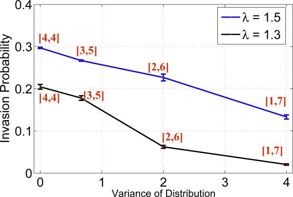
For a distribution with zero width (on a lattice), the invasion probability of the mutant highly depends on its migration and reproductive potentials. Simulations were carried out by applying the algorithm outlined in the previous section with reflecting boundary conditions for advantaged mutants. We obtain a similar figure with approximate values of invasion probability captured in Figure 1 in the paper [8]. Also, if the number of neighbors is uniformly increased or decreased, i.e., each node still consists of the same number of neighbors, we can intuitively assume that this may not change the invasion probability.
Figure 1.
Invasion probability of mutants as a function of varying distribution width with static random neighborhood in a migration free system. Parameters: lattice size = 21 × 21, λ = 1.5, 1.3, kA = kB = 0.
Now, we introduce a variation on the number of neighbors at each nodal position, which can be attributed to the asymmetry of the lattice.
At the start of each simulation one mutant is introduced at a randomly chosen position in the lattice, where the remaining cells populating the lattice are type A cells. Simulations are run, and each iteration is performed until, for a fixed neighborhood, the system reaches fixation and we estimate the invasion probability.
In the first scenario, simulations were carried out for advantaged mutants (λ = 1.5) assuming zero migration for both types of cells. The effect of the width of the distribution on the invasion probability is captured in Figure 1 for a migration free system. It is clearly evident that the invasion probability decreases with the width of the distribution.
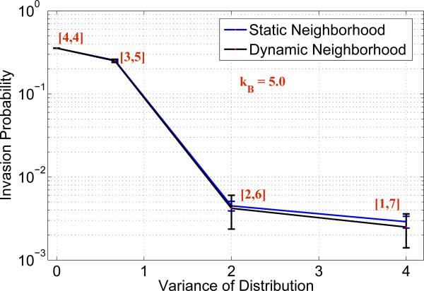
Secondly, the simulations were run only for advantaged mutants (λ = 1.5) assuming the migration of A cells is zero, i.e. kA = 0. This experiment is done in order to understand the effect of migration on the invasion probability. The effect of the width of the distribution on the invasion probability is plotted in Figure 2, where zero width corresponds to the results reported in [8]. From the figure, we clearly observe that the invasion probability is negatively correlated with the width of the distribution, i.e., as we increase the width of the distribution the invasion probability decreases. In the presence of migration which is captured in Figure 2, we do not observe a significant change in the invasion probability for the distribution [3, 5] compared with a migration free system. However, for distributions [2, 6] and [1, 7], migration suppresses the invasion probability, due to the chaotic architecture. The invasion probability drops to the order of 10−3 when neighbors are selected from the distribution [1, 7].
Figure 2.
Invasion probability of mutants as a function of varying distribution width with static and dynamic random neighborhood. Parameters: lattice size = 21 × 21, λ = 1.5, kB = 5.0 and kA = 0.
The invasion probability decreases with increasing distribution width. The randomness of the architecture pushes the generated random mesh far away from the isothermal graph (whose invasion probability is equivalent to that of the Moran process fixation probability). This has been earlier studied on scale free networks [38]. For a high variance of the distribution of neighbors, we can possibly have several clusters of cells which are very poorly connected to each other (due to the unidirectional construction of the random mesh). These poorly connected clusters increase as the variance increases, leading to mutant extinction implying a smaller invasion probability.
Dynamic random neighborhoods
The second experiment is similar to the one described above, except that we generate a new random set of neighbors at every iteration. This experiment is carried out to examine the effect of the change in tissue geometry after every iteration. Simulations were run, and each iteration is performed until, for a fixed initial neighborhood, the system reaches fixation and we estimate the invasion probability. The effect of the width of the distribution on the invasion probability is similar to the plot presented in Figure 1 for a migration free environment (because, averaging over a dynamic random neighborhood gives a static random neighborhood). To observe the effect of migration of B cells on the invasion probability, we assumed the migration potential of A cells to be zero, i.e. kA = 0. The simulations were run only for advantaged mutants (λ = 1.5), kB = 5.0, and the invasion probability is computed for varying distribution widths is presented in Figure 2.
In the first experiment (static neighborhood), the number of neighbors are static throughout the whole set of iterations, which can be thought of as a fixed set of neighborhood clusters over time for every node. However, in the second experiment (dynamic neighborhood) the number of neighbors changes for every iteration, i.e., this can be understood as the change in the neighborhood size over time. In order to appreciate the effect of the distribution width on the invasion probability, consider the following comparison. For simplicity, let us take kA = kB = 0, a case of no migration. In the case of the lattice model with a fixed grid (which corresponds to the zero-width distribution, [4, 4]), the invasion probability of an advantageous mutant with λ = 1.5 is given by 0.2969. When we use a random neighborhood model and increase the distribution width to that of [2, 6], the fixation probability drops to 0.2267. This clearly indicates that for a migration free system, proliferative potential is hindered due to the increase in the width of the distribution, thereby decreasing the invasion probability. Another interesting observation from Figure 2 is that, we notice that for the distribution [1, 7] the invasion probability is close (i.e., of the same order) to the invasion probability of a neutral mutant (which is given by ρneutral = 1/N = 0.0022). This suggests that an increase in the distribution width can eliminate the advantage given by a 50% increase in the replication potential. By increasing the width of the distribution, the invasion probability decreases rapidly and approaches the invasion probability of mutants with neutral drift, which is strongly suggested from a study of lower and upper bounds of fixation probabilities on a graph [39].
From the biological point of view, the alterations in the neighborhood for each node can be attributed to tension, stress, and several other micro-environmental factors. These results strongly suggest that the geometry of the neighborhood (either static/dynamic) plays an important role in the invasion probability under constrained boundaries, both in a migration free system as well as in the presence of migration.
3.2. Unstructured mesh
Next, the invasion dynamics of pre-cancerous cells is explored on an unstructured mesh. The construction of an unstructured (or, a Voronoi) mesh is completely different from the construction of the static and random neighborhood lattices in Sec. 3.1. An unstructured mesh is constructed using QHull in Matlab software. In the static and random neighborhood scenarios, the links or connections between a node and its neighbors are either unidirectional or bi-directional; however, in the case of unstructured meshes the links between a node and its neighbors are bidirectional. It is well known that on an unstructured grid, the number of neighbors at each location can vary greatly. The impact of the migration potential on the invasion probability is analyzed and compared with the corresponding results on a regular grid structure for two different scenarios. In the first scenario we assume that the migration potential of B (or mutant) cells is kB > 0 and the migration ability of A cells is chosen to be kA = 0. In the second scenario we consider migration potentials of both types of cells to be kA, kB > 0.
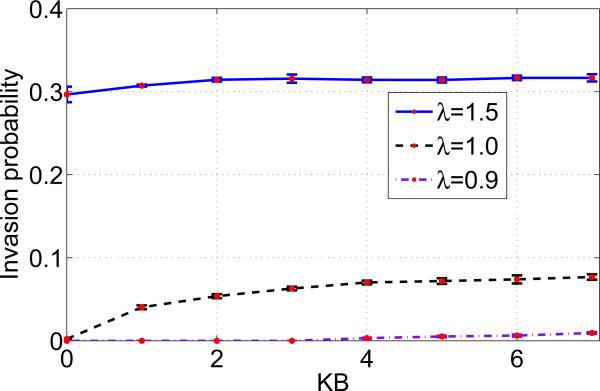
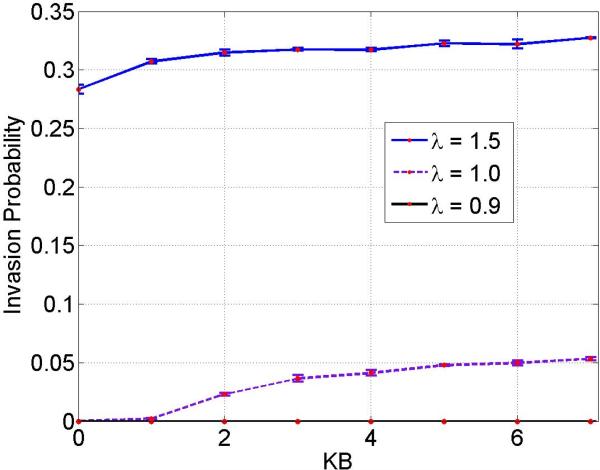
Randomly, one mutant (type B) cell is introduced into the mesh whilst the rest of the cells populating the mesh are type A cells. Our system is now composed of N − 1 type A or host cells and a single mutant or type B cell. The algorithm outlined in the previous sections is applied with reflecting boundary conditions, again until one of the cell types becomes extinct. For all three cases of mutants, we observed that the invasion probability is much smaller when compared to the corresponding results on a lattice. Figure 3 is a plot of the invasion probability against the migration potential of type B cells assuming zero migration potential for type A cells, kA = 0. We ran the simulations for advantaged mutants (λ = 1.5), neutral mutants (λ = 1.0) and disadvantaged mutants (λ = 0.9) and the effect of the migration potential on the invasion probability is plotted for each kB. Simulations are run, and each iteration is performed until, for a fixed initial neighborhood, the system reaches fixation and we estimate the invasion probability.
Figure 3.
Invasion probability of various mutants as a function of migration potential of type B mutant on an Unstructured mesh. Parameters: mesh size = 441 elements, λ = 1.5, 1.0, 0.9 and kA = 0.
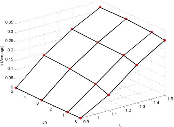
We then changed the values of λ for several migration potentials kB, and plotted these against the average invasion probability. A contour plot is presented in Figure 4, clearly indicating that the proliferative potential plays an important role along with the migration potential. Another interesting feature worth highlighting is that, for a fixed migration potential and varying proliferative potential, the invasion probability increases almost linearly.
Figure 4.
Contour plot of average invasion probability of various mutants against migration potential of type B mutant and proliferative potentials λ on an Unstructured mesh. Parameters: mesh size = 441 elements and kA = 0.
Figure 5 displays the invasion probability against the migration potential of type B cells assuming that the migration potential of type A cells is non zero, kA > 0. The simulations were run for advantaged mutants (λ = 1.5), neutral mutants (λ = 1.0) and disadvantaged mutants (λ = 0.9). A significant change was not observed in the invasion probabilities of mutants with either zero or non zero (and lower) migration potential of type A cells (results not shown here). This indicates that lower migration potentials of type A cells does not have a predominant impact on invasion.
Figure 5.
Invasion probability of various mutants as a function of migration potential of type B mutant on an Unstructured mesh. Parameters: mesh size = 441 elements, λ = 1.5, 1.0, 0.9 and kA = 1. Notice that invasion probability is very small when kB ≤ kA, and it is also vanishingly small in the case of disadvantaged mutant λ = 0.9.
From Figures 3 and 5, we observe that in the absence of migration, i.e. when kA = 0 and kB = 0, the invasion probability which is 0.2969 is close to the fixation probability of the classical Moran process 0.3333. The small change can be attributed to either computational errors or to the geometry of the mesh. Also, the nodes located at the boundary may play an important role because of lesser number of neighbors (which can be interpreted as links/connections) associated with these. Another interesting observation is with respect to the neutral drift of mutants. In Figures 3 and 5, for the scenario λ = 1.0, i.e., rA = rB and for kA = kB, the invasion probability is almost equivalent to (i.e., is of the same order as) the fixation probability for a system (in the absence of boundary effects) with neutral drift which is ρneutral drift = 1/N = 0.0022. From Figure 5, the change in the invasion probability is clearly observed around the point kA = kB = 1.0, for a neutral mutant (i.e., λ = 1.0). We observe the two regimes for a neutral mutant, i.e kB < 1.0 and kB > 1.0 . For kB < 1.0, the invasion probability is very small and close to zero, while we observe a non-zero invasion probability in the regime kB > 1.0 . Thus, the change in the invasion probability is around neutral mutant.
The aforementioned change can be attributed to the asymmetric nature of migration rates between type A and B cells. This suggests strongly that migration does affect the system unless there is a higher rate of migration advantage to the mutant cell as compared to the host cell. The invasion probability is vanishingly small for disadvantaged mutants in the presence of migration of type A cells, which is captured in Figure 5.
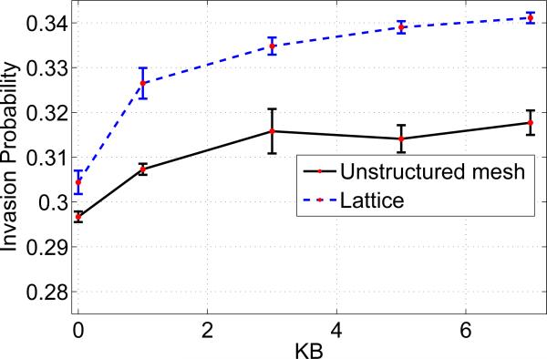
In order to compare with a 21×21 lattice that has 441 nodes, we designed an unstructured mesh consisting of 441 elements. However, to make a fair comparison with a lattice, we estimated the average number of neighbors for an unstructured mesh that has 441 elements. A set of sample realizations for an unstructured mesh was taken to obtain the average number of neighbors for an element, which was approximately 6. We took this number 6 as the nearest number of neighboring locations for each nodal point on a lattice on which a cell can give birth/migrate. The shape of the neighborhood of a node on the lattice is the von-Neumann neighborhood along with 2 diagonal nodes. Figure 6 displays a comparison of the invasion probabilities on an unstructured mesh and on a lattice with parameters λ = 1.5 and kA = 0. It is clearly evident that the lattice results overestimate the invasion probability. The difference in fixation probability grows with the migration parameter kB.
Figure 6.
Comparison of Invasion probabilities: Unstructured mesh (vs) Lattice. The average number of neighbors for the lattice are chosen to be approximately 6, i.e., the von-Neumann neighborhood along with diagonal nodes. Parameters: lattice size = 21 × 21, mesh size = 441 elements, λ = 1.5 and kA = 0.
For a high fitness advantage (λ = 1.5 ), the cluster expansion of mutants is increased, resulting in a non-significant effect of migration potentials on the invasion probability, i.e., the proliferation mechanism dominates the migration mechanism. Hence, we observe the migration potential to have a very minimal effect on the invasion probability for high fitness advantages.
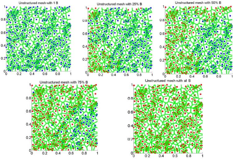
Figures (7)—(9) display the evolution and invasion of one type B cell to a saturated state containing all type B cells on an unstructured mesh. A blue color (dark in black and white) indicates normal or type A cells and a red color (light in black and white) denotes pre-cancerous or mutant cells (i.e. type B cells).
Figure 7.
Spatial evolution of B cell on an unstructured mesh.
3.3. Boundary effect on Lattice
We now consider the effects of the lattice boundary on the invasion probability. We investigate this by first constructing a 21 × 21 regular square grid. Instead of randomly placing a pre-cancerous cell on the grid, we fix its position on the boundary. Our system is now filled with 440 type A or host cells placed at every location and one type B cell placed on the boundary. The algorithm outlines in previous section is run using reflecting boundary conditions, and each iteration is performed until, for a fixed initial neighborhood, the system reaches fixation and we estimate the invasion probability.
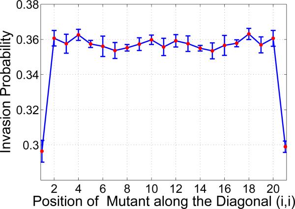
We investigate the variation in the invasion probability as a function of the initial location of type B cell, in particular, at the boundary. A lattice of 21 × 21 cells was constructed and the position of the type B cell was fixed at (i, i) = (1, 1), while the rest of the lattice was filled with type A cells. different sets of experiments were carried out by varying the initial position of the B cell along the diagonal, i.e. (i, i) = (2, 2), (3, 3), . . . , (11, 11), . . . , (21, 21). A sample scenario in which kA = 0 and λ = 1.5 is chosen for this purpose. We observe that the invasion probability is much smaller when compared to that at the center of the lattice. There is a sharp increase in the invasion probability when the initial position of the B cells is changed from (1, 1) to (2, 2), which remains constant as the initial position is moved to the center of the system (11, 11), and follows a similar pattern as observed in the previous case till it reaches (21, 21). Figure 10 displays the boundary effect for advantaged mutants and for various values of kB. Other scenarios with neutral and disadvantaged mutants, kA > 0, were also investigated and similar behavior of the system was observed. This clearly suggests that boundary effects have a predominant influence on the invasion probability. This is in agreement with the earlier, 1D results of [6].
4. Discussion
We have presented a computational approach to investigate an important but poorly understood phenomenon, phenotypic heterogeneity, which appears to be highly prevalent during various stages of tumor growth. The existence and adaptability of pre-cancerous cells with different fitness rates in human tissues is still far from an established fact. Thus, we formulated a simplified scenario and investigated mutant dynamics with only two pheno-types in our system under a confined tissue geometry. We have attempted to understand the effect of tissue geometry on the invasion probability by generating a random set of neighbors for each node on a regular grid. Also, we have focused on the use of unstructured meshes that we believe captures features of real tumors that structured meshes fail to do, and have analyzed the resulting invasion dynamics of mutants.
Random neighbors on a lattice
From Figure 1, we obtain some insight into the effects of the randomness of neighborhood sizes on the invasion probability in a migration free system. As noted previously, the invasion probability is negatively correlated with the width of the distribution of neighborhood size from Figures 1 and 2. An increase in the distribution width of the neighborhood size can completely eliminate the advantage given by an increased replication capacity of mutants, making them behave as if they were neutral. These results provide further justification for us to conjecture that tissue geometry plays an important role in the invasion dynamics of pre-cancerous cells within a confined region.
Invasion probability on unstructured mesh
The resulting graphs confirm that the invasion probability is much smaller on unstructured meshes compared to a regular grid. Interestingly, for the scenarios in which kA = 0 and kA = 1.0, and for a given λ = 1.5, we observe minimal effect on the invasion probability. This suggests that smaller migration potentials of the wild type has a smaller impact on the invasion probability. For a neutral mutant, we notice a significant change in the invasion probability for the scenarios kA = 0 and kA = 1.0. However, when the ratio of the replicative potentials is altered for various migration potentials, there is a huge impact on the invasion probability, which was observed from Figure 4. The effect on the trade-off between replicative and migrative potentials on the invasion probability is captured in Figure 4. Graphs (7)–(9) captures the morphology of mutant invasion for a sample realization. Our model is a generalized version of existing models and better captures the results on invasion dynamics.
Boundary effect on lattice
One of the results worth highlighting is the effect of the boundary on regular grids. This is done by fixing the position of a B cell in the system at (i, i) = (1, 1). This resulted in the invasion probability being smaller when compared to the invasion probability of a B cell placed at the center of the system. As the position of the B cell is moved inwards from the boundary, the invasion probability increases.
The models considered here are of course a simplification of reality on many levels. For example, experimental evidence suggests that more than one phenotype can co-exist during tumorigenesis [40]–[41], due to which the selection mechanism becomes very complicated. We do however ignore such complications in the present work.
We anticipate that our results can be used to better understand some mechanisms in tumor progression. This includes the effect of the tumor microenvironment, which can alter the proliferative and migrative potentials of cancer cells. Here, we used a simplified model to gain insights into the effect of invasion probability on random and unstructured meshes under two biological mechanisms, i.e. proliferation and migration. This model can be extended to include the randomness of fitness and migration potentials, as a result of heterogeneous tumor microenvironment and for distinct cell pheno-types. In addition, it is biologically known that the epithelial-mesenchymal transition (EMT) is a critical stage in metastasis, when cells acquire migrative capacity [42]. Our computational approach may be applied to address questions related to this biological phenomena. For example, we have shown that the invasion probability depends on the width of the distribution of neighbors. One might be able to experimentally validate this by inducing cells to undergo EMT and measuring the invasion probability for different tissue architectures (perhaps using different cell lines). In addition, we have observed that increasing migration potential (for example, due to EMT) has a significant effect if proliferative potential is around the neutral drift. Experimental studies of cells undergoing EMT in different microenvironment conditions (for instance, under normal and hypoxic conditions) might be used to validate this prediction. Finally, our results confirm that distortion of the tissue architecture and control of migration potential of pre-cancerous cells can reduce tumor progression to some degree. Also, the invasiveness of pre-cancerous cells can be controlled by a therapeutic agent that can inhibit alterations in the tissue geometry.
Figure 8.
Boundary effect on a Lattice: Invasion probability against the position of B mutant. Parameters: lattice size = 21 × 21, λ = 1.5 and kA = 0.
Acknowledgments
M. Kohandel and S. Sivaloganathan are supported by the Natural Sciences and Engineering Research Council of Canada (NSERC, discovery grants) as well as an NSERC/CIHR Collaborative Health Research grant. N. Komarova is supported by the NIH 1R01CA129286-01A1 grant.
Footnotes
Publisher's Disclaimer: This is a PDF file of an unedited manuscript that has been accepted for publication. As a service to our customers we are providing this early version of the manuscript. The manuscript will undergo copyediting, typesetting, and review of the resulting proof before it is published in its final citable form. Please note that during the production process errors may be discovered which could affect the content, and all legal disclaimers that apply to the journal pertain.
References
- 1.Nowell PC. The clonal evolution of tumor cell populations. Science. 1976;194:2328. doi: 10.1126/science.959840. [DOI] [PubMed] [Google Scholar]
- 2.Komarova NL, Sengupta A, Nowak MA. Mutation-selection networks of cancer initiation: tumor suppressor genes and chromosomal instability. J Theor Biol. 2003;223(4):433–450. doi: 10.1016/s0022-5193(03)00120-6. [DOI] [PubMed] [Google Scholar]
- 3.Nowak MA, Michor F, Komarova NL, Iwasa Y. Evolutionary dynamics of tumor suppressor gene inactivation. Proc. Natl Acad. Sci U.S.A. 2004;101(29):10635–10638. doi: 10.1073/pnas.0400747101. [DOI] [PMC free article] [PubMed] [Google Scholar]
- 4.Michor F, Iwasa Y, Rajagopalan H, Lengauer C, Nowak MA. Linear model of colon cancer initiation. Cell Cycle. 2004;3(3):358–362. [PubMed] [Google Scholar]
- 5.Iwasa Y, Michor F, Nowak MA. Stochastic tunnels in evolutionary dynamics. Genetics. 2004;166(3):1571–1579. doi: 10.1534/genetics.166.3.1571. [DOI] [PMC free article] [PubMed] [Google Scholar]
- 6.Komarova NL. Spatial stochastic models for cancer initiation and progression. Bull Math Biol. 2006;68(7):1573–1599. doi: 10.1007/s11538-005-9046-8. [DOI] [PubMed] [Google Scholar]
- 7.Komarova NL. Loss- and gain-of-function mutations in cancer: mass action, spatial and hierarchical models. J Stat Phys. 2007;128:413–446. [Google Scholar]
- 8.Thalhauser CJ, Lowengrub JS, Stupack D, Komarova NL. Selection in spatial stochastic models of cancer: Migration as a key modulator of fitness. Biol Direct. 2010;5:21. doi: 10.1186/1745-6150-5-21. [DOI] [PMC free article] [PubMed] [Google Scholar]
- 9.Foo J, Leder K, Michor F. Stochastic dynamics of cancer initiation. Phys Biol. 2011;8:015002. doi: 10.1088/1478-3975/8/1/015002. [DOI] [PMC free article] [PubMed] [Google Scholar]
- 10.Maruyama T. On the fixation probability of mutant genes in a subdivided population. Genet Res. 1970;15:221225. doi: 10.1017/s0016672300001543. [DOI] [PubMed] [Google Scholar]
- 11.Maruyama T. A markov process of gene frequency change in a geographically structured population. Genetics. 1974;76:367377. doi: 10.1093/genetics/76.2.367. [DOI] [PMC free article] [PubMed] [Google Scholar]
- 12.Maruyama T. A simple proof that certain quantities are independent of the geographical structure of population. Theor Popul Biol. 1974;5:148154. doi: 10.1016/0040-5809(74)90037-9. [DOI] [PubMed] [Google Scholar]
- 13.Slatkin T. Fixation Probabilities and Fixation Times in a Subdivided Population. Evolution. 1981;35(3):477–488. doi: 10.1111/j.1558-5646.1981.tb04911.x. [DOI] [PubMed] [Google Scholar]
- 14.Lieberman E, Hauert C, Nowak MA. Evolutionary dynamics on graphs. Nature. 2005;433:312–316. doi: 10.1038/nature03204. [DOI] [PubMed] [Google Scholar]
- 15.Houchmandzadeh B, Vallade M. The fixation probability of a beneficial mutation in a geographically structured population. New J. Physics. 2011;13:073020. [Google Scholar]
- 16.Deutsch A, Dormann S. Cellular automation modeling of biological pattern formation. Birkhauser; Boston: 2005. [Google Scholar]
- 17.Byrne H, Alarcn T, Owen M, Webb S, Maini P. Modeling Aspects of Cancer Dynamics: A Review. Phil. Trans. R. Soc. A. 2006;364:1563–1578. doi: 10.1098/rsta.2006.1786. [DOI] [PubMed] [Google Scholar]
- 18.Anderson A, Chaplain M, Rejniak K, Fozard J. Single-cell based models in biology and medicine. Math Med Biol. 2008;25:185–186. [Google Scholar]
- 19.Quaranta V, Rejniak K, Gerlee P, Anderson A. Invasion emerges from cancer cell adaptation to competitive microenvironments: Quantitative predictions from multiscale mathematical models. Sem Cancer Biol. 2008;18:338–348. doi: 10.1016/j.semcancer.2008.03.018. [DOI] [PMC free article] [PubMed] [Google Scholar]
- 20.Cristini V, Lowengrub J. Multiscale modeling of cancer: an integrated experimental and mathematical modeling approach. Cambridge University Press; 2010. [Google Scholar]
- 21.De Pillis L, Mallet D, Radunskaya A. Spatial tumor-immune modeling, Computational and Mathematical Methods in medicine. 2006;7(2-3):159–176. [Google Scholar]
- 22.Anderson A, Chaplain M. Continuous and discrete mathematical models of tumor-induced angiogenesis. Bulletin of mathematical biology. 1998;60(5):857–899. doi: 10.1006/bulm.1998.0042. [DOI] [PubMed] [Google Scholar]
- 23.Anderson A, Quaranta V. Integrative mathematical oncology. Nature Reviews Cancer. 2008;8(3):227–234. doi: 10.1038/nrc2329. [DOI] [PubMed] [Google Scholar]
- 24.Bartoszyński R, Edler L, Hanin L, Kopp-Schneider A, Pavlova L, Tsodikov A, Zorin A, Yakovlev AY. Modeling cancer detection: tumor size as a source of information on unobservable stages of carcinogenesis. Mathematical biosciences. 2001;171(2):113–142. doi: 10.1016/s0025-5564(01)00058-x. [DOI] [PubMed] [Google Scholar]
- 25.Bellomo N, Li N, Maini P. On the foundations of cancer modelling: selected topics, speculations, and perspectives. Mathematical Models and Methods in Applied Sciences. 2008;18(04):593–646. [Google Scholar]
- 26.Byrne H, Chaplain M. Growth of necrotic tumors in the presence and absence of inhibitors. Mathematical Biosciences. 1996;135(2):187–216. doi: 10.1016/0025-5564(96)00023-5. [DOI] [PubMed] [Google Scholar]
- 27.Chaplain M, McDougall S, Anderson A. Mathematical modeling of tumor-induced angiogenesis. Annu. Rev. Biomed. Eng. 2006;8:233–257. doi: 10.1146/annurev.bioeng.8.061505.095807. [DOI] [PubMed] [Google Scholar]
- 28.Enderling H, Anderson A, Chaplain M, Rowe G. Visualisation of the numerical solution of partial differential equation systems in three space dimensions and its importance for mathematical models in biology. Mathematical biosciences and engineering. 2006;3(4):571. doi: 10.3934/mbe.2006.3.571. [DOI] [PubMed] [Google Scholar]
- 29.Enderling H, Chaplain M, Anderson A, Vaidya J. A mathematical model of breast cancer development, local treatment and recurrence. Journal of theoretical biology. 2007;246(2):245–259. doi: 10.1016/j.jtbi.2006.12.010. [DOI] [PubMed] [Google Scholar]
- 30.Deisboeck T, Berens M, Kansal A, Torquato S, Stemmer-Rachamimov A, Chiocca E. Pattern of self-organization in tumour systems: complex growth dynamics in a novel brain tumour spheroid model. Cell Proliferation. 2008;34(2):115–134. doi: 10.1046/j.1365-2184.2001.00202.x. [DOI] [PMC free article] [PubMed] [Google Scholar]
- 31.Gaffney E. The application of mathematical modelling to aspects of adjuvant chemotherapy scheduling. Journal of mathematical biology. 2004;48(4):375–422. doi: 10.1007/s00285-003-0246-2. [DOI] [PubMed] [Google Scholar]
- 32.Gatenby R, Maini P. Mathematical oncology: cancer summed up. Nature. 2003;421(6921):321–321. doi: 10.1038/421321a. [DOI] [PubMed] [Google Scholar]
- 33.Gerlee P, Anderson A. An evolutionary hybrid cellular automaton model of solid tumour growth. Journal of theoretical biology. 2007;246(4):583–603. doi: 10.1016/j.jtbi.2007.01.027. [DOI] [PMC free article] [PubMed] [Google Scholar]
- 34.Hinow P, Rogers C, Barbieri C, Pietenpol J, Kenworthy A, DiBenedetto E. The dna binding activity of p53 displays reaction-diffusion kinetics. Biophysical journal. 2006;91(1):330–342. doi: 10.1529/biophysj.105.078303. [DOI] [PMC free article] [PubMed] [Google Scholar]
- 35.Lowengrub J, Frieboes H, Jin F, Chuang Y, Li X, Macklin P, Wise S, Cristini V. Nonlinear modelling of cancer: bridging the gap between cells and tumours. Nonlinearity. 2009;23(1):R1. doi: 10.1088/0951-7715/23/1/r01. [DOI] [PMC free article] [PubMed] [Google Scholar]
- 36.Macklin P, McDougall S, Anderson A, Chaplain M, Cristini V, Lowen-grub J. Multiscale modelling and nonlinear simulation of vascular tumour growth. J Theor Biol. 2009;58(4):765–798. doi: 10.1007/s00285-008-0216-9. [DOI] [PMC free article] [PubMed] [Google Scholar]
- 37.Moran P. The Statistical Processes of Evolutionary Theory Oxford: Clarendon. 1962 [Google Scholar]
- 38.Sood V, Antal T, Redner S. Voter Models on Heterogeneous Networks. Phys Rev E Stat Nonlin Soft Matter Phys. 77:2008. doi: 10.1103/PhysRevE.77.041121. [DOI] [PMC free article] [PubMed] [Google Scholar]
- 39.Josep Díaz Leslie Ann Goldberg, et al. Approximating Fixation Probabilities in the Generalized Moran Process. Algorithmica. 2012:1–14. [Google Scholar]
- 40.Tsao JL, Yatabe Y, Salovaara R, et al. Genetic reconstruction of individual colorectal tumor histories. Proc. Natl Acad. Sci., USA. 2000;97:12361241. doi: 10.1073/pnas.97.3.1236. [DOI] [PMC free article] [PubMed] [Google Scholar]
- 41.Tsao JL, Tavaré S, Salovaara R, et al. Colorectal adenoma and cancer divergence. Evidence of multilineage progression. Am. J. Pathol. 1999;154:18151824. doi: 10.1016/S0002-9440(10)65437-5. [DOI] [PMC free article] [PubMed] [Google Scholar]
- 42.Weinberg R. The biology of cancer. Garland Science Textbooks; 2006. [Google Scholar]


