Integrative Analysis of Many RNA-Seq Datasets to Study Alternative Splicing

Abstract

Alternative splicing is an important gene regulatory mechanism that dramatically increases the complexity of the proteome. However, how alternative splicing is regulated and how transcription and splicing are coordinated are still poorly understood, and functions of transcript isoforms have been studied only in a few limited cases. Nowadays, RNA-seq technology provides an exceptional opportunity to study alternative splicing on genome-wide scales and in an unbiased manner. With the rapid accumulation of data in public repositories, new challenges arise from the urgent need to effectively integrate many different RNA-seq datasets for study alterative splicing. This paper discusses a set of advanced computational methods that can integrate and analyze many RNA-seq datasets to systematically identify splicing modules, unravel the coupling of transcription and splicing, and predict the functions of splicing isoforms on a genome-wide scale.

1. Introduction

Alternative splicing is an important means of generating proteomic diversity. Recent estimates indicate that nearly 90% of human multi-exon genes are alternatively spliced [1]. The mechanisms regulating alternative splicing are still poorly understood, and their complexity attributes to the combinatorial regulation of many factors: e.g., splicing factors, cis-regulatory elements, and RNA secondary structures [2,3]. RNA-seq technology yields genome-wide, high-throughput expression profiles at many different levels of organization, and has opened up great opportunities for elucidating complex cellular activities at high resolution. From each RNA-seq dataset, we can derive not only the expression levels of genes, but also those of exons and transcripts (i.e., splicing isoforms). With such data, we can build three types of networks: (1) the exon co-splicing network, describing the relationships of how exons are co-spliced; (2) the transcript or isoform co-expression network; and (3) the gene co-expression network. Given many RNA-seq datasets, a collection of these three types of networks can be constructed to provide detailed information for deciphering alternative splicing at the exon, isoform, and gene levels.

However, the expression levels of exons, isoforms, and genes cannot be directly compared across RNA-seq studies with different platforms or from different labs, because systematic variations among datasets are often beyond the capability of statistical normalization. However, the correlations of expression profiles (or exon inclusion rate profiles) in different datasets are unitless and therefore comparable. As co-expression and co-splicing networks are constructed from such correlations, they are not affected by inter-dataset variations. Thus, modeling RNA-seq datasets as co-expression (co-splicing) networks provides an effective way to integrate a large number of RNA-seq experiments conducted in different laboratories, at different times, and using different technology platforms.

This paper reviews three studies with different biological viewpoints, which investigate genome-wide alternative splicing using state-of-the-art methods to integrate and analyze multiple networks derived from RNA-seq datasets. We begin by exploring exon co-splicing networks, to study how regulation is coordinated at the splicing level [4]. The next work discovers patterns in a series of two-layered coupled networks, in order to understand how transcriptional and splicing machinery are coupled and how they coordinate to regulate gene expression [5]. Finally, we perform the first systematic prediction of splicing isoform functions by integrating a set of isoform co-expression networks [6]. In each of the three studies, we propose an advanced computational method to model, integrate and analyze multiple networks at different genomic levels. We also provide either computational validation or supporting results from the literature to confirm the discovered patterns or novel function predictions.

2. Reconstruct splicing regulatory modules

A central concept in transcription regulation is the transcription module, defined as a set of genes that are co-regulated by the same transcription factor(s). Analogously, such coordinated regulation also occurs at the splicing level [7,8]. However, the study of coordinated splicing regulation has thus far been limited to individual cases [7,9,10]. In this paper, we define a splicing module as a set of exons that are regulated by the same splicing factors. The exons in a splicing module can belong to different genes, but they exhibit correlated splicing patterns (in terms of being included or excluded in their respective transcripts) across different conditions, thus forming an exon co-splicing cluster.

Given an RNA-seq dataset containing a set of samples, we calculate the inclusion rate of each exon¹ in every sample which is defined as the ratio between its expression level and that of the host gene. Using these rates, we can construct a weighted co-splicing network, where the nodes represent exons and the edge weights are the correlations between their inclusion rates, measured across all samples in the dataset. Furthermore, given a series of RNA-seq datasets, we can derive a series of co-splicing networks. The comparative analysis of these networks is an effective way to integrate a large number of RNA-seq experiments performed with different platforms and in different laboratories.

A heavy subgraph in a weighted co-splicing network represents a set of exons that are strongly correlated in their inclusion rate profiles; i.e., they are co-spliced. Exons that frequently form a heavy subgraph in multiple datasets are likely to be regulated by the same splicing factors, and thus form a splicing module. We call such patterns frequent co-splicing clusters (FSC). Frequent clusters are much less likely to be spurious patterns that heavy subgraphs identified in only a single network, and thus are more likely to represent real splicing modules. The FSC can be restated by the graph algorithm jargon as the “frequent dense vertexset (FDVS)” [11] or “recurrent heavy subgraph (RHS)” [12]. The only difference between the FDVS and RHS patterns is that they are defined based on the multiple unweighted networks and weighted networks, respectively. In [11], Yan et al. showed the advantage of identifying frequent clusters across multiple networks compared to identifying clusters in single networks or the summary network which is averaged across all individual networks. In [12], Li et al. further demonstrated the power and importance of weighted network analysis, compared with unweighted network pattern mining. In this work, we therefore adopted the tensor-based computational framework for effectively identifying FSCs from 38 weighted exon co-splicing networks derived from human RNA-seq datasets [4]. The method produced an atlas of FSCs, which we then validated against biological knowledge bases.

2.1. Problem Formulation

Our goal is to identify co-spliced exon clusters that frequently occur across multiple weighted co-splicing networks. A co-splicing network of n nodes (exons) can be represented as an n×n adjacency matrix A, where element a_ij is the weight of the edge between nodes i and j. This weight is the correlation between the two exons’ inclusion rate profiles. Given m co-splicing networks with the same n nodes but different edge weights, we can represent the whole system as a 3^rd-order tensor (or 3-dimensional array) A=(a_ijk)_n×n×m. An element a_ijk of the tensor is the weight of the edge between nodes i and j in the k^th network (Figure 1). A co-splicing cluster appears as a heavy subgraph in the co-splicing network, which in turn corresponds to a heavy region in the adjacency matrix. A frequent co-splicing cluster is one that appears in multiple datasets, and appears as a heavy subvolume of the tensor (Figure 1). Thus, the problem of identifying frequent co-splicing clusters can intuitively be formulated as the problem of identifying heavy subtensors in a tensor.

Figure 1.

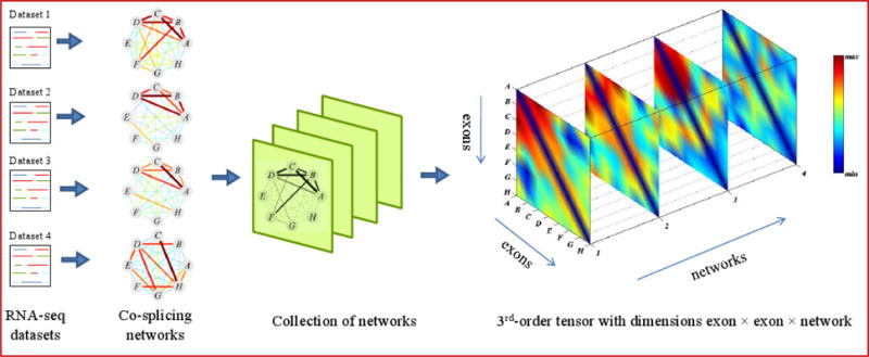
A collection of co-splicing networks can be stacked into a third-order tensor such that each slice represents the adjacency matrix of one network. The weights of edges in the co-splicing networks and their corresponding entries in the tensor are color-coded according to the scale to the right of the figure. After reordering the tensor by the exon and network membership vectors, a frequent co-splicing cluster (red) emerges in the top-left corner. It contains exons A, B, C, and D, which are heavily interconnected in networks 1, 2, and 3.

Representing a set of networks as a 3^rd-order tensor brings the following advantages: (1) the tensor model provides access to a wealth of numerical methods, in particular continuous optimization methods. In fact, reformulating discrete problems as continuous optimization problems is a long-standing tradition in graph theory. There are many successful examples, such as using a Hopfield neural network for the traveling salesman problem [13] and applying the Motzkin-Straus theorem to solve the clique-finding problem [14]. (2) Advanced continuous optimization techniques require very few ad hoc parameters, in contrast with heuristic graph algorithms. Both unweighted and weighted networks can be translated into tensor models treatable by the same tensor-based computational method. On the other hand, most existing graph methods applicable to unweighted networks cannot be easily adapted to weighted networks. (3) By transforming a graph pattern mining problem into a continuous optimization problem, it becomes easy to incorporate constraints representing prior knowledge.

A frequent co-splicing cluster in the tensor A can be defined by two membership vectors: (i) an exon membership vector x=(x₁,…,x_n)^T, where x_i=1 if exon i belongs to the cluster and x_i=0 otherwise; and (ii) a network membership vector y=(y₁,…,y_m)^T, where y_j=1 if the exons of the cluster are heavily interconnected in network j and y_j=0 otherwise. The summed weight of all edges in the FSC is

$$H_{\mathbf{A}}(x,y)=\frac{1}{2}{\displaystyle \sum }_{i=1}^n{\displaystyle \sum }_{j=1}^n{\displaystyle \sum }_{k=1}^m{a}_{\mathit{ijk}}{x}_i{x}_j{y}_k$$ (1)

Note that only the weights of edges a_ijk with x_i=x_j=y_k=1 are counted in H_A. Thus, H_A (x, y) measures the “heaviness” of the FSC defined by x and y. The problem of discovering a frequent co-splicing cluster can be formulated as a discrete combinatorial optimization problem: among all patterns of fixed size (K₁ member exons and K₂ member networks), find the heaviest. This is also an integer programming problem: find the binary membership vectors x and y that jointly maximize H_A under the constraints ${\sum }_{i=1}^n{x}_i=K_1$ and ${\sum }_{j=1}^n{y}_j=K_2$.

Although this discrete formulation is very intuitive, it has several major drawbacks to this discrete formulation. The first is parameter dependence, meaning that it is hard for users to suggest reasonable values for the size parameters K₁ and K₂. The second is high computational complexity; the optimization task is NP-hard, and therefore not solvable in a reasonable time even for small datasets. Therefore, the discrete formulation is infeasible for an analysis of many massive networks. However, we can solve a continuous optimization problem with the same objective by relaxing the integer constraints to continuous constraints. That is, we look for non-negative real vectors x and y that jointly maximize H_A. This problem is formally expressed as follows:

$$\begin{array}{l}\underset{x\in R_{+}^n,y\in R_{+}^n}{\max }{H}_{\mathbf{A}}(\mathit{x},\mathit{y})\\ \text{subject to}f(\mathit{x})=1\text{and}g(\mathit{y})=1\end{array}$$ (2)

where ${\mathrm{R}}_{+}^n$ is a non-negative real space, and f(x) and g(y) are vector norms. After solving Eq. (2), users can easily identify the top-ranking networks (after sorting the tensor by y) and top-ranking exons (after sorting each network by x) that contribute to the objective function. After rearranging the networks in this manner, the FSC with the largest heaviness occupies a corner of the 3D tensor. We can then mask all edges in the heaviest FSC with zeros and optimize Eq. (2) again to search for the next FSC.

The choice of vector norms in Eq. (2) has a significant impact on the outcome of the optimization. A vector norm defined as ${\Vert \mathit{x}\Vert }_p={({\sum }_{i=1}^n{\left|x_i\right|}^p)}^{1/p}$, p>0, is also called an “L_p-vector norm”. In general, the closer p is to zero, the sparser the solution favored by the L_p-norm. That is, the algorithm tends to find membership vectors where fewer components are significantly different from zero [15]. As p increases, the solutions favored by the L_p-norm grow smoother; in the extreme case p→∞, the elements of the optimized vector are approximately equal to each other. Our ideal membership vector is a compromise solution having a small number of exons (“sparse”) whose values are close to each other in magnitude (“smooth”), while the rest of exons are close to zero. Our past research [12] has shown that this goal can be achieved using the mixed norm L_0,∞(x) = α‖x‖₀ + (1 − α) ‖x‖_∞ (0 < α < 1) for f(x). The norm L₀ favors sparsity while the norm L_∞ encourages smoothness in the non-zero components of x. In practice, we approximate L_0,∞(x) with another mixed norm: L_p,2(x) = α‖x‖_p + (1 − α) ‖x‖₂ (0 < α < 1), where p<1. Our criterion for the network membership vector is that the exon cluster should appear in as many networks as possible, so the vector components should be non-zero and close to each other. This is the typical outcome of optimization using the L_∞ norm. In practice, we approximate L_∞ with L_q(y), where q>1 for g(y). Therefore, the vector norms f(x) and g(y) are fully specified as follows,

$$f(\mathit{x})=\alpha {\Vert \mathit{x}\Vert }_p+(1-\alpha ){\Vert \mathit{x}\Vert }_2\text{and}g(y)={\Vert \mathit{y}\Vert }_q$$ (3)

We performed simulations to determine suitable values for the parameters p, α, and q, applying our tensor method to collections of random weighted networks. We randomly placed FSCs of varying size, recurrence, and heaviness in a subset of the random networks. We then tried different combinations of p, α, and q, and adopted the combination (p=0.8, α=0.2, and q=10) that led to the discovery of the most FSCs.

2.2. Method

Since the vector norm f(x) is non-convex, our tensor method requires an optimization protocol that can deal with non-convex constraints. The quality of the optimum discovered for a non-convex problem depends heavily on the numerical procedure. Standard numerical techniques such as gradient descent converge to a local minimum of the solution space, and different techniques often just find different local minima. Thus, it is important to find a theoretically justified numerical procedure. We use an advanced framework known as multi-stage convex relaxation, which has good numerical properties for non-convex optimization problems [15]. In this framework, concave duality is used to construct a sequence of convex relaxations that give increasingly accurate approximations to the original non-convex problem. We approximate the sparse constraint function f(x) by the convex function ${\tilde{f}}_v(\mathit{x})={\mathit{v}}^{\mathrm{T}}h(\mathit{x})-f_h^{\ast }(\mathit{v})$, where h(x) is a specific convex function h(x)=x² and $f_h^{\ast }(\mathit{v})$ is the concave dual of the function ${\overline{f}}_h(\mathit{v})$ (defined as $f(\mathit{v})={\overline{f}}_h(h(\mathit{v}))$. The vector v contains coefficients that will be automatically generated during the optimization process. After each optimization, the new coefficient vector v yields a convex function ${\tilde{f}}_v(\mathit{x})$ that more closely approximates the original non-convex function f(x). For more details of our tensor-based optimization method, please refer to our original paper [12]. The source code is available on our website (http://zhoulab.usc.edu/tensor/).

Once the solution vectors of Eq. (2) have been found, frequent co-splicing clusters can be intuitively identified by including exons and networks with large membership values. However, a solution can result in multiple, overlapping patterns whose “heaviness” is greater than a specified threshold. Here, heaviness is defined as the average weight of all edges in a pattern. To identify the most representative pattern, we first rank exons and networks in decreasing order of their membership values in $\widehat{\mathit{x}}$ and $\widehat{\mathit{y}}$. Then we extract two representative patterns that satisfy the heaviness threshold: the pattern that occurs in the most networks while having a minimum number of top-ranking exons (this value is selected beforehand, for example 5), and the pattern with the largest number of top-ranking exons while appearing in a minimum number of top-ranking networks (e.g., 3). If these patterns are not the same, both are included as co-splicing clusters in our results. After discovering a pattern, we mask its edges in those networks where it occurs (replacing those elements of the tensor with zeroes) and optimize Eq.(2) again to search for the next most frequent co-splicing cluster.

2.3. Data sources

We identified 38 human RNA-seq datasets from the NCBI Sequence Read Archive, each with at least 6 samples providing transcriptome profiling under multiple experimental conditions, such as diverse tissues or various diseases. For each dataset, we used the Tophat [16] tool to map short reads to the hg19 reference genome, then applied the transcript assembly tool Cufflinks [17] to estimate expressions for all transcripts with known UCSC transcript annotations [18]. We calculated the inclusion rate of each exon as the ratio between its expression (the sum of FPKM² over all transcripts that cover the exon) and the host gene’s expression (the sum of FPKM over all transcripts of the gene). It is worth noting that in RNA-seq experiments, a gene expression with low FPKM is usually not precisely estimated, because the number of reads mapped to the gene is quite small. Therefore, in order to limit our analysis to reasonably accurate estimates, as pointed out by [19], we only calculated inclusion rates for those genes whose expressions are above 80th percentile in at least 6 samples. Applying this criterion resulted in inclusion rate profiles for 16,024 exons, covering 9,532 genes. We constructed an exon co-splicing network from each RNA-seq dataset, using Pearson’s correlation between the inclusion rate profiles across all samples as the edge weight between each exon pair. To make these correlation estimates comparable across datasets with different sample sizes, we applied Fisher’s z transform [20]. Given a PCC estimate r, Fisher’s transformation score was calculated as $z=0.5\ln (\frac{1+r}{1-r})$. The distributions of z-scores vary from dataset to dataset, so we standardized the z-scores to enforce zero mean and unit variance in each dataset [21,22]. By inverting the z-scores, the corresponding “normalized” correlations were obtained, and were used as edge weights in the networks. We then performed non-uniform edge sampling of these networks to speed up the computations. As FSC patterns predominately contain edges with large weights, this sampling method preferentially selects edges with large weights. Details of this sampling method refer to [12].

2.4. Results

We applied our method to 38 RNA-seq datasets generated under various experimental conditions, looking for FSCs with heaviness ≥ 0.4 and containing at least 5 exons. We identified 7,194/3,104/1,422/594 co-splicing clusters with recurrences ≥3/4/5/6, respectively. To assess the biological significance of the clusters, we evaluate the extent to which they represent functional modules and splicing modules.

Functional analysis

We evaluated the functional homogeneity of the host genes for each exon cluster using Gene Ontology (GO) annotations. To limit the search to specific functions, we filtered out GO terms associated with >300 genes. If the host genes of exons are statistically enriched in a GO term, with p-value<1E–4 (based on the hypergeometric test), then we declare the exon cluster to be functionally homogeneous. We found that 23.3% of the clusters appearing in ≥3 datasets are functionally homogenous, compared to 6.0% of randomly generated clusters with the same sizes. This ratio of 3.9 between the enrichment rates of clusters discovered in real data and random patterns is evidence that many of the discovered patterns have strong biological relevance. The enrichment ratio increases with the recurrence of FSCs, confirming the benefits of integrating multiple RNA-seq datasets to improve the quality of detected patterns. The functionally homogenous clusters cover a wide range of GO terms associated with post-transcriptional functions, such as “RNA splicing”, “ribonucleoprotein binding”, “heterogeneous nuclear ribonucleoprotein complex”, “negative regulation of transcription from RNA polymerase II promoter”, and “cellular protein localization”.

Splicing regulatory analysis

By construction, the exons in the discovered co-splicing clusters have highly correlated inclusion rate profiles across different experimental conditions. Such clusters are likely to consist of exons that are co-regulated by the same splicing factors. It has been shown that splicing factors can affect alternative splicing by interacting with cis-regulatory elements in a position-dependent manner [23]. We collected the experimental RNA target motifs (2220 RNA binding sites) of 62 splicing factors from the SpliceAid2 database [24]. To identify which splicing factors are associated with a co-splicing cluster, we performed the following analysis. First, for each exon of a co-splicing cluster, we retrieved the internal exon region and its 50bp flanking intron region which are enriched in the motifs of those 62 splicing factors by performing a BLAST search (E-score<0.001). If the exons of a cluster are highly enriched in the targets of a splicing factor, we consider the cluster to be “splicing homogeneous”. Although the collection of known splicing motifs is very limited, at the p-value<0.05 level (based on hypergeometric test), we still observed that 4.9% of the clusters with ≥5 exons and ≥6 recurrences are splicing homogenous, compared to 1.6% of randomly generated patterns with the same size distribution. The enrichment ratio is 3.0. Performing the same analysis for less frequent clusters, we found that the enrichment ratio decreases with the recurrence. The five most frequently enriched splicing factors are hnRNP E2, 9G8, hnRNP U, SRp75 and SRp30c. We also found that some splicing factors tend to co-bind to the cis-regulatory regions of exons in a co-splicing cluster, suggesting the combinatorial regulation of those splicing factors. We also found that combinatorial splicing regulation can occur in post-transcriptional processes.

3. Discovery of coupled transcription-splicing modules

In this research, we identify coupled transcription-splicing modules in a series of paired gene co-expression and exon co-splicing networks, where each pair of networks is derived from the same RNA dataset [5]. The concept of our approach is illustrated in Figure 2. A set of co-expressed genes (heavily interconnected in the gene co-expression networks) is likely to be co-regulated by the same transcription factor, and thus may represent a transcription module. Similarly, a set of co-spliced exons (heavily interconnected in the exon co-splicing networks) is likely to be co-regulated by the same splicing factor, and thus may represent a splicing module. When we find a transcription module wherein all or some of the exons form a splicing module, there is likely to implicate the transcription and splicing coupling is taking place. We call this a coupled module. Finally, if a coupled module (a co-expressed gene cluster coupled with a co-spliced exon cluster) appears in multiple gene-exon network pairs, then we call it a frequent coupled cluster (abbreviated FCC). Such clusters are much more likely to exemplify a real biological coupling mechanism than coupled modules found only in a single network pair.

Figure 2.

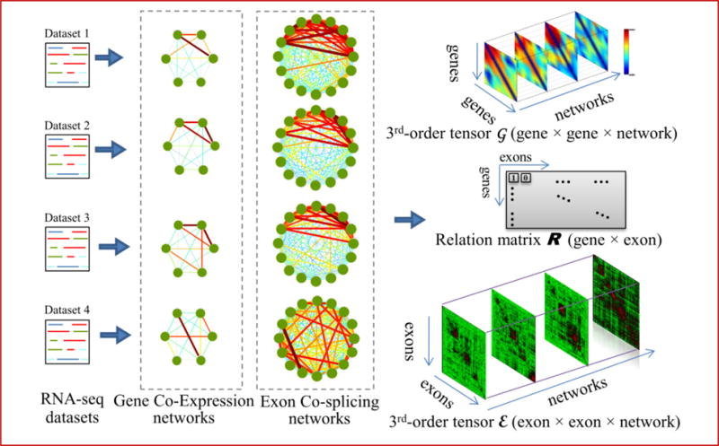
Illustration of the tensor model for collections of networks. From each RNA-seq dataset, we can build a gene co-expression network and an exon co-splicing network. Because all of the gene networks share the same set of genes, the collection of gene co-expression networks can be stacked into a third-order tensor G, such that each slice represents the adjacency matrix of one network. The same scenario applies to the exon co-splicing networks, which form a third-order tensor E. Weights of the edges in each network and their corresponding entries in the tensor are color-coded according to the scale at the right of the figure. The relationships between genes and exons in the two tensors are described by a binary matrix R, in which r_ij = 1 when the i^th gene contains the j^th exon; otherwise r_ij=0.

To identify FCCs in a large collection of edge-weighted co-expression and co-splicing network pairs, we propose another computational method based on the tensor model introduced in Section 2. Given L RNA-seq datasets, we can produce a collection of L gene co-expression networks with the same N gene nodes but different edge weights (correlations). This collection can be represented as a 3^rd-order tensor G=(g_ijk)_N×N×L (see Figure 2). Each element g_ijk is the weight of the edge between genes i and j, calculated from the k^th RNA-seq dataset. In the same way, a collection of L exon co-splicing networks with the same M exon nodes can be modeled as the tensor E=(e_ijk)_M×M×L. As each exon belongs to only one gene, but a gene may have more than one exon, we also need a relation matrix R with the following characteristics: (1) r_ij=1 when gene i contains exon j, r_ij=0 otherwise; and (2) each column vector has only one non-zero element. Therefore, R is very sparse, with exactly M non-zero elements.

As shown in Figure 3, an FCC can be described within the tensor model as follows. Its gene cluster and exon cluster intuitively correspond to heavy regions of the tensors G and E respectively. Thus, the FCC can be found by simultaneously reordering the tensors G and E such that the heaviest elements move toward the top-left corner, while their constituent genes and exons keep “belong-to” relationships. The heavy subvolume can then be expanded outwards from the left-top corner, until the FCC reaches its optimal size.

Figure 3.

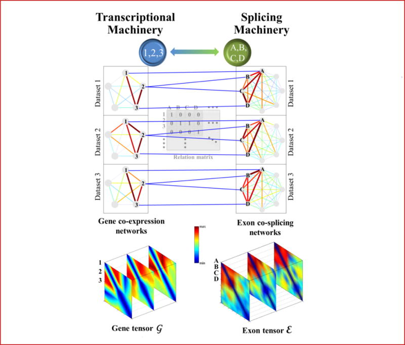
Illustration of a frequent coupled cluster (FCC). In a collection of three paired gene co-expression and exon co-splicing networks, a subset of genes {1,2,3} are heavily interconnected and their exons {A,B,C,D} are also heavily interconnected. These subsets form an FCC that represents the coupled transcription-splicing module. The gene and exon clusters intuitively correspond to the heavy subtensors in G and E.

3.1. Problem Formulation

In this section, we propose a novel computational method to identify FCCs. An FCC is defined as follows: “a set of genes G that are frequently co-expressed in a set of datasets D (forming a heavy subgraph in multiple gene networks), and a set of their exons E that are co-spliced in the same set of datasets (forming a heavy subgraph in multiple exon networks)”. Figure 3 gives an example. We formulate the problem of identifying an FCC as follows.

Definition of an FCC.

An FCC consists of a set of genes G, a set of exons E, and a set of datasets D that satisfy the following criteria:

Heavy Subgraph Criterion

Genes of G are heavily connected to each other in each dataset of D (these are called active datasets); exons of E are heavily connected to each other in the same set of datasets.

Relation Criterion

Each gene of G contains ≥1 exon of E, and each exon of E is contained by ≥1 gene of G.

An FCC can be described by three membership vectors: (i) the gene membership vector x = (x₁,…,x_N)^T, where x_i=1 if gene i belongs to the gene set G and x_i=0 otherwise; (ii) the exon membership vector y = (y₁,…,y_M)^T, where y_j=1 if exon j belongs to the exon set E and y_j=0 otherwise; and (iii) the dataset membership vector w = (w₁,…,w_L)^T where w_k=1 if the cluster appears (i.e., is sufficiently heavy) in the dataset k of D, and w_k=0 otherwise. We call the data sets in D “active datasets” for the cluster.

Using these three membership vectors, the “heavy subgraph criterion” can be formulated by maximizing the “heaviness” functions of the gene and exon subgraphs in the active datasets D. The “heaviness” function of a gene subgraph, $H_{\mathit{G}}(\mathit{x},\mathit{w})={\sum }_{i=1}^N{\sum }_{j=1}^N{\sum }_{k=1}^L{g}_{\mathit{ijk}}{x}_i{x}_j{w}_k$, is the summed weight of all edges of the subgraph in its active datasets. The “heaviness” function of an exon subgraph, $H_{\mathit{E}}(\mathit{y},\mathit{w})={\sum }_{i=1}^M{\sum }_{j=1}^M{\sum }_{k=1}^L{e}_{\mathit{ijk}}{y}_i{y}_j{w}_k$, is the summed weight of all edges of the subgraph in its active datasets D. Only the weights of edges between two member nodes (x_i=x_j=1, or y_i=y_j=1) are counted in H_G and H_E.

The “relation criterion” can be formulated by using the idea of the linear assignment problem formulation in operation science [25]. Let the relation variables Z=(z_ij)_N×M indicate the matching between genes and exons, where z_ij=1 if gene i contains exon j and both belong to the FCC, and 0 otherwise. Then the relation criterion can be implemented by maximizing the objective function $O_R(Z)={\sum }_{r_{\mathit{ij}}\ne 0}{z}_{\mathit{ij}}{r}_{\mathit{ij}}{x}_i{y}_j$ with the constraint ${\sum }_{j=1}^M{z}_{\mathit{ij}}\le K_2$ for all i=1,…,N, where K₂ is the number of exons in the cluster. Maximizing O_R(Z) can finds a set of genes and exons that are all related to each other, and simultaneously have large weights x_i and y_j in their respective membership vectors. This objective function suffices because the special characteristic of R already guarantees that each exon belongs to only one and only one gene.

Discovering an FCC can now be formulated as a discrete combinatorial optimization problem: among all FCCs of fixed size (K₁ member genes, K₂ member exons, and K₃ member datasets), we look for the pattern that maximizes the combined objective function O(x, y, w, Z) = H_G(x, w) + λH_E(y, w) + μO_R(x, y, Z), where λ, μ >0 are constant weights balancing the two criteria. This is an integer programming problem, which is not solvable in reasonable time even for small datasets. Instead we solve a continuous optimization problem with the same objective function, formally expressed as follows:

$$\begin{array}{l}\underset{x,y,w,Z\in R^{+}}{\max }O(\mathit{x},\mathit{y},\mathit{w},Z)=H_{\mathit{G}}(\mathit{x},\mathit{w})+\lambda H_{\mathit{E}}(\mathit{y},\mathit{w})+\mu O_R(\mathit{x},\mathit{y},Z)\\ \text{subject to}\{\begin{array}{ccc}\text{Constraint I:}& {\Vert \mathit{x}\Vert }_f=1,& 1\le f<2\\ \text{Constraint II:}& {\Vert \mathit{y}\Vert }_g=1,& 1\le g<2\\ \text{Constraint III:}& {\Vert \mathit{w}\Vert }_h=1,& h\ge 2\\ \text{Constraint IV:}& {{\displaystyle \sum }}_{j=1}^M{z}_{\mathit{ij}}\le 1,& i=1,2,\dots ,N\end{array}\end{array}$$ (4)

Constraints I and II above represent a well-known convex coding scheme [12,26] using the L_p=1 (1≤p<2) norm, which generates sparse solution vectors where only a few elements are significantly different from zero. Thus, the gene (exon) membership vector x(y) representing the module contains only a few genes (exons). On the other hand, the L_h=1 (h≥2) norm used in Constraint III generates a “smooth” solution vector whose elements are approximately equal; this leads to the discovered cluster occurring in as many datasets as possible.

Eq. (4) defines a tensor-based optimization framework for the problem of identifying FCCs. By solving Eq. (4), users can easily identify the top-ranking datasets (after sorting elements of w in non-increasing order) and top-ranking genes/exons (after sorting elements x/y in non-increasing order) contributing to the objective function. After rearranging the tensors in this manner, the optimum FCC occupies a corner of the 3D tensors G and E. We then mask the edges of this cluster in both networks with zeros, and optimize Eq. (4) again to search for the next module. The constant weights λ and μ in the objective function control the relative importance of the terms in the objective function. To fully exploit the power of this method, we collect all the FCCs discovered by our algorithm under several different combinations³ of λ and μ, then remove duplicates. The other three parameters, f, g and h, can be fixed through simulations.

3.2. Method

We derived an iterative algorithm to maximize the objective function with the constraints defined in Eq. (4). This algorithm repeatedly updates x, y, w, and Z, each time holding the other three variables fixed, until the objective function converges to a fixed point. The source code is available on our website (http://zhoulab.usc.edu/CMTensor/).

According to the definitions of the membership vectors x, y, and w, FCCs can be intuitively identified with the genes, exons, and datasets in the solution vectors that have the largest membership values. In this work, we empirically define an FCC extracted from the top-ranking genes, exons and datasets as a triplet (G′,E′,D′). We require an FCC to contain ≥5 genes G′, ≥5 exons E′ and ≥2 active datasets D′. Furthermore, we require that (1) each gene subgraph G′ and each exon subgraph E′ have an average edge weight (“heaviness”) >0.4; (2) at least 70% of the host genes of E′ are included in G′; and (3) at least 70% of all exons of the genes in G′ are included in E′. We refer to the ratios used in the second and third criteria as coverages: ${\mathit{\text{coverage}}}_{\text{gene}}(G\prime ,E\prime )=\frac{|G\prime \cap \mathit{\text{hostgene}}(E\prime )|}{|G\prime |}\ge 0.7$ and ${\mathit{\text{coverage}}}_{\text{exon}}(G\prime ,E\prime )=\frac{|E\prime \cap \mathit{\text{exon}}(G\prime )|}{|G\prime |}\ge 0.7$. The first criterion sets a standard for how heavy and frequent a cluster should be, while the second and third define the minimum degree of “coupling” between a gene set and an exon set.

We can often generate multiple overlapping FCCs from the set of top-ranking genes, exons, and datasets which satisfy all the criteria defined above. We refer to a group of overlapping FCCs derived from the same membership vectors x, y, and w as a family of FCCs.

3.3. Data sources

From the Sequence Read Archive of NCBI we selected all human RNA-seq datasets, each of which contains at least six samples (the minimum for robust correlation estimation). This results in a total of 38 datasets. For each dataset, we used the Tophat [16] tool to map short reads to the hg18 reference genome, then applied the transcript assembly tool Cufflinks [17] to estimate expressions for all transcripts with known UCSC annotations [18]. We calculated the inclusion rate of each exon in every sample, and the expression of its host gene. For each dataset, we built two networks: a weighted gene co-expression network, in which nodes represent genes and edges are weighted by expression correlations between two genes; and a weighted exon co-splicing network, in which nodes represent exons and edge weights represent correlations between the inclusion rates of two exons. We then performed the same network normalization procedure as introduced in Section 2.3, to make the edge weights comparable across datasets by removing the sample size effect. The normalized rates profile correlations were then used as edge weights in the networks We used non-uniform edge sampling when analyzing all networks to speed up the computations [12].

3.4. Results

After we applied our method to the 38 paired gene co-expression networks and exon co-splicing networks derived from RNA-seq datasets, we identified 8,667 FCC families containing a total of 43,580 FCCs. Each FCC contains ≥5 member genes, ≥5 member exons, and appears in ≥2 RNA-seq datasets; it also has heaviness ≥0.4, coverage_gene≥0.7, and coverage_exon≥0.7. The average number of genes/exons of these patterns is 12.61/12.64 and the average recurrence is 2.04. To assess the statistical significance of the FCCs, we also applied our method to 38 paired random networks, each of which is generated from one of the paired real networks by the edge randomization method⁴. We repeated this process 10 times, and each time only 0 ~ 3 FCC families (average 0.9 families) were identified. This is an extremely low value compared to the 8,667 FCC families discovered in real data.

3.4.1. Frequent coupled clusters are likely to represent transcription and splicing modules

Because the genes in an FCC are strongly co-expressed in multiple datasets generated under different conditions, they are likely to represent a transcription module. To assess this possibility, we used the 191 ChIP-seq profiles generated by the Encyclopedia of DNA Elements (ENCODE) consortium [27]. These data provide potential targets of regulatory factors that may or may not be active under a specific condition. However, if the gene set of an FCC is found to be highly enriched in the targets of a regulatory factor, then this factor is likely to actively regulate the genes in the FCC. Since FCCs within the same family are highly overlapping, we treat a family of FCCs as a unit in the following analyses. We denote a family of FCCs to be “transcriptionally homogenous” if any of its containing FCCs is significantly enriched in the targets of a regulatory factor. According to this definition, 61.2% of the identified FCC families are transcriptionally homogenous, with an enrichment q-value<0.05, compared to 8.9% of randomly generated patterns with the same size distribution. The five most frequently enriched regulators are YY1, E2F4, c-Myc, MAX, and TAF, all of which have been implicated in cancer pathogenesis or progression [28–32].

Since the exon set of an FCC has highly correlated inclusion rate profiles across different experimental conditions, they are likely to be co-regulated by the same splicing factors. We collected the experimental RNA target motifs (2,220 RNA binding sites) of 62 splicing factors from the SpliceAid2 database [24]. For each exon in an FCC, we retrieved the internal exon region and its 100bp flanking intron region which are enriched in the motifs of those 62 splicing proteins by performing a BLAST search (E-score <0.05). If the exon set of any FCC within a family is significantly enriched (q-value <0.05) in the targets of a splicing factor, we consider this family to be “splicing homogenous”. Although the collection of known splicing motifs is very limited, we still observed that 8.9% of the FCC families are splicing homogenous, compared to 5.1% of randomly generated patterns with the same size distribution. The five most frequently enriched splicing regulators are PSF, hnRNP-D, hnRNP-C1, SLM-2, and HuB.

3.4.2. Exploring the mechanisms of transcription and splicing coupling

In this section, we evaluate the hypothesis that the functionally coupled recruitment of transcription and splicing factors could be mediated by protein-protein interactions (PPIs), using data from the BioGRID repository [33]. We consider not only direct PPIs between two factors, but also indirect interactions through a mediator protein (i.e., one-hop interactions). Some experiments have shown that transcription and splicing factors can be recruited by the same other proteins [34,35]. In order to have a broad coverage, we used the 109 human transcription factors in the ENCODE [27] and JASPAR databases [36], and 10,278 DNA binding motifs downloaded from [37]. We performed a BLAST search (E-score <0.05) in 1000bp regions of the transcription start sites of all genes, and then used a hyper-geometric test (q-value <0.05) to identify transcription factors that are enriched among the genes of an FCC. The putative splicing factors for each FCC were identified as described in Section 3.4.1. The total number of PPIs between transcription and splicing factors within the same FCC families (including direct and one-hop interactions) is 105, compared to only 14.8 in random families with the same numbers of genes and exons. The enrichment ratio is 7.1, supporting the idea that PPI mediated association can be an important mechanism of transcription-splicing coupling.

4. Isoform function prediction with a multiple instance based label propagation method

Although recent years have seen an increase in the number of studies on isoform-specific functions, most functional annotations for proteins are still only recorded at the gene level. It remains unclear to what extent alternatively processed isoforms have divergent functions. To fill this gap, this section reports the first systematic prediction of isoform functions. We have designed a novel multiple instance based label propagation method that makes predictions by integrating many genome-wide RNA-seq datasets.

4.1. Problem and challenges

From an algorithmic viewpoint, the isoform function prediction problem is characterized by four major challenges:

1. The training data are unconventional. Most existing functional annotations are recorded for genes and not isoforms, yet each gene contains one or more isoforms. This type of data is called “multiple-instance (MI) labeled” data. In this framework, the isoforms are instances and each gene is a bag of isoforms. If a gene is labeled as having a function, then we know that at least one of its isoforms has this function; on the other hand, if a gene is labeled not to have the function, then none of its isoforms has this function.

2. The isoform function prediction task is unconventional. In fact, we want to make two types of predictions. The first is “inheritance prediction”: given a gene having a function, we want to know which of its isoform(s) “inherit” this function. The second is “de novo prediction”: we want to predict the functions of isoforms even for genes for which we have no information.

3. Integrating multiple isoform association networks with MI labels has never been done before. Many studies in the area of gene function prediction have implied that combining multiple data sources can result in higher-quality function predictions [38]. We believe that the same principle is valid for isoform function prediction. However, no method has been designed for the selection and integration of MI-labeled networks.

4. There is a dearth of validation data for isoform function prediction. To assess the performance of our predictions, we need functional annotations on some isoforms.

To address the first two challenges (i–ii), we propose a new technique called instance-oriented MI label propagation (abbreviated “iMILP”) that enables both inheritance and de novo predictions by exploiting the benefits of unlabeled data [6]. To address challenge (iii), we recast the network selection problem as a feature selection problem, and introduce a wrapper strategy to solve the problem. Figure 4 illustrates the iMILP and network selection and combination approaches. To address challenge (iv), we validate predictions using the set of isoforms whose host genes are annotated and contain only a single isoform.

Figure 4.

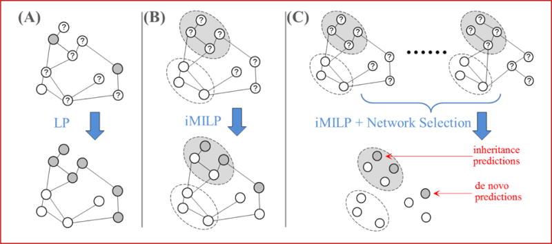
Illustrations of (A - LP) standard label propagation, with labels assigned to each node; (B - iMILP) the proposed instance-oriented MI label propagation, with labels assigned to bags of nodes; and (C - iMILP + Network Selection) the method of integrating multiple networks before iMILP. Each node represents an instance, and positive/negative/unknown nodes are drawn as gray/white/question-mark circles with solid lines. Positive/negative bags of instances are represented by the large gray/white ovals with dotted lines.

4.2. Methods

The proposed method consists of two components, as illustrated in Figure 5: (i) The network selection and combination component chooses the optimal subset of networks relevant to a given function among all input isoform co-expression networks, then aggregates them into a single network. This combined network is the input of the second component. (ii) The predictor component is a novel MI label propagation method. It returns function predictions for all isoforms by diffusing information from the labeled genes throughout the network of isoforms. These two components are explained in the following subsections.

Figure 5.

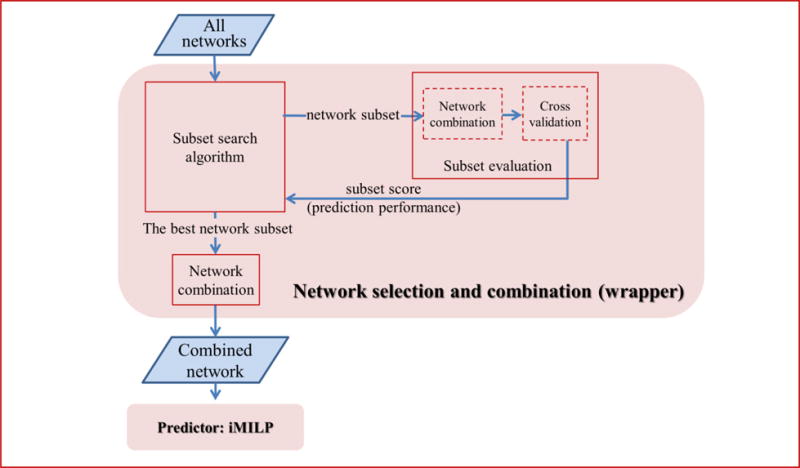
Flowchart of the proposed method with two components: “network selection and combination” and “predictor”. The network selection and combination step uses the wrapper feature selection strategy. The predictor component is our proposed iMILP method.

4.2.1. Instance-oriented MI label propagation method

All existing label propagation methods [39,40] for MI-labeled networks focus on classifying bags. They follow the rule that “knowing one of the instances in the bag is positive is sufficient for predicting this bag as positive”. However, an undesirable consequence of this rule is that in any positive bag, all but the single most positive instance are ignored. Therefore, these methods do not help when we need to answer a question such as “which instances are positive in the positive bag?” In our problem, we are more interested in knowing which isoforms (or instances) inherit the function of the gene (or bag) than which single isoform is the best representative of the function of the gene. We propose a novel instance-oriented MI label propagation (iMILP) method to make predictions at the instance level. Its label propagation rule is that “In the positive bag, a node (or instance) that links to more nodes from positive bags receives larger prediction scores; nodes that link to no other nodes from positive bags are demoted to have a prediction score of zero.” As we shall see, applying this rule iteratively to a well-chosen isoform network clearly identifies all instances that are qualified to inherit the bag’s label.

The isoform association network (with N isoforms) is represented as an adjacency matrix $W={\left(w_{\mathit{ij}}\right)}_{N\times N}$ where w_ij denotes the intensity of association (normalized Pearson’s correlation coefficient, PCC) between isoforms i and j. The normalized Laplacian of W is L = D^1/2WD^1/2, where D is a diagonal matrix with D_ii=Σ_jw_ij. For ease of presentation, we create a bag (called the “unlabeled bag”) to contain all the isoforms whose gene label is unknown (y=0). Unlike the positive and negative bags, the unlabeled bag does not correspond to a single gene. However, because none of the unlabeled genes and isoforms provides any constraints on the network, their isoforms can be grouped in this way without changing the result. Having defined the network and terminology, our proposed iMILP algorithm is as follows:

1. Initialize the soft label f of each node (isoform) in the positive, negative, or unlabeled bag (gene) as f=+1, −1 or 0, respectively.

2. Clamp the soft labels of nodes as follows:

   1. For nodes in the positive bags, f^new ← f when f> ε (ε is a positive number, close to zero), otherwise f^new ← 0.

   2. For nodes in the negative bags, f^new ← −1.

   3. For nodes in the unlabeled bag, the soft labels f remain unchanged: f^new ← f.

   4. For each bag (whether positive, negative, or unlabelled), normalize the scores f^new of all nodes in the bag, so that their squared sum is 1: f ← norm(f^new).

3. Diffuse labels: f ← Lf.

4. Repeat from Step 2 until f converges.

This algorithm adapts the pioneering label propagation approach [41] to the MI-labeled network. The diffusion step (3) propagates the information in the soft labels from the “source nodes” of labeled bags to neighbor nodes. Because the soft labels of source nodes are weakened by the diffusion step, the clamping step (2) restores their strength in the positive and negative bags, supporting the next round of the diffusion process. The clamping step should be performed on the bag level, so that the relative importance of nodes in a bag can be preserved.

In a positive bag, nodes with negative soft labels (or even more strictly, nodes with f<ε) are “demoted” to zero, as indicated in step 2(i). The threshold ε should be anti-correlated with the number of instances in the positive bag. In practice, we used $\epsilon =0.01/\sqrt{n}$. In a negative bag, following the MI labeling rule, all nodes must be negative and receive f scores equal to −1, as shown in step 2(ii). However, sometimes there are many negative bags, and the negative source nodes should not dominate the whole network. This problem is alleviated by the next step of normalizing f scores in the negative bags. The single “unlabeled bag” contains a large number of isoforms from different host genes. We keep their f scores unchanged, because these nodes serve as bridges for information to diffuse from the source nodes in labeled bags throughout the network. Nevertheless, we still normalize the unlabeled bag after each step, to guarantee that their soft labels converge. Therefore, the normalization step is important for all three types of bags, but has a slightly different purpose in each case.

Specifically, normalization in step 2(iv) means constraining the squared sum of the soft labels in a bag to 1. This step has three implications for the solution: (a) all bags are equal, (b) the soft label f of a node is always proportional to its contribution to the bag, and (c) the larger the bag, the lower the f scores of its nodes. Figure 6 illustrates the diffusion and clamping steps using an example network with 15 nodes. It can be observed that the f scores of the nodes inheriting labels in the positive/negative bags are replenished after each clamping step.

Figure 6. Illustration of the iMILP approach applied to a 15-node network.

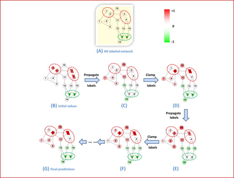
The initial network with its MI labels is shown in (A). Red dotted ovals represent positive bags of nodes, and green dotted ovals represent negative bags of nodes. (B) Each node is initialized according with soft labels according to step 1 of the iMILP algorithm. After a series of label propagation and clamping steps (C–F), the soft labels converge to network (G) which gives the final predictions. The shade of color in a node indicates the value of its soft label. The changing colors show that labels are propagated after each diffusion step, and that the soft labels in positive and negative bags are replenished after each clamping step, to prepare for the next diffusion step. In (G), both inheritance and de novo predictions are correctly made by the colors of the nodes.

After all the soft labels f converge, we need to make a final prediction for each node. For inheritance predictions, we assign positive labels to all nodes with non-zero f scores in the positive bags. The criterion should be more stringent for de novo predictions. We empirically set a threshold of 0.05, so that all nodes with f values at least this large in the unlabeled bag are predicted to be positive. The source code is available on our website (http://zhoulab.usc.edu/IsoFP).

4.2.2. Network selection and combination algorithm

In order to identify which isoform networks are the most informative for each function prediction, we recast the network selection problem as a feature selection problem. By viewing each network as a feature, we can take advantage of established feature selection strategies. The wrapper method is a widely used strategy [42]. As shown in Figure 5, it uses the prediction performance of a subset of networks to guide the search for the best subset. A prediction performance score is obtained by applying the predictive model to the current subset of networks, with ten random rounds of five-fold cross validation. The average AUC (area under the receiver operating characteristic curve) over all ten rounds is reported as the performance score. Our search algorithm employs a greedy sequential forward strategy [43] to find the best subset of networks. The “greedy” search heuristic adds a new network to the currently selected subset only if doing so improves the prediction performance. The detailed procedure is presented below. After selecting a subset of K networks G = {i₁,…,i_K}, we used equal weights to combine them into a single network: $\overline{W}={{\displaystyle \sum }}_{h\in G}{L}_h$, where L_h is the normalized Laplacian of network h.

4.3. Data sources

4.3.1. Isoform co-expression network construction

The mRNA isoform sequences were extracted from NCBI Reference Sequences (RefSeq) [44]. We discarded all RefSeq records that were not manually reviewed. To construct the isoform co-expression networks, we retrieved 29 datasets of human, full-length mRNA sequencing studies from the NCBI Sequence Read Archive database [45]. Each dataset was required to have at least 6 experiments, and not to be a population study. We used the eXpress [46] tool, combined with the Bowtie2 aligner [47], to infer isoform expression values. The RefSeq mRNA transcripts were used as transcriptome annotations. The mRNA level expression values were converted directly into protein isoform expressions. In cases where two or more RefSeq mRNA sequences correspond to the same protein sequence, they were regarded as belonging to a unique protein isoform, and their expression values were added.

In each RNA-seq dataset, a protein isoform was retained for further analysis only if the coefficient of variation (the ratio of standard deviation to mean) of its expression profile is ≥ 0.3 and significantly expressed with an expression value ≥10 FPKM in at least two experiments.

We calculated Pearson’s correlation coefficient (PCC) between the expression profiles of each isoform pair meeting the above criteria. We then performed the same network normalization procedure as introduced in Section 2.3 to obtain the normalized PCCs. For fast computation, only co-expressed isoform pairs with normalized PCCs ≥0.5 were included in the isoform co-expression networks.

4.3.2. Functional annotation of genes

Gene Ontology (GO) data [48] were used as function categories, and the UniProt Gene Ontology Annotation (UniProt-GOA) database [49] is our source of gene function annotations. Using the mapping information provided by the UniProt database, GO functions were assigned to each NCBI’s Gene ID, which includes one or more RefSeq transcripts. However, all GO annotations with the IEA (Inferred from Electronic Annotation) evidence code were removed from consideration in our analysis because they have not been verified by human curators. The GO terms are categorized into three major branches: Biological Process (BP), Cellular Component (CC) and Molecular Function (MF).

For a given GO term F, we labeled all its annotated genes as positive bags, and labeled those genes annotated with a sibling GO term as negative bags. The sibling GO terms of F are defined as those that share at least one direct parent with F and are not ancestors or descendants of F. We removed some functional categories from consideration using two criteria: (i) GO terms associated with >1000 genes (or <5 genes) were considered too general (or too specific). (ii) If a GO term has more than 95% of its associated genes also annotated with its sibling GO terms, it is considered indistinguishable from its siblings. After removing such terms, 4519 GO terms remained for use in our predictions and analysis.

4.4. Results

4.4.1. Prediction Performance of the iMILP method

The 29 RNA-seq datasets that we used to generate isoform co-expression networks cover a wide range of experimental and physiological conditions. We first applied our algorithm to each single network. However, no single network yielded an average AUC across all GO terms better than 0.53. The average AUC across all 29 single networks is only 0.48, worse than a random guess. Therefore, we applied the wrapper method to select and combine a different subset of networks for each GO term, based on their “usefulness” to the specific prediction at hand. The combined networks achieved dramatically better AUC scores, averaging to 0.67 across all GO terms. This result demonstrates the necessity of integrating multiple data sources for isoform function prediction.

4.4.2. Functional annotations of isoforms

Applying our method to the entire training dataset yielded 70,392 isoform-level function predictions. 13,621 of them were de novo predictions, meaning that the host genes are unannotated with respect to the predicted function in the current GO database. Therefore, as a side benefit, the iMILP method also contributes to function annotation at the gene level. In addition to the de novo results, we predicted the functions of 8,856 isoforms that have a least one annotation inherited from their host genes. In general, we believe that these inheritance predictions are more reliable than de novo predictions. Therefore, in the following analysis of the properties of isoform functions, we focused on inheritance predictions.

With the isoform-level annotations resolved, we were interested in seeing which gene functions are usually shared by many isoforms of the same gene, and which functions are only inherited by one or a small number of isoforms. We proposed the concept of inheritance rate (IR): given a GO term and a multi-isoform gene annotated by this term, IR is the ratio between the number of isoforms assigned to the GO term and the total number of isoforms for this gene. A high IR rate suggests that this function of the gene is robust against alternative isoform processing; otherwise the function is sensitive to this process. Among all GO terms annotated to at least 10 genes, the functions with the highest IR values are “nucleic acid transport”, “RNA splicing, via transesterification reactions”, “cellular protein localization” and “hair follicle maturation”. The functions that are most sensitive to the regulation of isoforms are “regulation of membrane potential”, “actin cytoskeleton reorganization”, “taxis” and “positive regulation of apoptotic process”.

4.4.3. Functional divergence among isoforms

Among the 7,714 multi-isoform genes annotated in the RefSeq database, 2,534 (791 or 1572) genes have at least two isoforms with functional predictions in the same GO branch (BP, CC or MF). For each of these genes, we calculated the functional dissimilarity averaged across all pairs of isoforms with annotations in the same GO branch. The similarity score of two isoforms was estimated using the G-SESAME method [50], and dissimilarity was simply defined as one minus the similarity score. The isoform functional divergence of a gene was calculated as the average dissimilarity score over all possible isoform pairs with GO annotations. Only isoforms that belong to the same gene and have predicted GO term(s) in the same GO tree branch were compared with each other to investigate functional dissimilarity.

We found that for all three GO branches, a large number of genes have isoforms that share the same or very similar functions (dissimilarity between 0 and 0.1). Specifically, among BP, CC and MF annotations, 19.0% (482), 44.8% (354) and 30.7% (483) of the genes respectively have multiple isoforms annotated with identical functions. Nevertheless, a small but significant proportion of genes have functionally distinct isoforms. For example, in the BP branch, 13.1% of genes have isoforms with a dissimilarity score greater than 0.5. The proportions for CC and MF terms are 4.9% and 5.2%, respectively.

5. Conclusion

Recent years have seen the rapid accumulation of RNA-seq data, which can measure cellular activities at high resolution. There is an increasing need for powerful computational tools capable of integrating many RNA-seq datasets to study splicing regulation. In this paper, we describe three novel computational approaches that can discover splicing modules and coupled transcription-splicing modules, and predict the functions of splicing isoforms. The first method is a network pattern mining algorithm by modelling a set of networks as a 3^rd-order tensor. It takes a set of exon co-splicing networks as input, and outputs clusters of exons which are densely interconnected in as many networks as possible. The analysis of the identified patterns demonstrated that the exon clusters with high recurrence are more likely to represent splicing modules than those occurring in only single networks. The second method is also a tensor-based pattern discovery algorithm for analyzing multiple coupled networks. It takes as input a large collection of coupled co-expression and co-splicing network pairs, and outputs patterns each of which consists of a co-expressed gene cluster coupled with a co-spliced exon cluster that frequently appears in multiple coupled networks. The identified coupling modules enable the exploration of how the transcription and splicing factors cooperate to regulate gene activities. Different from the first two methods which are unsupervised learning, the third method is essentially a semi-supervised learning approach. Taking as input a set of networks in which a small portion of nodes have multiple-instance class labels, this algorithm aims to classify those unlabeled nodes in the networks and outputs their predicted labels. This semi-supervised learning algorithm was applied to the isoform function prediction problem. The predicted isoform functions suggest that although many genes have isoforms carrying the same function, there is a substantial fraction of genes that are spliced into isoforms with diverse functions. These advanced computational approaches have provided effective analysis tools to integrate a large number of RNA-seq datasets for studying alternative splicing from various aspects. As more RNA-seq data are released to the public databases in the near future, such integrative analysis methods will grow in its ability to provide high-quality and high-resolution splicing patterns and functional annotations of the transcriptome.

References

- 1.Wang ET, Sandberg R, Luo S, Khrebtukova I, Zhang L, Mayr C, et al. Alternative isoform regulation in human tissue transcriptomes. Nature. 2008;456:470–476. doi: 10.1038/nature07509. [DOI] [PMC free article] [PubMed] [Google Scholar]
- 2.Matlin AJ, Clark F, Smith CWJ. Understanding alternative splicing: towards a cellular code. Nat Rev Mol Cell Biol. 2005;6:386–398. doi: 10.1038/nrm1645. [DOI] [PubMed] [Google Scholar]
- 3.Chen M, Manley JL. Mechanisms of alternative splicing regulation: insights from molecular and genomics approaches. Nat Rev Mol Cell Biol. 2009;10:741–754. doi: 10.1038/nrm2777. [DOI] [PMC free article] [PubMed] [Google Scholar]
- 4.Dai C, Li W, Liu J, Zhou XJ. Integrating many co-splicing networks to reconstruct splicing regulatory modules. BMC Syst Biol. 2012;6(Suppl 1):S17. doi: 10.1186/1752-0509-6-S1-S17. [DOI] [PMC free article] [PubMed] [Google Scholar]
- 5.Li W, Dai C, Liu CC, Zhou XJ. Algorithm to identify frequent coupled modules from two-layered network series: application to study transcription and splicing coupling. J Comput Biol. 2012;19:710–30. doi: 10.1089/cmb.2012.0025. [DOI] [PMC free article] [PubMed] [Google Scholar]
- 6.Li W, Kang S, Liu CC, Zhang S, Shi Y, Liu Y, et al. High-resolution functional annotation of human transcriptome: predicting isoform functions by a novel multiple instance based label propagation method. Nucleic Acid Res. doi: 10.1093/nar/gkt1362. In Press (n.d) [DOI] [PMC free article] [PubMed] [Google Scholar]
- 7.Ule A Jernej, Ule JS, Williams JSH Alan, Cline HW Melissa, Clark CF Tyson, Ruggiu BRZ Matteo, et al. Nova regulates brain-specific splicing to shape the synapse. Nat Genet. 2005;37:844–852. doi: 10.1038/ng1610. [DOI] [PubMed] [Google Scholar]
- 8.Hedley ML, Maniatis T. Sex-specific splicing and polyadenylation of dsx pre-mRNA requires a sequence that binds specifically to tra-2 protein in vitro. Cell. 1991;65:579–586. doi: 10.1016/0092-8674(91)90090-l. [DOI] [PubMed] [Google Scholar]
- 9.Moore MJ, Wang Q, Kennedy CJ, Silver PA. An Alternative Splicing Network Links Cell-Cycle Control to Apoptosis. Cell. 2010;142:625–636. doi: 10.1016/j.cell.2010.07.019. [DOI] [PMC free article] [PubMed] [Google Scholar]
- 10.Zhang C, Zhang Z, Castle J, Sun S, Johnson J, Krainer AR, et al. Defining the regulatory network of the tissue-specific splicing factors Fox-1 and Fox-2. Genes Dev. 2008;22:2550–2563. doi: 10.1101/gad.1703108. [DOI] [PMC free article] [PubMed] [Google Scholar]
- 11.Yan X, Mehan MR, Huang Y, Waterman MS, Yu PS, Zhou XJ. A graph-based approach to systematically reconstruct human transcriptional regulatory modules. Bioinformatics. 2007;23:i577–86. doi: 10.1093/bioinformatics/btm227. [DOI] [PubMed] [Google Scholar]
- 12.Li W, Liu CC, Zhang T, Li H, Waterman MS, Zhou XJ. Integrative analysis of many weighted co-expression networks using tensor computation. PLoS Comput Biol. 2011;7:e1001106. doi: 10.1371/journal.pcbi.1001106. [DOI] [PMC free article] [PubMed] [Google Scholar]
- 13.Hopfield JJ. Neural networks and physical systems with emergent collective computational abilities. Proc Natl Acad Sci USA. 1982;79:2554–2558. doi: 10.1073/pnas.79.8.2554. [DOI] [PMC free article] [PubMed] [Google Scholar]
- 14.Motzkin TS, Straus EG. Maxima for Graphs and a New Proof of a Theorem of Turán. Can J Math. 1965;17:533–540. [Google Scholar]
- 15.Zhang T. Analysis of Multi-stage Convex Relaxation for Sparse Regularization. J Mach Learn Res. 2010;11:1081–1107. [Google Scholar]
- 16.Trapnell C, Pachter L, Salzberg SL. TopHat: discovering splice junctions with RNA-Seq. Bioinformatics. 2009;25:1105–1111. doi: 10.1093/bioinformatics/btp120. [DOI] [PMC free article] [PubMed] [Google Scholar]
- 17.Trapnell C, Williams BA, Pertea G, Mortazavi A, Kwan G, van Baren MJ, et al. Transcript assembly and quantification by RNA-Seq reveals unannotated transcripts and isoform switching during cell differentiation. Nat Biotechnol. 2010;28:511–5. doi: 10.1038/nbt.1621. [DOI] [PMC free article] [PubMed] [Google Scholar]
- 18.Fujita PA, Rhead B, Zweig AS, Hinrichs AS, Karolchik D, Cline MS, et al. The UCSC Genome Browser database: update 2011. Nucleic Acids Res. 2011;39:D876–882. doi: 10.1093/nar/gkq963. [DOI] [PMC free article] [PubMed] [Google Scholar]
- 19.Jiang H, Wong WH. Statistical inferences for isoform expression in RNA-Seq. Bioinformatics. 2009;25:1026–1032. doi: 10.1093/bioinformatics/btp113. [DOI] [PMC free article] [PubMed] [Google Scholar]
- 20.Anderson TW. An introduction to multivariate statistical analysis. 3. Wiley-Interscience; Hoboken, NJ: 2003. [Google Scholar]
- 21.Xu M, Kao MCJ, Nunez-Iglesias J, Nevins JR, West M, Zhou XJ. An integrative approach to characterize disease-specific pathways and their coordination: a case study in cancer. BMC Genomics. 2008;9(Suppl 1):S12. doi: 10.1186/1471-2164-9-S1-S12. [DOI] [PMC free article] [PubMed] [Google Scholar]
- 22.Li W, Liu CC, Zhang T, Li H, Waterman MS, Zhou XJ. Integrative analysis of many weighted co-expression networks using tensor computation. PLoS Comput Biol. 2011;7:e1001106. doi: 10.1371/journal.pcbi.1001106. [DOI] [PMC free article] [PubMed] [Google Scholar]
- 23.Licatalosi DD, Mele A, Fak JJ, Ule J, Kayikci M, Chi SW, et al. HITS-CLIP yields genome-wide insights into brain alternative RNA processing. Nature. 2008;456:464–469. doi: 10.1038/nature07488. [DOI] [PMC free article] [PubMed] [Google Scholar]
- 24.Piva F, Giulietti M, Burini AB, Principato G. SpliceAid 2: A database of human splicing factors expression data and RNA target motifs. Hum Mutat. 2011 doi: 10.1002/humu.21609. [DOI] [PubMed] [Google Scholar]
- 25.Burkard R, Dell’Amico M, Martello S. Assignment Problems. SIAM. 2009 [Google Scholar]
- 26.Ding C, Zhang Y, Li T, Holbrook SR. Biclustering Protein Complex Interactions with a Biclique Finding Algorithm; Proc 6th Int Conf Data Min; Hong Kong, China. 2006. [Google Scholar]
- 27.Thomas DJ, Rosenbloom KR, Clawson H, Hinrichs AS, Trumbower H, Raney BJ, et al. The ENCODE Project at UC Santa Cruz. Nucleic Acids Res. 2007;35:D663–D667. doi: 10.1093/nar/gkl1017. [DOI] [PMC free article] [PubMed] [Google Scholar]
- 28.Gordon S, Akopyan G, Garban H, Bonavida B. Transcription factor YY1: structure, function, and therapeutic implications in cancer biology. Oncogene. 2005;25:1125–1142. doi: 10.1038/sj.onc.1209080. [DOI] [PubMed] [Google Scholar]
- 29.Nevins JR. The Rb/E2F pathway and cancer. Hum Mol Genet. 2001;10:699. doi: 10.1093/hmg/10.7.699. [DOI] [PubMed] [Google Scholar]
- 30.Little CD, Nau MM, Carney DN, Gazdar AF, Minna JD. Amplification and expression of the c-myc oncogene in human lung cancer cell lines. 1983 doi: 10.1038/306194a0. [DOI] [PubMed] [Google Scholar]
- 31.Nair SK, Burley SK. X-Ray Structures of Myc-Max and Mad-Max Recognizing {DNA}: Molecular Bases of Regulation by Proto-Oncogenic Transcription Factors. Cell. 2003;112:193–205. doi: 10.1016/s0092-8674(02)01284-9. [DOI] [PubMed] [Google Scholar]
- 32.Suzuki H, Igarashi S, Nojima M, Maruyama R, Yamamoto E, Kai M, et al. IGFBP7 is a p53-responsive gene specifically silenced in colorectal cancer with CpG island methylator phenotype. Carcinogenesis. 2010;31:342. doi: 10.1093/carcin/bgp179. [DOI] [PubMed] [Google Scholar]
- 33.Stark C, Breitkreutz BJ, Reguly T, Boucher L, Breitkreutz A, Tyers M. BioGRID: a general repository for interaction datasets. Nucleic Acids Res. 2006;34:D535. doi: 10.1093/nar/gkj109. [DOI] [PMC free article] [PubMed] [Google Scholar]
- 34.Nayler O, Strätling W, Bourquin JP, Stagljar I, Lindemann L, Jasper H, et al. SAF-B protein couples transcription and pre-mRNA splicing to SAR/MAR elements. Nucleic Acids Res. 1998;26:3542. doi: 10.1093/nar/26.15.3542. [DOI] [PMC free article] [PubMed] [Google Scholar]
- 35.Blencowe BJ, Bowman JAL, McCracken S, Rosonina E. SR-related proteins and the processing of messenger RNA precursors. Biochem Cell Biol. 1999;77:277–291. [PubMed] [Google Scholar]
- 36.Sandelin A, Alkema W, Engström P, Wasserman WW, Lenhard B. JASPAR: an open-access database for eukaryotic transcription factor binding profiles. Nucleic Acids Res. 2004;32:D91–94. doi: 10.1093/nar/gkh012. [DOI] [PMC free article] [PubMed] [Google Scholar]
- 37.Tabach Y, Brosh R, Buganim Y, Reiner A, Zuk O, Yitzhaky A, et al. Wide-scale analysis of human functional transcription factor binding reveals a strong bias towards the transcription start site. {PloS} One. 2007;2:e807. doi: 10.1371/journal.pone.0000807. [DOI] [PMC free article] [PubMed] [Google Scholar]
- 38.Noble W, Ben-Hur A. Bioinformatics-From Genomes to Ther. 2007. Integrating information for protein function prediction; pp. 1297–1314. [Google Scholar]
- 39.Jia Y, Zhang C. Proc 23rd Natl Conf Artif Intell. AAAI Press; 2008. Instance-level semisupervised multiple instance learning; pp. 640–645. [Google Scholar]
- 40.Wang C, Zhang L, Zhang HJ. Graph-based multiple-instance learning for object-based image retrieval; Proceeding 1st ACM Int Conf Multimed Inf Retr – MIR ’08; New York, New York, USA. ACM Press; 2008. pp. 156–163. [Google Scholar]
- 41.Zhu X, Ghahramani Z. Learning from labeled and unlabeled data with label propagation. 2002. [Google Scholar]
- 42.Saeys Y, Inza I, Larrañaga P. A review of feature selection techniques in bioinformatics. Bioinformatics. 2007;23:2507–17. doi: 10.1093/bioinformatics/btm344. [DOI] [PubMed] [Google Scholar]
- 43.A model-free greedy gene selection for microarray sample class prediction. (n.d.) [Google Scholar]
- 44.Pruitt KD, Tatusova T, Brown GR, Maglott DR. NCBI Reference Sequences (RefSeq): current status, new features and genome annotation policy. Nucleic Acids Res. 2012;40:D130–5. doi: 10.1093/nar/gkr1079. [DOI] [PMC free article] [PubMed] [Google Scholar]
- 45.Leinonen R, Sugawara H, Shumway M. The sequence read archive. Nucleic Acids Res. 2011;39:D19–21. doi: 10.1093/nar/gkq1019. [DOI] [PMC free article] [PubMed] [Google Scholar]
- 46.Roberts A, Pachter L. Streaming fragment assignment for real-time analysis of sequencing experiments. Nat Methods. 2013;10:71–3. doi: 10.1038/nmeth.2251. [DOI] [PMC free article] [PubMed] [Google Scholar]
- 47.Liu Y, Schmidt B. Long read alignment based on maximal exact match seeds. Bioinformatics. 2012;28:i318–i324. doi: 10.1093/bioinformatics/bts414. [DOI] [PMC free article] [PubMed] [Google Scholar]
- 48.Ashburner M, Ball CA, Blake JA, Botstein D, Butler H, Cherry JM, et al. Gene ontology: tool for the unification of biology. The Gene Ontology Consortium. Nat Genet. 2000;25:25–9. doi: 10.1038/75556. [DOI] [PMC free article] [PubMed] [Google Scholar]
- 49.Barrell D, Dimmer E, Huntley RP, Binns D, O’Donovan C, Apweiler R. The GOA database in 2009–an integrated Gene Ontology Annotation resource. Nucleic Acids Res. 2009;37:D396–403. doi: 10.1093/nar/gkn803. [DOI] [PMC free article] [PubMed] [Google Scholar]
- 50.Wang JZ, Du Z, Payattakool R, Yu PS, Chen CF. A new method to measure the semantic similarity of GO terms. Bioinformatics. 2007;23:1274–81. doi: 10.1093/bioinformatics/btm087. [DOI] [PubMed] [Google Scholar]
- 51.Maslov S, Sneppen K. Specificity and Stability in Topology of Protein Networks. Science (80-) 2002;296:910–913. doi: 10.1126/science.1065103. [DOI] [PubMed] [Google Scholar]