Spatial scale and place field stability in a grid-to-place cell model of the dorsoventral axis of the hippocampus

Abstract

The rodent hippocampus and entorhinal cortex contain spatially-modulated cells that serve as the basis for spatial coding. Both medial entorhinal grid cells and hippocampal place cells have been shown to encode spatial information across multiple spatial scales that increase along the dorsoventral axis of these structures. Place cells near the dorsal pole possess small, stable, and spatially selective firing fields, while ventral cells have larger, less stable and less spatially selective firing fields. One possible explanation for these dorsoventral changes in place field properties is that they arise as a result of similar dorsoventral differences in the properties of the grid cell inputs to place cells. Here we test the alternative hypothesis that dorsoventral place field differences are due to higher amounts of non-spatial inputs to ventral hippocampal cells. We use a computational model of the entorhinal-hippocampal network to assess the relative contributions of grid scale and non-spatial inputs in determining place field size and stability. In addition, we assess the consequences of grid node firing rate heterogeneity on place field stability. Our results suggest that dorsoventral differences in place cell properties can be better explained by changes in the amount of non-spatial inputs, rather than by changes in the scale of grid cell inputs, and that grid node heterogeneity may have important functional consequences. The observed gradient in field size may reflect a shift from processing primarily spatial information in the dorsal hippocampus to processing more non-spatial, contextual and emotional information near the ventral hippocampus.

Introduction

So called “grid cells” in the medial entorhinal cortex (mEC), and “place cells” in the hippocampus are thought to play critical roles in rodent spatial navigation, and have been the subject of a large number of experimental and theoretical investigations aimed at understanding the neural underpinnings of spatial representation. Both cell types display firing patterns that correlate with an animal’s location in space. Place cells fire when an animal traverses a particular region of space, which is referred to as that cell’s “place field” (O’Keefe, 1976). Grid cells also fire with respect to particular locations, however, instead of firing at a single location, grid cells fire in a triangular “grid” lattice of locations (“grid nodes”) that extends throughout space (Hafting et al., 2005).

Experiments have shown that both the spatially-periodic firing fields of grid cells and the spatially localized firing fields of place cells show systematic increases in spatial scale along the dorsoventral axes of the mEC and hippocampus, respectively (Brun et al., 2008, Kjelstrup et al., 2008), which has led to the speculation that place field size is determined primarily by the spatial scale of a place cell’s grid cell inputs (McNaughton et al., 2006; Moser et al., 2008; Solstad et al., 2006). However, in addition to receiving spatially-modulated entorhinal inputs, ventral place cells also receive considerable amounts of non-spatial inputs from sources such as the amygdala and the hypothalamus (Witter et al., 1989, Risold and Swanson, 1996, Petrovich et al., 2001) or from neuromodulatory centers such as the ventral tegmental area (Gasbarri et al., 1997), which may also be important in determining place cell firing properties and could play a role in producing dorsoventral place field differences. This suggests an alternative hypothesis for why ventral place fields are larger than dorsal fields, namely that ventral cells increasingly process other, non-spatial types of information. The dorsoventral gradient in field size would then indicate a gradient of spatial information processing rather than reflecting the gradient of grid scales in the mEC. This view is supported by previous anatomical, behavioral, and gene expression studies suggesting functional distinctions between the dorsal and ventral hippocampal regions (Moser and Moser, 1998, Kjelstrup et al., 2002, Steffenach et al., 2005, Czerniawski et al., 2009).

Here we study a computational feed-forward network model of the entorhinal-hippocampal projections incorporating both a modular organization of grid cell inputs arranged in order of increasing spatial scale, as seen experimentally in the mEC (Brun et al., 2008; Hafting et al., 2005; Stensola et al., 2012), as well as a dorsoventral gradient of non-spatial inputs to place cells. In our model, as in a number of previous studies, place fields are formed via “winner-take-all” competition among place cells (de Almeida et al., 2009a; de Almeida et al., 2009b; Monaco and Abbott, 2011). Using this model, we test the hypothesis that dorsoventral differences in place cell activity result from corresponding differences in the amount of non-spatial inputs, rather than from the spatial scale of their grid cell inputs. Additionally, we assess the effects of grid node firing rate variability on place field stability.

Methods

Our model extends that of de Almeida et al (de Almeida et al., 2009a). We develop a rate-based model in which place cells are driven by excitatory inputs from the mEC and other areas. Mutual competition among place cells ensures that only a fraction of place cells will be active at any location, leading to spatial specificity as we explain below.

Inputs into place cells

Grid cells

The spatially periodic firing patterns of grid cells are modeled using the functions:

$$G(r,\lambda ,\theta ,c)=g(\sum _{k=1}^{3}cos(\frac{4\pi }{\sqrt{3}\lambda }\stackrel{\rightharpoonup }{u}({\theta }_k+\theta )·(\stackrel{\rightharpoonup }{r}-\stackrel{\rightharpoonup }{c})))$$ (1)

Here r = (x,y) is the location of the animal in space, λ is the inter-vertex spacing between grid points (in cm), c = (x₀,y₀) is the spatial phase (in cm relative to the origin), θ is the grid orientation, and u(θ_k) = (cos(θ_k),sin(θ_k)) is the unit vector in the direction θ_k.. Here θ₁ = −π/6, θ₂ = π/6, and θ₃ = π/2. The grid pattern is formed by summing three planar sinusoids with three different orientations, and then passing the result through a function g(x), given by g(x) = exp[a(x –b)]−1, where a = 0.3 and b = −3/2 are shape parameters chosen to match experimental data (de Almeida et al., 2009a). The function G(r,λ,θ,c) defines the activity level of a grid cell at a point r in space given parameters λ, θ, and c. Finally, we normalize the grid field firing rates by dividing by the peak firing rate, such that all of the grid nodes have peak firing rates equal to 1 prior to the introduction of firing rate variability in the grid nodes (see below). Here we interpret 1 as being equivalent to the peak firing rate of a typical grid cell, which is generally on the order of 10–15 Hz (Hafting et al., 2005).

For practical and technical reasons, most experiments on grid and place cells have been conducted in small enclosures (1m² scale). However, recent work (Brun et al., 2008; Kjelstrup et al., 2008) has shown that spatial representations may involve much larger scales, and in large environments are likely to involve more ventral levels of the hippocampal formation. Consequently, throughout this work, we run our simulations in two conditions of maximum grid scales of 1m² and 3.5 m².

Grid node firing rate variability

In most simulations we vary the firing rate of different nodes of a given grid cell in order to introduce firing rate heterogeneity similar to what is observed in experimental data. To do so, we keep the locations of the individual grid node fixed and scale the amplitude of each grid node independently by a random amount sampled from a truncated Gaussian distribution with mean 1 and standard deviation given by a parameter ξ. Thus the amount of grid node variance is controlled by ξ.

Non-Spatial inputs

In addition to receiving inputs from grid cells, place cells receive excitatory inputs from a pool of “non-spatial,” cells. Non-spatial cells are modeled as tonically-firing cells with firing rates that do not change as a function of space. Since relatively little is known about the physiology of non-spatial inputs into place cells, we assign the non-spatial cells in our model firing rates randomly drawn between 0 and a maximum value NS_max.

Network architecture and competitive mechanisms

Modular organization and grid cell to place cell connectivity

Recent experimental evidence supports the hypothesis that grid cells are functionally and anatomically segregated into distinct discrete modules at different points along the dorsoventral axis of the mEC (Stensola et al., 2012). In addition, a recent theoretical study of the relationship between grid cells and place cells found that place cell remapping is more complete when grid cells are organized into independently remapping modules (Monaco and Abbott, 2011). In an attempt to reproduce and investigate changes in place field properties along the dorsoventral axis of the hippocampus, we introduce a modular organization into the populations of grid cells and discretize the dorsoventral axis of the hippocampus by dividing the place cell population into 50 sub-populations, each at a different dorsoventral level. Model results were not sensitive to the specific number of sub-populations - whereas the number 50 was chosen in order to provide a reasonably fine discretization while still remaining computationally tractable, we experimented with values ranging from 25–100. We also restrict the connections between grid and place cells such that place cells in a particular portion of the dorsoventral axis receive the majority of their input from grid cells at the same dorsoventral level.

Figure 1 displays a diagram of the structure of the model. There are ten grid cell modules each containing 3000 grid cells, such that each grid module contains cells with fixed grid spacing (λ = 30,60,100 in Fig 1). The orientations of the grids within each module are similar to within 10 degrees of one another. These modules are arranged in order of their grid spacing in such a way as to mimic the experimentally observed increase in grid scale along the dorsoventral axis of the mEC (Brun et al., 2008; Stensola et al., 2012).

Figure 1. Diagram of the model.

In the model, grid cells are organized into 10 discrete modules, and the place cell population is discretized into 50 sub-populations. Grid cells within a particular module have a common spatial frequency and similar orientation (within 10 degrees) but random phase. The scale of the grids increases systematically from the first (Dorsal) module to the last (Ventral) module. Place cells in a given dorsoventral level receive the bulk of their inputs from the grid module at the same dorsoventral level, however some fraction of their inputs can also come from nearby grid modules. Place cells also receive some fraction of their total excitatory input from a pool of non-spatial cells.

Place cell populations

The collection of place cells is discretized dorsoventrally into 50 groups with 2000 place cells each. Here each group is a collection of place cells assumed to have the same connectivity statistics with respect to their inputs. Furthermore, cells at the same dorsoventral level are assumed to mutually interact to form their individual place fields via the E%-max winner-take-all mechanism described below. Throughout the paper we refer to place cell groups as being either “dorsal” or “ventral” as a function of the dorsoventral position of their corresponding primary grid cell input module.

In organizing our place cells into discrete groups, we make the implicit assumption that the inhibitory interactions involved in the winner-take-all competition are confined to a local portion of the dorsoventral axis of the hippocampus. This is an idealization of the assumption that winner take-all-competition does not take place across the entire dorsoventral axis of the hippocampus, but only locally, across (possibly overlapping) subpopulations. We can adjust the degree of overlap in the winner-take-all interactions between neighboring place cell groups but for the bulk of our simulations we assume that it is small (only 10% of the cells participating in the winner-take all competition come from neighboring place cell groups). For a more detailed discussion on the effect of overlap in the winner-take-all competition along the dorsoventral axis, see Figure 6 and the associated text in the Results.

Figure 6. Effect of overlap between place cell modules in the winner-take all interactions.

Plots of the proportion of active cells at different dorsoventral locations, for four different amounts of overlap in the winner-take-all interactions between neighboring groups of place cells, with a gradient in non-spatial inputs corresponding to β=0.85. As the amount of overlap in the winner-take-all interactions increases, there is an increasing tendency for more ventral cells (which receive more excitation in the form of non-spatial inputs) to suppress the activity of dorsal cells. Therefore, in order to produce realistic numbers of active dorsal cells, the amount of overlap must be low, implying that the winner-take-all inhibition governing place field formation should be confined to local regions of the dorsoventral axis.

The winner-take-all mechanism of place field formation

Our model of the place cell ensemble is inspired by that of de Almeida et al. (de Almeida et al., 2009a; de Almeida et al., 2010; Renno-Costa et al., 2010). In the model, hippocampal place fields result from the summed excitatory input from a random subset of grid cells, coupled with a competitive interaction between place cells referred to as the “E%-max winner-take-all” rule (de Almeida et al., 2009a; de Almeida et al., 2009b). In contrast to other proposals (Fuhs and Touretzky, 2006; Hayman and Jeffery, 2008; McNaughton et al., 2006; Si and Treves, 2009; Solstad et al., 2006), this class of models does not require any type of learning mechanism, or that place cells receive inputs from grid cells with a common spatial phase in order to produce well-defined place fields. We do not include any form of synaptic plasticity or learning in this model, despite the potential role of long term plasticity in refining and stabilizing place fields over the course of longer-term exposure to an environment. Other models for place field formation exist, which involve a linear summation of grid fields followed by the application of a spatially-uniform inhibition (Solstad et al., 2006). However, we choose to use a winner-take-all model with spatially varying inhibition for several reasons: 1) Summation models require precise and stable synaptic tuning of the connections between grid cells and place cells, 2) Such models do not directly explain why some cells have place fields and others do not in a given environment, and 3) Summation models make no natural predictions with respect to the sparsity of activity in the population of place cells.

The first step in computing the place fields for a given place cell is to compute the excitatory input to that cell at each point in space. This excitatory input at a particular location r is given by:

$$I_{i,m}(r)=\sum _{j=1}^{N_{\mathit{grid}}}{W}_{ij}{G}_j(r)+\sum _{k=1}^{N_{\mathit{nonspat},m}}{W^{\prime }}_{ik}{B}_k$$ (2)

Here I_i,m(r) is the excitatory input to the i^th place cell in the m^th spatial scale module, at position r. G_j(r) is the firing rate of the j^th grid cell input at location r, N_grid is the number of grid cell inputs, and W_ij is the weight of the connection between the j^th grid cell and the i^th place cell. Similarly, B_k is the k^th non-spatial input, N_nonspat,m is the number of non-spatial inputs to cells at the m^th dorsoventral level, and W’_ik is the weight of the connection between the k^th non-spatial cell and the i^th place cell. Note that all the non-spatial inputs (the B_ks), are drawn from the same pool of 30,000 non-spatial cells. Also note that N_nonspat,m depends upon the network parameter β, which we define in the next section. In contrast with the de Almeida model, in which the connection weights are sampled from a specific skewed weight distribution (de Almeida et al., 2009a; de Almeida et al., 2010; Renno-Costa et al., 2010), in the interest of simplicity and generality we choose to sample these weights uniformly from the interval [0, 1] as others have done (Monaco and Abbott, 2011). Since the true density of non-spatial inputs along the dorsoventral axis is unknown, we assume the number N_nonspat,m of non-spatial inputs increases linearly along the dorsoventral axis, so that ventral place cells receive a greater number of excitatory inputs from contextual cells. Our results do not change qualitatively if some other, non-linear form of increase is used, provided that ventral cells receive more non-spatial input than dorsal cells; see Supplemental Figure S3.

In the second step, the place cells compete to fire via the aforementioned E%-max winner-take-all mechanism (de Almeida et al., 2009a; de Almeida et al., 2009b). According to this mechanism, the activity level of the i^th place cell at a spatial location r can be described phenomenologically by:

$$F_i(r)={[I_i(r)-(1-E)I_{\mathit{max}}(r)]}_{+}$$ (3)

Here I_max(r) is the maximum level of excitation across all the place cells at location r and E is a parameter (set to 0.1 here) that sets the threshold for whether or not cells are considered active. A cell will fire at a location r if and only if the amount of excitatory input it receives at that point is within 10% of the maximum excitation across all the place cells. Similarly to our grid cell simulations, we compute the activity of each place cell for a 1 m² region of space that has been discretized into 100 × 100 1 cm² bins where every entry corresponds to the firing rate of a cell for a 1 cm² region of space.

Note that, for a given location in space, a multiplicative scaling of all the inputs will not affect whether or not a cell becomes active; it will only result in an overall scaling of the activity levels of the cells that do become active. On the other hand, adding a constant input to all cells will affect whether a cell becomes active at a given location. Indeed, if we let C be some positive constant value added to all cells at all locations, we see that:

$$\begin{array}{l}{F}_i(r)={\left[(I_i(r)+C)-(1-E)\underset{l}{max}(I_l(r)+C)\right]}_{+}\\ ={\left[I_i(r)-(1-E)\underset{l}{max}(I_l(r))+EC\right]}_{+}\end{array}$$ (3a)

This additional positive factor of EC will make all cells more likely to fire in all locations. This has implications for how we interpret the consequences of adding contextual inputs to place cells. For a discussion, see Supplemental figure S1 and the associated section in the supplemental text.

Network parameters

Two key parameters, which we refer to as α and β, govern the network architecture (Figure 2) The parameter α ranges from 0 to 1 and determines what fraction of the inputs to place cells in a given place cell sub-population come from each grid cell module. When α = 0, each place cell at a given dorsoventral level receives inputs only from one or two grid cell modules at approximately the same dorsoventral level. For nonzero values of α, the inputs to a given cell are distributed across the grid cell modules in a geometrically decaying fashion, with the peak of the input distribution centered at grid modules at the same dorsoventral level, with the rate of this decay controlled by α. As α approaches 1, the place cell inputs become more and more evenly distributed across the grid cell modules, and when α = 1, all place cells receive equal amounts of inputs from grid cells at all dorsoventral levels (Fig 2A).

Figure 2. Parameters governing network architecture.

A Effect of the parameter α on the connectivity pattern between grid and place cells. For α = 0, place cell modules predominantly receive input from grid modules at the corresponding dorsoventral level. For nonzero α, the proportion of input from neighboring modules is increased, and for α = 1, place cells across the entire dorsoventral axis receive an equal amount of input from every grid module. B The parameter β controls the strength of the gradient in non-spatial inputs. For low β values, dorsal and ventral place cells receive roughly the same amount of contextual inputs. For high values of β, ventral place cells receive much more contextual input than dorsal place cells.

The second parameter, β, controls the slope of the dorsoventral gradient in the non-spatial inputs to the place cell modules. β is defined as the average percentage of excitatory inputs to ventral place cells originating from non-spatial cells. It is assumed that the majority of the excitatory input to dorsal place cells is due to grid cells (i.e., there is only a small amount of non-spatial input, comprising 20% of the total excitation), and that the proportion of total input that comes from non-spatial sources increases linearly along the dorsoventral axis, reaching a maximum of β at the most ventral pole. Thus, when β = 0.2, ventral place cells receive the same amount of non-spatial excitation as dorsal cells, whereas when β = 0.5, an average of 50% of the excitatory input to ventral place cells is from non-spatial sources. The actual number of non-spatial inputs depends upon the maximum firing rate (NS_max) of the non-spatial cells: we adjust the number of non-spatial inputs in proportion to the mean firing rates of the non-spatial cells, so that the overall mean amount of excitatory input to each place cell is controlled by β, and does not depend upon the mean firing rate of the non-spatial cells. This permits us to control the variance of non-spatial input strengths across the population of place cells by adjusting NS_max (see Figure 7).

Figure 7. Variance in the non-spatial inputs affects the number of active cells.

A Place field size distributions in the cases where the variance in the contextual inputs to place cells is low (NS_max = 0.5, top), vs high (NS_max = 5). In both cases α = 0.5, β = 0.85, and the max grid scale is 1m, and in both cases a gradient in place field size is observed. B Mean proportion of active cells per place cell module at varying dorsoventral locations, in the cases where the variance in the contextual inputs to place cells is low (NSmax = 0.5, left), vs high (NSmax = 5). In both cases α = 0.5, β = 0.85, and the maximum grid scale is 1m. In the low variance case, ventral cells are highly active, while in the case of high variance ventral activity is considerably more sparse.

In addition to the two key network architecture parameters, there are several other parameters that can affect the behavior of the model, including the number of grid cells per module, the number of place cells per sub-population, the number of grid cell inputs per place cell, the E%-max cutoff, and the degree of grid node variability (ξ). We explored each of these parameters across a reasonably large range of values (at least 500% variation with respect to the number of cells and connections, and between 0.75 and 0.95 with respect to the E% cutoff) in order to determine their impact on the model behavior. The model is relatively insensitive both to the number of grid cells per module and the number of place cells per sub-population, provided that the number of both types of cells is sufficiently large, and the average place field size and population activity levels both increase predictably as a function of the number of inputs per cell (see Supplemental Figure S4). These findings are consistent with previous work on which our model is based (de Almeida et al., 2009a). Therefore we consistently used 3000 grid cells per grid cell module and 2000 place cells per sub-population, and set the number of grid cell inputs per place cell to 300. We choose the E%-max cutoff to be 0.1 in keeping with previous work (de Almeida et al., 2009a, Renno-Costa et al., 2010). The degree of grid node variability (ξ) can also have an effect on the number of place fields per cell, in that it serves as an additional source of variability in the characteristics of the spatial input, which can affect the number of fields per place cell (see Figure 8). There is very little quantitative experimental or anatomical data as to what this value is, although it is clear that it should be non-zero (Hafting et al., 2005). Therefore, unless otherwise specified, we set ξ to the intermediate value of 0.5 in an attempt to match our model output to experimentally observed place field properties.

Figure 8. Effects of grid cell input variability on place fields.

A Examples of real (top, adapted from Hafting 2005) and simulated (bottom) grid cell firing patterns, demonstrating substantial heterogeneity in the firing rates of individual grid nodes. B Examples of place fields produced by the model for different values of grid node variability as controlled by the parameter ξ, in the absence of variability in orientation or spatial scale. Without variability in the orientation, scale, or grid vertex firing rates, the model produces “grid-like” place fields with multiple distinct firing fields (top left). C Percent of active cells with a single place field as a function of variance in grid node strength, for zero variance in the orientation and spatial scale of the grid input (blue, dotted curve) and moderate variance in these parameters (red, solid curve).

Analysis of model output

All simulations and analyses were written with custom Matlab (Mathworks, version R2010b) code. Unless otherwise noted, results show pooled data from 20 simulations. For each simulation the grid cell inputs, non-spatial inputs, and connection weights were re-sampled from their respective distributions.

Analysis of place field properties

Once the set of place cell firing maps have been constructed via the process described in equations 2 and 3, the firing rates are normalized by dividing the firing rate values for each place cell across every point in space by the highest firing rate observed in the population. The individual place fields are then identified and measured. We define an isolated place field to be a contiguous region of nonzero activity of area greater than 50 cm² and peak firing rate greater than 20% of the maximum, in keeping with prior work (Monaco and Abbott, 2011). Regions of activity that do not meet these cutoffs for size and activity level are not included in any subsequent data collection or analysis. For our purposes, a cell is considered “active” in a given environment if it has at least one place field.

Measuring place field stability

In order to assess the extent to which the place cells in our model change their activity patterns in response to various changes in their inputs, we perform simulations in which a network is driven by two different sets of inputs. We then quantify changes in the place cell population activity using two measures: (1) a correlation coefficient-based measure of place field remapping, and (2) a measure of the proportion of place cells that remain active in both conditions.

The purpose of the correlation-based measure is to quantify, for a given cell, the extent to which its place field remains invariant under different input conditions (e.g., in different environments). To define this measure, we measure the firing rate of a given cell as the animal moves across the environment. We view the resulting 100 x 100 matrix of firing rate values as a 10,000×1-dimensional vector, and convert it into a binary on/off vector by setting all nonzero entries to 1. If we do this for two input conditions, the resulting binary vectors v₁ and v₂ can be used to compute the correlation coefficient

$$R=\frac{\langle v_1,v_2\rangle }{\Vert v_1\Vert \Vert v_2\Vert }$$

This measure is computed only for cells that have nonzero activity in both conditions. If a given cell has the same place field in two environments, then R=1, whereas if the fields are disjoint then we have R=0.

We also compute a population-level measure of the percentage of cells active in both conditions. We define this as the number of cells active in both sets of input conditions, divided by the average number of cells active in one condition, and multiplied by 100 to yield a percentage. Observe that the higher the turnover rate between two input conditions, the lower this number will be.

Results

A dorsoventral gradient in non-spatial input significantly impacts place cell properties along the dorsoventral axis

Two recent studies, involving two very different experimental environments, have compared place cell activity at both the dorsal and ventral poles of the hippocampus. Kjelstrup et al (2008) recorded from animals running on an 18 meter linear track. Cells recorded at the dorsal pole had an average place field length of approximately 1m, while cells recorded at the ventral pole had a mean field length of approximately 5 meters, with the largest fields reaching up to 10 meters in length (Kjelstrup et al., 2008). This exceeds the largest recorded grid field on a linear track (Brun et al., 2008). Note, however, that the place cell recordings were taken at slightly more ventral locations than the corresponding grid cell recordings, so the exact range of possible grid field scales remains to be determined (Brun et al., 2008; Kjelstrup et al., 2008). Another recent study by Royer et al compared dorsal and ventral place cells in a 2 square meter 2-D open environment. The average dorsal field size was approximately 20% of the environment, while the average ventral place fields was approximately 40 % of the environment, although a substantial fraction of the active ventral cells had fields covering upwards of 75% of the environment (Royer et al., 2010). Because these studies used very differently shaped recording environments, and environmental shape can have a significant impact on place field properties (O’Keefe and Burgess, 1996), these two sets of results are not directly comparable. However together they suggest a range of plausible place field sizes along the dorsoventral axis.

We first studied how the magnitude of the dorsoventral gradient in place field size was affected by the network architecture as modeled by the parameters α and β. Figure 3A shows a contour plot of mean place field size averaged across the most ventral 1/5^th of the place cells, as a function of α (vertical axis) and β (horizontal axis), in the case where the maximum grid scale is 1m. Figure 3B is the equivalent plot in the case where the maximum grid scale is 3.5m. In both plots, the range of plausible values as estimated from the data is indicated by a dashed white line. In the first case, we see that α exerts at most a very weak effect on the magnitude of the dorsoventral size gradient, and that a strong gradient in place field size (with respect to the available experimental data) is only present when there is a significant (β > 0.5) gradient in contextual inputs. When larger grid scales are present, a mild gradient in place field size can be obtained for somewhat smaller values of β, provided that α is sufficiently low, i.e., when the organization of grid cell inputs has a strict topographical organization within each level of the dorsoventral axis. However a strong gradient is only present in both cases for intermediate and high values of β. This implies that a gradient in the spatial scale of grid cell input alone is insufficient to explain the presence of large place fields in the ventral hippocampus, while the addition of a gradient in contextual inputs can account for these observations. In the simulations that follow, unless otherwise indicated, we choose the intermediate values of α = 0.5 and β = 0.85, since these parameter choices yield ventral place field sizes approximately in the middle of the range of plausible values indicated by the dashed white lines (Figure 3).

Figure 3. Effect of network parameters on ventral place field size.

A Contour plot of the mean place field coverage areas in ventral cells (averaged across the most ventral 1/5th of the DV axis) as a function of the network connectivity parameters α and β, for a network with a maximum grid scale of 1m. Area enclosed by dotted line indicates the 25–50% coverage region. B Contour plot of mean place field coverage areas in ventral cells (averaged across the most ventral 1/10th of the DV axis) as a function of the network connectivity parameters α and β, for a network with a maximum grid scale of 3.5m.

Figure 4 shows the change in the distribution of place field sizes for all 50 place cell groups in three example cases. Place field size for a given place cell was measured in terms of the total percentage of the environment in which that place cell was active. In the first panel, Figure 4A, we see place field size along the dorsoventral axis in the case where the maximum grid scale is 1 m, α=0.5, and β = 0.2. In this case, the dorsoventral gradient in place field size is small, and place fields in the most dorsal and most ventral sub-populations are not appreciably different. Figure 4B shows the change in place field size across sub-populations when the maximum grid field scale is large (3.5m), and there is no gradient in contextual inputs (β=0.2). There is a more noticeable increase in place field size across sub-populations when larger grid scales are used, however the size gradient is still somewhat weak. 4C shows the gradient in place field sizes that results from introducing a gradient in non-spatial inputs (maximum grid scale is 1 m, α=0.5, and β = 0.85). The only difference between 4A and 4C is the change in the value of β, and it is clear that the gradient is much more pronounced in 4C. In all figures, the central, red line denotes the 50^th percentile mark, the lower and upper edges of the box denote the 25^th and 75^th percentiles, and the outer whiskers show the 5^th and 95^th percentile boundaries. These results suggest that most of the change in scale is due to non-spatial inputs.

Figure 4. Example place field size gradients along the dorsoventral axis for different parameter sets.

A Place field size distributions for α = 0.5, no gradient in non-spatial input, and a maximum grid scale of 1m. Red central lines indicate the median, the box edges mark the 25th and 75th percentiles, while outer whiskers mark the 5^th and 95^th percentiles. B Place field size distributions for α = 0.5, no gradient in non-spatial input, and a maximum grid scale of 3.5m. C Place field size distributions for α = 0.5, β = 0.85 (moderate gradient in contextual input), and a maximum grid scale of 1m.

In addition to determining the conditions under which the model produced an experimentally realistic gradient in mean place field size, we were interested in whether the model could reproduce other qualitative aspects in the data. In particular, Royer et al compared the distributions of field sizes for dorsal and ventral cells and observed a higher degree of variance in the distribution of ventral place field sizes, along with a substantial percentage of cells showing large (>75% of the environment) place fields (Royer et al., 2010).

Fig 5 shows the cumulative distribution functions (CDFs) for the distributions of place field sizes both for experimental data and simulated data in three parameter regimes. The left panel shows CDFs for the dorsal-most 1/5th of the dorsoventral axis and the right panel shows CDFs for ventral-most 1/5th of the dorsoventral axis. In all cases, place field size was measured in terms of total environmental coverage. In both panels, the solid black line with square markers corresponds to experimental data adapted from (Royer et al., 2010). The green, dash-dot lines show simulated data in the case where α = 0.5, β = 0.2, and the maximum grid scale is 1m. The red, dashed lines show the dorsal and ventral CDFs with the same values of α and β, but with a maximum grid scale of 3.5m. Finally, the blue, dotted lines show simulated data for α = 0.5, β = 0.85, and a maximum grid scale of 1m. We see that in this last case, when a gradient in non-spatial inputs is present, the simulated dorsal and ventral cumulative distribution functions are closer fits to the corresponding experimentally obtained CDFs. This implies that the addition of non-spatial inputs allows us to more closely reproduce qualitative features of the experimental data, particularly the shapes of the size distributions.

Figure 5. Experimental and simulated cumulative distribution functions of place field sizes.

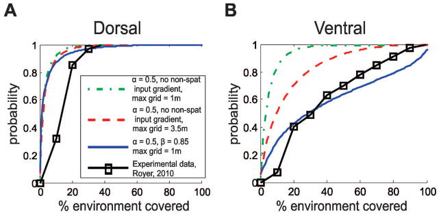
A Comparison of experimental and simulated cumulative distribution functions (CDFs) for dorsal place field sizes for 3 parameter sets. Experimental data (black lines, square markers) is adapted from Royer 2010, figure 2b. Green and red dashed lines show CDF plots with no non-spatial inputs and 2 different maximum grid scales (1m and 3.5m, respectively), while the blue dotted lines are CDF plots in the case where β = 0.85 and the maximum grid scale is 1m. B Comparison of experimental and simulated cumulative distribution functions for ventral place field sizes for 3 parameter sets. Line types are the same as in part A.

Winner-Take-All interactions must be confined to local portions of the dorsoventral axis

Our model discretizes the dorsoventral axis of the hippocampus into 50 sup-populations, and assumes that the winner-take-all inhibitory interactions that mediate place field formation occur predominately locally, within sub-populations that have similar input statistics with respect to grid scale and the amount of non-spatial input. However, it is possible that there is some overlap in the inhibitory interactions between groups at different dorsoventral levels (and with different input statistics), so we test the effect that introducing different levels of overlap has on place cell activity at different dorsoventral locations.

Figure 6 shows the effect of different amounts of overlap on the number of active place cells across the dorsoventral axis. Here α = 0.5 and β = 0.85 for all conditions. We see that even for moderate amounts of overlap (20%), there is a tendency for dorsal place cells to be less active than ventral cells, and that this effect becomes more important with increasing levels of overlap. This is in conflict with some experimental data, which suggests that an equivalent or higher number of dorsal cells than ventral cells have place fields in a given environment (Jung et al., 1994). This suppression of dorsal activity in the presence of overlap is due simply to the fact that the dorsoventral gradient in non-spatial input causes the more ventral place cell groups to have more overall excitation. When large overlaps exist, this puts ventral groups at an advantage over more dorsal groups in the winner-take-all competition, leading to the suppression of dorsal firing. As a result, we conclude that winner-take all dynamics coupled with a dorsoventral gradient in non-spatial excitation can only yield realistic levels of dorsal activity if the winner-take-all activity is predominantly local.

Note, however that this effect depends on the existence of a dorsoventral gradient in non-spatial excitation. If such a gradient does not exist, and there is no difference in the overall excitatory input between two neighboring place cell groups, then there will be no suppressive effect of the more ventral place cells upon the more dorsal place cells, and hence no effect on the proportion of active dorsal cells (results not shown).

Input variability affects place cell properties

Another factor that may have a significant influence on place cell properties is the amount of firing rate variance received by place cells. This amount of variance is experimentally unknown, but relates to the activity of areas such as the amygdala, ventral tegmental area or hypothalamus and hence may undergo significant changes. Here, we report the effect of changing this parameter while keeping the dorsoventral gradient in the mean non-spatial input the same.

First recall that the parameter controlling the width of the uniform distribution of non-spatial cell activities is the maximum firing rate NS_max (see Methods). However, changing NS_max not only changes the variance of the distribution, but also shifts the mean. To keep the mean fixed while changing the variance, the number N_nonspat,m (see equation 2) of non-spatial inputs to each place cell is scaled in proportion to NS_max, so that the average non-spatial excitation is kept fixed at some pre-specified value. In this way, the variance in the pool of non-spatial cells can be changed without affecting the mean total excitation to each cell: when NS_max is low, place cells receive a large number of weak inputs, and there is relatively little variance in the total input received by each individual place cell, whereas when the NS_max is high, place cells receive fewer total inputs which can range from weak to strong, leading to more variance in the amount of non-spatial excitation across the place cell population.

In Figure 7, we summarize the result of changing NS_max while keeping the mean non-spatial input constant as described above. We found that for both the high variance (NS_max = 5, corresponding to a variance of 25/12) and low-variance (NS_max = 0.5, corresponding to a variance of 0.25/12) cases, the introduction of non-spatial inputs produced a gradient in place field sizes, as expected (Figure 7A). Additionally, the total number of active ventral cells was much lower when there was more variance in the non-spatial inputs than when there was less variance (Figure 7B). Therefore, we conclude that the main effect of variance is to control the proportion of active ventral cells. The low variance case is equivalent to increasing the excitability of all ventral cells by the same amount, resulting in more overall activity and larger fields. On the other hand, the high variance case produces more cells that fail to “win” the winner take all competition and therefore do not fire. Additionally, the cells that do fire in this case tend to do so over a larger region of space, because of the spatially-uniform nature of the inputs that cause them to win out over other cells.

Variability in the properties of the spatial inputs to place cells promotes single place fields

In all current models describing the transformation of grid cell inputs into place cell firing patterns, the firing rates at all grid nodes are assumed to be identical. In contrast, experimental recordings of grid cells typically show substantial heterogeneity in the firing rates of the different grid nodes of the same grid cell (see Figure 9A, top) (Hafting et al., 2005). We next study how this heterogeneity affects place field formation and stability, and therefore introduce it into our model grid fields (see Figure 8A, bottom).

Figure 9. Response of place cell representation to changing non-spatial inputs.

A Randomly shuffling the firing rates of non-spatial cells results in place cell turnover across the entire DV axis. This shows the average percentage of cells that are active with both sets of contextual input values. B Spatial correlation of place fields in the two conditions, for cells that have place fields in both conditions.

We observed that when all of the grid cell inputs share the same spatial scale and orientation (i.e., when α ~ 0), the model tends to produce place cells with grid-like firing fields (Figure 8B, top left) instead of well-defined single place fields. If grid node firing rates are assumed to be uniform, the only way to introduce variance in spatial scale and/or orientation is by distributing the inputs to a place cell across many different grid cell modules. However, another source of variability in the properties of the grid cell inputs to place cells is variability into the grid node firing rates of individual grid fields. Such variability is consistently experimentally observed (Figure 8A, top) (Hafting et al., 2005), but is typically not included in models of the input-output relationship between grid cells and place cells (de Almeida et al., 2009a; McNaughton et al., 2006; Solstad et al., 2006).

Here we examined the effect of systematically increasing the node-to-node variability in individual grid fields by incrementally varying the parameter ξ, both in the case of zero variability in orientation and scale of grid inputs, and moderate variability, for a single place cell sub-group. We have found that increasing the variability in grid node firing rates increases the proportion of place cells with single place fields, especially in the absence of any variability in the spatial scale or orientation of the inputs (Figure 8C). However, when this variability in scale and orientation is already present (corresponding to higher values of α), increasing grid node variability has much less of an effect on place cell properties, indicating that some sort of variability in the spatial properties of grid cell inputs (either in terms of spatial scale, field orientation, or grid vertex firing rate) is important for generating place cells with single, well defined place fields.

Effect of grid geometry

A basic question is the degree to which observed place field properties depend on the precise geometry of grid cell firing patterns. Indeed, some recent experimental evidence has suggested that individual grid fields are elliptical rather than circular, and that the long axes of these elliptical grid fields are oriented in the same direction for an individual cell. Furthermore, the evidence indicates that anatomically nearby grid cells have elliptical grid fields oriented in a common direction (Stensola et al., 2012). To test whether such deviations from circular grid fields has any effect on place field properties, we ran a number of simulations using elliptical grid fields (Supplemental Figure S5A), and found that the inclusion of ellipticity had no discernible effect on the output of the model. Therefore, for simplicity we used circular grid fields in all other simulations discussed here.

Strikingly, in a second set of simulations, we observed that we could disrupt the grid geometry entirely (while preserving the amount of overall spatial modulation) and still obtain valid place fields (Supplemental Figure S5B). This indicates that the regular-grid-like pattern of nodes that characterize grid cells is not important for the generation of place fields in our model, and that the WTA model of place field formation only requires some sort of spatial modulation in the inputs as a prerequisite for forming place fields. The significance of the regular arrangement of the nodes (if any) for place field expression remains to be fully elucidated, although theoretical work has suggested that the hexagonal arrangement may be advantageous for encoding position, independently of place cells (Fiete et al., 2008; Sreenivasan and Fiete, 2011).

Sensitivity of place fields to changes in non-spatial inputs and grid node firing rates

Place cells can remap due to changes in the non-spatial inputs

Our simulations model the non-spatial inputs to place cells as fixed, tonic firing rates, while in reality it is possible that the firing rates of these non-spatial cells could change as a result of contextual or emotional changes. We conducted simulations to assess how changing only the non-spatial inputs to place cells could lead to place cell remapping. For a single network, we generated a set of place fields using a particular set of firing rates for the non-spatial cells. We then generated a second set of place fields using a second set of non-spatial firing rates (drawn from the same distribution), but keeping all connection weights and grid cell properties identical to the original network. We then assessed the amount of cell turnover and the spatial correlation between place fields generated in the two conditions. This was repeated across 20 independent networks with identical statistical properties.

We found that cell turnover was significant, (Figure 9A) implying that the non-spatial inputs play an important role in selecting which cells fire. This also suggests that fluctuations in the firing rates of non-spatial cells will reduce the stability of place fields. There was also a loss of spatial correlation the cells that were active in both conditions, although there was considerable variance in the correlation values (Figure 9B).

Dorsal place fields are sensitive to changes in grid node firing rate patterns

Because our simulations use grid cells with realistically variable grid node firing rates, we investigated whether perturbing the patterns of grid node firing rates while fixing the geometric properties of the grid cells (scale, orientation and phase) could induce remapping in the downstream place cell populations. To do so, we first generated two populations of grid cells with identical geometric properties, but independently chosen patterns of grid node firing rates. We then assessed the degree of remapping between the two resulting place cell populations, using the remapping measures described in a previous section on the analysis of model output.

Figure 10 shows the change in the place fields as a function of grid node remapping, using the two measures of place field remapping. Here we set α = 0.5, β = 0.85, and ξ = 0.5 to remain consistent with the previous simulations. Figures 10A and 10B show the cell turnover and spatial correlation respectively for place fields across the dorsoventral axis between the place fields generated using the two sets of grid patterns. These results suggest that the dorsal-most place cells can globally remap due to changes in the grid node firing rate patterns of their grid cell inputs, even when the phase and orientation of all of the grid patterns remains fixed.

Figure 10. Response of place cell representation to changes in grid node firing rate variability.

A Proportion of shared active cells for two independently generated sets of grid node firing rate patterns at different dorsoventral locations, showing significant cell turnover in the dorsal hippocampus as a result of changes in just the firing rates of individual grid nodes. The phases, orientations and spatial scales of all grid cells are identical in both conditions. B Spatial decorrelation of place field maps between the two conditions.

In addition, our model suggests that the remapping due to grid node fluctuations should be less pronounced at more ventral locations, since the properties of these ventral cells are dominated by non-spatial inputs. Since dorsal place cells are more stable over the timescale of a single recording session (Royer et al., 2010), this could imply that either grid node firing rate patterns are stable over time (and perhaps carry some coding significance), or that some external mechanism is responsible for keeping dorsal place fields stable in the face of such fluctuations.

Discussion

Our modeling work is different from prior studies in a number of ways. First, we organized both grid cells and place cells on the basis of spatial scale, and systematically varied the degree of spatial scale selectivity in the grid cell inputs to place cells (Lyttle, 2012). Secondly, we introduced a dorsoventral gradient in the non-spatial inputs to place cells, with ventral cells receiving more input from non-spatial sources. Because there are likely to be multiple sources of non-spatial inputs to the ventral hippocampus, we did not specify a single anatomical source for these inputs. Rather, we assumed they represented some combination of contextual, non-spatial and emotional inputs from sources including the amygdala, hypothalamus, and ventral tegmental area. One previous computational study explored the role of (low spatial information content) LEC inputs on place cell rate remapping (Renno-Costa et al., 2010), however they did not compare the relative effects of grid scale and non-spatial inputs on place cell properties along the dorsoventral axis. Finally, we introduced heterogeneity in the firing rates of grid vertices within individual grid fields. This heterogeneity is observed in experiments but has received relatively little attention in either experimental or theoretical work, despite its potential impact on position estimation as well as the stability and formation of place fields.

The relative contributions of grid field scale and non-spatial inputs in determining place field size

A central result of our study is that place field size is strongly influenced by the degree of spatial specificity in the inputs to place cells, and is affected less strongly by the spatial scale of grid cell inputs. This suggests that the dorsoventral gradient in place field size may reflect a gradual change in the type of information being processed by the hippocampus, with the dorsal hippocampus processing primarily spatial location-dependent information, and the ventral hippocampus processing broader contextual and emotional information. This agrees with experimental findings that have suggested that the dorsal and ventral hippocampal regions may be functionally distinct and process different types of information. Early evidence to this effect was found in selective hippocampal lesioning studies where selective lesions to the dorsal hippocampus produced deficits in spatial memory and navigation, whereas lesions of the ventral hippocampus did not affect spatial navigation, but instead produced deficits in fear conditioning (Czerniawski et al., 2009; Kjelstrup et al., 2002; Steffenach et al., 2005). A particularly relevant recent study found fundamental differences in spatial representation between dorsal and ventral CA3 cells (Royer et al., 2010). Specifically, ventral cells showed higher reward sensitivity, and were able to distinguish between the inbound and outbound directions of travel and between the open and closed arms of a maze in a radial maze task more effectively than dorsal cells. Finally, recent fMRI studies in humans suggest that there may be functional differences between the anterior and posterior portions of the hippocampus (Poppenk et al., 2013). Collectively, these results suggest that the dorsal and ventral portions of the hippocampus are functionally distinct, and our modeling results suggest that the differences in place field size may simply reflect this functional distinction.

Ultimately, more detailed anatomical studies of the various input projections to the hippocampus will be required to determine the respective contributions of grid cells and non-spatial input sources in producing the dorsoventral gradient in place field size. Our model predicts that strict topographical organization in the grid-to-place connectivity (i.e. a low value of α) along with the existence of very large grids in a 2D environment are necessary for the scale of grid inputs to have an important role in determining place field size. On the other hand, if place field size is largely determined by the relative amounts of spatial and non-spatial inputs, then there should be a dorsoventral gradient in either the density or strength of incoming connections from cells that show little to no spatial modulation. We also predict that selectively lesioning the dorsal entorhinal cortex will result in an increase in dorsal place field size, but that selectively lesioning the ventral entorhinal cortex will have very little effect on dorsal place field size (see Supplemental Figure S2). The inclusion of non-spatial inputs in our model was motivated by anatomical evidence suggesting that the ventral hippocampus preferentially receives non-spatial and emotional inputs from areas such as the amygdala, hypothalamus, and VTA (Petrovich et al., 2001; Risold and Swanson, 1996; Witter et al., 1989); Precisely pinpointing the dominant sources of non-spatial inputs to the ventral hippocampus and selectively lesioning them while assessing the impact on ventral place field size could provide a direct test of the results of our model, which predicts an average decrease in ventral place field size in the absence of additional non-spatial inputs.

If place field size is in fact not solely a function of the spatial scale of a place cell’s grid cell inputs, then an interesting question arises as to what computational advantages exist, if any, in a multi-scale representation of space in entorhinal grid cells. One possibility is that spatial navigation in the face of environmental changes at a specific spatial scale may be more robust if spatial information at other scales is present. Further work will be required to better understand the functional significance of representing space at multiple scales.

It is important to note that while our findings highlight the role of non-spatial inputs in determining place field size, the present model cannot rule out the possibility that intrinsic cellular properties or some factor other than non-spatial inputs may also be involved in producing the observed dorsoventral gradient in place field size. Recent experimental work involving HCN1 knockout mice has produced evidence that this channel is involved in setting the spatial scale of both grid cells (Giocomo et al., 2011) and place cells (Hussaini et al., 2011). Interestingly, while the grid fields were larger in the HCN1 knockouts, the dorsoventral gradient in grid scale was preserved (Giocomo et al., 2011). The corresponding study in place cells only involved recordings at a single dorsoventral location (Hussaini et al., 2011), and thus it is not currently known whether a dorsoventral gradient in place field size is present in HCN1 knockout mice. We observe however, that the effective role of the non-spatial inputs in our model is to produce a dorsoventral gradient in the spatially-independent excitability of cells. This change in excitability could also be the result of a dorsoventral gradient in intracellular properties (Dougherty et al., 2012; Dougherty et al., 2013), and would yield similar if not identical place field to those observed in our model. Our assumption that the changes in excitability are due to non-spatial input is motivated by anatomical differences in the projections to the dorsal and ventral hippocampus, but careful experimental work will be required to distinguish the effects of external inputs from intrinsic intracellular differences. In either case, however, the observed dorsoventral differences in place field properties would be due to factors other than the change in spatial scale of grid fields.

It has also been proposed that the spatial properties of dorsal place fields may be tightly linked to the presence of theta oscillations in the rat (Maurer et al., 2005; O’Keefe and Burgess, 2005; Tsodyks et al., 1996). This finding is compatible with recent observations that ventral place fields are larger, often much more difficult to define, and also have very weak theta oscillation (Patel et al., 2012; Royer et al., 2010). However, the relationship between theta and place field spatial properties has recently been challenged by studies in bats, in which well-defined place fields can be found even though theta oscillations are absent, whether the bats fly or crawl (Ulanovsky and Moss, 2011; Yartsev et al., 2011). Our modeling results suggest that the poor spatial selectivity of ventral place fields may be mainly due to the presence of a high amount of non-spatial input, and that the fact that theta is absent in the ventral hippocampus may be unrelated to spatial selectivity.

Local winner take all interactions are consistent with normal place field expression

In constructing our model, we discretize the dorsoventral axis of the hippocampus into smaller groups of place cells representing different dorsoventral locations. The winner-take-all competition which shapes place fields in our model is confined to within these groups. We explored the effects of increasing the amount of overlap between nearby groups, and found that with significant overlap, more ventral place cells tended to dominate due to increased levels of excitation, and suppressed the firing of dorsal cells. This predicts that if a dorsoventral gradient in non-spatial input is present, winner-take-all competition must take place within subpopulations of place cells with similar input statistics in order to produce realistic levels of dorsal place cell activity, implying that lateral inhibition must only extend across a fraction of the dorsoventral axis. This is quite reasonable, and consistent with known hippocampal anatomy. In particular, inhibitory basket cells are one of the more common cell types in the hippocampus that could serve to mediate winner-take-all interactions, and their spatial extent is limited to a small fraction of the dorsoventral axis of the hippocampus (Freund and Buzsaki, 1996). However more work must be done to assess the strength and functional role of longer-rage inhibitory interactions across different dorsoventral distances, in order to determine if our predictions are accurate.

Effect of input variance and geometry

Another finding of this work is that increased variability in the firing rates of non-spatial cells decreases the number of active ventral cells. In other words, in the context of the winner-take-all mechanism for place cell formation, a richer and more diverse set of non-spatial inputs is associated with sparser activity in the ventral hippocampus. Consequently, greater non-spatial or emotional complexity in an environment may be associated with sparser ventral coding. Detailed measurements of the proportion of cells with place fields in the ventral hippocampus would help determine which of these two mechanisms is more likely to be involved in setting place field size, although existing data suggests that there are slightly fewer ventral place cells than dorsal place cells active in a given environment (Jung et al., 1994; Royer et al., 2010).

Additionally, our simulations involving elliptical and randomized grid cell inputs suggest that the degree of spatial modulation in the inputs to place cells may be more important than the precise grid geometry of those inputs for producing place fields. This implies that place fields can form without input from medial entorhinal grid cells, provided that they receive some sort of spatially modulated input. This idea is consistent with the experimental observations that place fields are observable earlier in development than grid fields (Wills et al., 2010) and that place fields persist after disruption of entorhinal grid cells firing (Koenig et al., 2011). Furthermore, our model predicts that under experimental conditions such as these, where grid cells are disabled but place cells still persist, the dorsoventral gradient should still be apparent. Finally, we note that there are other candidate sources of spatially modulated input to place cells, such as border cells, and even weakly-spatial input from the lateral entorhinal cortex may be sufficient to induce place field formation, given that place fields are observed in the distal hippocampus, which receives primarily lateral entorhinal input (Henriksen et al., 2010).

Place cell stability

In addition to studying the respective roles of spatial and non-spatial inputs in determining place field size, we studied how these different types of inputs affect place field stability. We found that non-spatial inputs can affect the stability of place fields, and may play a role in selecting which place cells fire, consistent with recent experimental findings indicating that the injection of a spatially uniform current into place cells causes them to develop place fields in an environment in which they previously were inactive (Lee et al., 2012).

Another set of results concerns the stability of place fields in the face of grid cell firing rate fluctuations. Firing rate heterogeneity in the grid vertices of grid cells, despite being an experimental fact (Hafting et al., 2005), has received relatively little attention. The apparent sensitivity of dorsal place fields to variations in the node-to-node patterns of grid cell firing rates raises several questions. An important question is whether these heterogeneous firing rate patterns remain stable over behaviorally relevant timescales. If they do, then one may ask if these patterns reflect some sort of external modulation, and if they have any functional or coding significance, as one recent study has suggested (Reifenstein et al., 2012). Alternatively, if the firing rates of individual grid nodes are not stable over time, then the apparent temporal stability of place fields requires further explanation. Further experimental work will be required to precisely quantify the temporal stability of the grid field firing rates and to measure the magnitude of these fluctuations.

Role for network dynamics

Finally, we note that our model, like that of de Almeida et al, assumes that a static rate-based model is sufficient to capture the essential properties of the grid-to-place cell system. In ongoing work we are exploring the possibility that complex dynamical interactions can modulate or affect the stability of the system.

Table 1. Experimental data on ventral place field size.

Summary of recent experimental studies that indicate a dorsoventral increase in place field size.

Study	Kjelstrup, 2008	Royer2010
Environment type	Linear track, 18m	2-D open field, 2m2
Mean dorsal place field size	~5 % of environment	~18 % of environment
Mean ventral place field size	~27 % of environment	~42 % of environment
Increase in mean place field size	~5-fold increase in mean coverage	~2-fold increase in mean coverage

References

- Brun VH, Solstad T, Kjelstrup KB, Fyhn M, Witter MP, Moser EI, Moser MB. Progressive increase in grid scale from dorsal to ventral medial entorhinal cortex. Hippocampus. 2008;18(12):1200–12. doi: 10.1002/hipo.20504. [DOI] [PubMed] [Google Scholar]
- Czerniawski J, Yoon T, Otto T. Dissociating space and trace in dorsal and ventral hippocampus. Hippocampus. 2009;19(1):20–32. doi: 10.1002/hipo.20469. [DOI] [PubMed] [Google Scholar]
- de Almeida L, Idiart M, Lisman JE. The input-output transformation of the hippocampal granule cells: from grid cells to place fields. J Neurosci. 2009a;29(23):7504–12. doi: 10.1523/JNEUROSCI.6048-08.2009. [DOI] [PMC free article] [PubMed] [Google Scholar]
- de Almeida L, Idiart M, Lisman JE. A second function of gamma frequency oscillations: an E%-max winner-take-all mechanism selects which cells fire. J Neurosci. 2009b;29(23):7497–503. doi: 10.1523/JNEUROSCI.6044-08.2009. [DOI] [PMC free article] [PubMed] [Google Scholar]
- de Almeida L, Idiart M, Lisman JE. The single place fields of CA3 cells: A two-stage transformation from grid cells. Hippocampus. 2010 doi: 10.1002/hipo.20882. [DOI] [PMC free article] [PubMed] [Google Scholar]
- Dougherty KA, Islam T, Johnston D. Intrinsic excitability of CA1 pyramidal neurones from the rat dorsal and ventral hippocampus. J Physiol. 2012;590(Pt 22):5707–22. doi: 10.1113/jphysiol.2012.242693. [DOI] [PMC free article] [PubMed] [Google Scholar]
- Dougherty KA, Nicholson DA, Diaz LM, Buss EW, Neuman KM, Chetkovich DM, Johnston D. Differential Expression of HCN Subunits Alters Voltage-Dependent Gating of h-channels in CA1 Pyramidal Neurons from the Dorsal and Ventral Hippocampus. J Neurophysiol. 2013 doi: 10.1152/jn.00010.2013. [DOI] [PMC free article] [PubMed] [Google Scholar]
- Fiete IR, Burak Y, Brookings T. What grid cells convey about rat location. J Neurosci. 2008;28(27):6858–71. doi: 10.1523/JNEUROSCI.5684-07.2008. [DOI] [PMC free article] [PubMed] [Google Scholar]
- Freund TF, Buzsaki G. Interneurons of the hippocampus. Hippocampus. 1996;6(4):347–470. doi: 10.1002/(SICI)1098-1063(1996)6:4<347::AID-HIPO1>3.0.CO;2-I. [DOI] [PubMed] [Google Scholar]
- Fuhs MC, Touretzky DS. A spin glass model of path integration in rat medial entorhinal cortex. J Neurosci. 2006;26(16):4266–76. doi: 10.1523/JNEUROSCI.4353-05.2006. [DOI] [PMC free article] [PubMed] [Google Scholar]
- Gasbarri A, Sulli A, Packard MG. The dopaminergic mesencephalic projections to the hippocampal formation in the rat. Prog Neuropsychopharmacol Biol Psychiatry. 1997;21(1):1–22. doi: 10.1016/s0278-5846(96)00157-1. [DOI] [PubMed] [Google Scholar]
- Giocomo LM, Hussaini SA, Zheng F, Kandel ER, Moser MB, Moser EI. Grid cells use HCN1 channels for spatial scaling. Cell. 2011;147(5):1159–70. doi: 10.1016/j.cell.2011.08.051. [DOI] [PubMed] [Google Scholar]
- Hafting T, Fyhn M, Molden S, Moser MB, Moser EI. Microstructure of a spatial map in the entorhinal cortex. Nature. 2005;436(7052):801–6. doi: 10.1038/nature03721. [DOI] [PubMed] [Google Scholar]
- Hayman RM, Jeffery KJ. How heterogeneous place cell responding arises from homogeneous grids--a contextual gating hypothesis. Hippocampus. 2008;18(12):1301–13. doi: 10.1002/hipo.20513. [DOI] [PubMed] [Google Scholar]
- Henriksen EJ, Colgin LL, Barnes CA, Witter MP, Moser MB, Moser EI. Spatial representation along the proximodistal axis of CA1. Neuron. 2010;68(1):127–37. doi: 10.1016/j.neuron.2010.08.042. [DOI] [PMC free article] [PubMed] [Google Scholar]
- Hussaini SA, Kempadoo KA, Thuault SJ, Siegelbaum SA, Kandel ER. Increased size and stability of CA1 and CA3 place fields in HCN1 knockout mice. Neuron. 2011;72(4):643–53. doi: 10.1016/j.neuron.2011.09.007. [DOI] [PMC free article] [PubMed] [Google Scholar]
- Jung MW, Wiener SI, McNaughton BL. Comparison of spatial firing characteristics of units in dorsal and ventral hippocampus of the rat. J Neurosci. 1994;14(12):7347–56. doi: 10.1523/JNEUROSCI.14-12-07347.1994. [DOI] [PMC free article] [PubMed] [Google Scholar]
- Kjelstrup KB, Solstad T, Brun VH, Hafting T, Leutgeb S, Witter MP, Moser EI, Moser MB. Finite scale of spatial representation in the hippocampus. Science. 2008;321(5885):140–3. doi: 10.1126/science.1157086. [DOI] [PubMed] [Google Scholar]
- Kjelstrup KG, Tuvnes FA, Steffenach HA, Murison R, Moser EI, Moser MB. Reduced fear expression after lesions of the ventral hippocampus. Proc Natl Acad Sci U S A. 2002;99(16):10825–30. doi: 10.1073/pnas.152112399. [DOI] [PMC free article] [PubMed] [Google Scholar]
- Koenig J, Linder AN, Leutgeb JK, Leutgeb S. The spatial periodicity of grid cells is not sustained during reduced theta oscillations. Science. 2011;332(6029):592–5. doi: 10.1126/science.1201685. [DOI] [PubMed] [Google Scholar]
- Lyttle D, Lin K, Fellous JM. Coding stability, and non-spatial inputs in a modular grid-to-place cell model. Atlanta: 2012. [Google Scholar]
- Maurer AP, Vanrhoads SR, Sutherland GR, Lipa P, McNaughton BL. Self-motion and the origin of differential spatial scaling along the septo-temporal axis of the hippocampus. Hippocampus. 2005;15(7):841–52. doi: 10.1002/hipo.20114. [DOI] [PubMed] [Google Scholar]
- McNaughton BL, Battaglia FP, Jensen O, Moser EI, Moser MB. Path integration and the neural basis of the ‘cognitive map’. Nat Rev Neurosci. 2006;7(8):663–78. doi: 10.1038/nrn1932. [DOI] [PubMed] [Google Scholar]
- Monaco JD, Abbott LF. Modular realignment of entorhinal grid cell activity as a basis for hippocampal remapping. J Neurosci. 2011;31(25):9414–25. doi: 10.1523/JNEUROSCI.1433-11.2011. [DOI] [PMC free article] [PubMed] [Google Scholar]
- Moser EI, Kropff E, Moser MB. Place cells, grid cells, and the brain’s spatial representation system. Annu Rev Neurosci. 2008;31:69–89. doi: 10.1146/annurev.neuro.31.061307.090723. [DOI] [PubMed] [Google Scholar]
- O’Keefe J. Place units in the hippocampus of the freely moving rat. Exp Neurol. 1976;51(1):78–109. doi: 10.1016/0014-4886(76)90055-8. [DOI] [PubMed] [Google Scholar]
- O’Keefe J, Burgess N. Geometric determinants of the place fields of hippocampal neurons. Nature. 1996;381(6581):425–8. doi: 10.1038/381425a0. [DOI] [PubMed] [Google Scholar]
- O’Keefe J, Burgess N. Dual phase and rate coding in hippocampal place cells: theoretical significance and relationship to entorhinal grid cells. Hippocampus. 2005;15(7):853–66. doi: 10.1002/hipo.20115. [DOI] [PMC free article] [PubMed] [Google Scholar]
- Patel J, Fujisawa S, Berenyi A, Royer S, Buzsaki G. Traveling theta waves along the entire septotemporal axis of the hippocampus. Neuron. 2012;75(3):410–7. doi: 10.1016/j.neuron.2012.07.015. [DOI] [PMC free article] [PubMed] [Google Scholar]
- Petrovich GD, Canteras NS, Swanson LW. Combinatorial amygdalar inputs to hippocampal domains and hypothalamic behavior systems. Brain Res Brain Res Rev. 2001;38(1–2):247–89. doi: 10.1016/s0165-0173(01)00080-7. [DOI] [PubMed] [Google Scholar]
- Poppenk J, Evensmoen H, Moscovitch M, Nadel L. Long-axis specialization of the human hippocampus. 2013 doi: 10.1016/j.tics.2013.03.005. Submitted. [DOI] [PubMed] [Google Scholar]
- Reifenstein ET, Kempter R, Schreiber S, Stemmler MB, Herz AV. Grid cells in rat entorhinal cortex encode physical space with independent firing fields and phase precession at the single-trial level. Proc Natl Acad Sci U S A. 2012;109(16):6301–6. doi: 10.1073/pnas.1109599109. [DOI] [PMC free article] [PubMed] [Google Scholar]
- Renno-Costa C, Lisman JE, Verschure PF. The mechanism of rate remapping in the dentate gyrus. Neuron. 2010;68(6):1051–8. doi: 10.1016/j.neuron.2010.11.024. [DOI] [PMC free article] [PubMed] [Google Scholar]
- Risold PY, Swanson LW. Structural evidence for functional domains in the rat hippocampus. Science. 1996;272(5267):1484–6. doi: 10.1126/science.272.5267.1484. [DOI] [PubMed] [Google Scholar]
- Royer S, Sirota A, Patel J, Buzsaki G. Distinct representations and theta dynamics in dorsal and ventral hippocampus. J Neurosci. 2010;30(5):1777–87. doi: 10.1523/JNEUROSCI.4681-09.2010. [DOI] [PMC free article] [PubMed] [Google Scholar]
- Si B, Treves A. The role of competitive learning in the generation of DG fields from EC inputs. Cogn Neurodyn. 2009;3(2):177–87. doi: 10.1007/s11571-009-9079-z. [DOI] [PMC free article] [PubMed] [Google Scholar]
- Solstad T, Moser EI, Einevoll GT. From grid cells to place cells: a mathematical model. Hippocampus. 2006;16(12):1026–31. doi: 10.1002/hipo.20244. [DOI] [PubMed] [Google Scholar]
- Sreenivasan S, Fiete I. Grid cells generate an analog error-correcting code for singularly precise neural computation. Nat Neurosci. 2011;14(10):1330–7. doi: 10.1038/nn.2901. [DOI] [PubMed] [Google Scholar]
- Steffenach HA, Witter M, Moser MB, Moser EI. Spatial memory in the rat requires the dorsolateral band of the entorhinal cortex. Neuron. 2005;45(2):301–13. doi: 10.1016/j.neuron.2004.12.044. [DOI] [PubMed] [Google Scholar]
- Stensola H, Stensola T, Solstad T, Froland K, Moser MB, Moser EI. The entorhinal grid map is discretized. Nature. 2012;492(7427):72–8. doi: 10.1038/nature11649. [DOI] [PubMed] [Google Scholar]
- Tsodyks MV, Skaggs WE, Sejnowski TJ, McNaughton BL. Population dynamics and theta rhythm phase precession of hippocampal place cell firing: a spiking neuron model. Hippocampus. 1996;6(3):271–80. doi: 10.1002/(SICI)1098-1063(1996)6:3<271::AID-HIPO5>3.0.CO;2-Q. [DOI] [PubMed] [Google Scholar]
- Ulanovsky N, Moss CF. Dynamics of hippocampal spatial representation in echolocating bats. Hippocampus. 2011;21(2):150–61. doi: 10.1002/hipo.20731. [DOI] [PMC free article] [PubMed] [Google Scholar]
- Wills TJ, Cacucci F, Burgess N, O’Keefe J. Development of the hippocampal cognitive map in preweanling rats. Science. 2010;328(5985):1573–6. doi: 10.1126/science.1188224. [DOI] [PMC free article] [PubMed] [Google Scholar]
- Witter MP, Groenewegen HJ, Lopes da Silva FH, Lohman AH. Functional organization of the extrinsic and intrinsic circuitry of the parahippocampal region. Prog Neurobiol. 1989;33(3):161–253. doi: 10.1016/0301-0082(89)90009-9. [DOI] [PubMed] [Google Scholar]
- Yartsev MM, Witter MP, Ulanovsky N. Grid cells without theta oscillations in the entorhinal cortex of bats. Nature. 2011;479(7371):103–7. doi: 10.1038/nature10583. [DOI] [PubMed] [Google Scholar]
Associated Data
This section collects any data citations, data availability statements, or supplementary materials included in this article.