Abstract
Recent theoretical results on low-rank matrix reconstruction have inspired significant interest in low-rank modeling of MRI images. Existing approaches have focused on higher-dimensional scenarios with data available from multiple channels, timepoints, or image contrasts. The present work demonstrates that single-channel, single-contrast, single-timepoint k-space data can also be mapped to low-rank matrices when the image has limited spatial support or slowly varying phase. Based on this, we develop a novel and flexible framework for constrained image reconstruction that uses low-rank matrix modeling of local k-space neighborhoods (LORAKS). A new regularization penalty and corresponding algorithm for promoting low-rank are also introduced. The potential of LORAKS is demonstrated with simulated and experimental data for a range of denoising and sparse-sampling applications. LORAKS is also compared against state-of-the-art methods like homodyne reconstruction, ℓ1-norm minimization, and total variation minimization, and is demonstrated to have distinct features and advantages. In addition, while calibration-based support and phase constraints are commonly used in existing methods, the LORAKS framework enables calibrationless use of these constraints.
Index Terms: Low-Rank Matrix Recovery, Constrained Image Reconstruction, Phase Constraints, Support Constraints
I. Introduction
Constrained reconstruction is increasingly common in MRI because it offers capabilities to reduce k-space sampling requirements, reduce noise confounds, and correct artifacts (see, e.g., [1], [2] and references). Such approaches are enabled by the substantial structure present in MR images, which can be exploited to compensate for incomplete/low-quality data. While various constraints have been proposed, many approaches implicitly rely on linear dependence relationships.
A set of vectors is said to be linearly dependent if there exists a set of scalars (not all zero) such that
| (1) |
Linear dependence relationships imply that
| (2) |
for each p ∈ {1, …, N} with αp ≠ 0. In other words, linear dependence relationships mean that vectors can be predicted from each other. Such relationships enable both reduced data acquisition (e.g., xp need not be sampled if it can be predicted from the other vectors) and noise reduction (e.g., the ability to average xp with its value predicted from the other xn).
An incomplete list of constrained MR imaging methods that exploit linear dependence relationships includes: parallel imaging methods like GRAPPA [3], SPIRiT [4], and PRUNO [5] that exploit linear dependencies between k-space samples from different receiver coils within local k-space neighborhoods; autoregressive moving average (ARMA) linear prediction models of Fourier data [6]–[9]; feature-recognizing MRI [10], [11], which can be interpreted as learning linear dependence relationships from a database of training images; support-limited reconstruction methods [12]–[16]; partially separable function models of dynamic imaging data [17], [18], in which the temporal variations from different spatial locations in the dynamic image are assumed to be linearly dependent; and phase-constrained partial Fourier reconstruction techniques that rely on the Fourier symmetry characteristics of images with slowly varying phase [19]–[21]. All of these methods rely on knowledge of the linear dependence coefficients , which have generally been derived from calibration data: fully sampled k-space regions that can be used to estimate .
In recent years, calibrationless generalizations of some of these methods have been proposed based on techniques from the emerging theory of low-rank matrix recovery [22], which itself is a generalization of the theory of sparsity-based compressed sensing [23], [24]. In particular, calibrationless matrix recovery methods have emerged to exploit linear dependencies in applications like dynamic imaging [2], [25]–[33], parallel imaging [34]–[36], spectroscopic imaging [37], [38], diffusion imaging [2], [39]–[41], and functional imaging [42], [43]. Compared to calibration-based methods, calibrationless low-rank methods have the advantages that: (1) they enable the use of more general sampling schemes; (2) they estimate linear dependence structure using the entire set of measured data, instead of just the subset of calibration data; and (3) they are immune to mismatches between the prior information and imaging data that might arise (e.g., due to subject motion, B0 field drift, etc.) if the calibration data is acquired in a prescan.
In contrast to previous calibrationless methods, which have largely focused on low-rank modeling in high-dimensional imaging scenarios with multiple channels, contrasts, or timepoints, the present work proposes a new framework for low-rank modeling of local k-space neighborhoods (LORAKS) that is applicable to low-dimensional single-channel, single-contrast, single-timepoint images. This is achieved by mapping lower-dimensional images into higher-dimensional matrices in novel ways, based on linear dependencies that are present in the k-space data of images with limited spatial support and/or slowly varying phase. LORAKS is very flexible, and is easily used in combination with other constraints. Moreover, LORAKS imposes support and phase constraints in a fundamentally different way from more direct regularized methods [44], [45], and can provide information that is distinct from and potentially complementary to such approaches. A preliminary account of part of this work was presented in [46].
We are aware of only two other low-rank image reconstruction methods that have been proposed for calibrationless low-rank reconstruction of individual MRI images [47], [48], and neither of these approaches were designed to impose phase or support constraints. Specifically, [47] is based on generic ARMA modeling assumptions [6]–[9], while [48] is related to feature-recognizing MRI [10], [11], and uses the assumptions of singular value decomposition (SVD) image coding [49].
This paper is organized as follows. Section II describes several k-space linear dependence relationships that are used to construct low-rank matrices. Section III discusses low-rank matrix reconstruction and introduces a new penalty function and algorithm for this problem. Section IV illustrates the application of LORAKS to a variety of experimental datasets. We finish with discussion and conclusions in section V.
II. Linear Dependence Relationships in k-Space
The following subsections derive and demonstrate the construction of low-rank matrices based on support and phase constraints. Without loss of generality, we will consider a 2D imaging scenario with the image denoted by ρ(x, y).
A. Linear Dependencies Induced by Limited Image Support
We define the support of ρ(x, y) as the set of points Ωρ = {(x, y) ∈ ℝ2: |ρ(x, y)| ≠ 0}. The use of support information is universal in MRI, since the size and shape of the image support determines how the imaging field of view (FOV) and the corresponding Nyquist sampling rate are chosen. However, an important observation is that k-space data sampled at the Nyquist rate will have linear dependencies whenever there are measurable regions within the FOV for which ρ(x, y) = 0 [12]. To see this, consider any non-zero function f (x, y) which obeys both Ωf ⊂ FOV and f (x, y) = 0 for ∀ (x, y) ∈ Ωρ, and note that ρ(x, y) f (x, y) = 0 for ∀(x, y) ∈ ℝ2. If we denote the Nyquist-sampled Fourier transforms of ρ(x, y) and f (x, y) as ρ̃[nx, ny] and f̃[nx, ny], respectively, then the convolution theorem of the Fourier transform leads to
| (3) |
for ∀(nx, ny) ∈ ℤ2.
This expression demonstrates redundancies in Nyquist-sampled k-space data. However, these redundancies are difficult to use because the sums are infinite. This is resolvable if we further assume that there exist smooth functions f (x, y) satisfying f (x, y) = 0 for ∀(x, y) ∈ Ωρ, since smooth functions are approximated accurately using Fourier truncation. In this work, we assume that functions exist with f̃[nx, ny] ≈ 0 whenever (nx, ny) ∉ ΛR, where is the set of points within radius R of the origin. Letting NR denote the number of elements in ΛR and assuming that these elements have been assigned an (arbitrary) order such that the point (pm, qm) corresponds to the mth element of ΛR, (3) simplifies to
| (4) |
for ∀(nx, ny) ∈ ℤ2.
B. Low-Rank Matrices and Limited Image Support
The relationship in (4) can be exploited to construct an approximately rank-deficient matrix C from Nyquist-sampled k-space data. In particular, if we arbitrarily select K distinct k-space points indexed by
with K ≥ NR, then (4) implies that the matrix C ∈
 with elements
| (5) |
for k = 1, …, K and m = 1, …, NR will have
| (6) |
for all vectors f̃ ∈
 obtained from the Nyquist-sampled Fourier transforms of appropriate f (x, y) functions. Note that each row of C collects the set of k-space points from a local neighborhood of radius R, centered at (
).
In practice, the approximate rank of C will depend on the size of the approximate nullspace of C, which depends on R and the size of Ωρ relative to the FOV. The dependence on R results from the fact that larger R values would permit f (x, y) functions with higher spatial resolution. Having access to higher resolution f (x, y) functions would increase the dimension of the nullspace, since it would become possible to include more highly localized functions f (x, y) that could fit into small gaps and/or be tiled across larger gaps in the image support. Note also that the size of the matrix C will grow in proportion to R2, since NR ∝ R2. This implies that larger R can be associated with larger computation requirements.
C. Empirical Validation of the Characteristics of C
To validate these ideas, we performed a simple simulation involving the Shepp-Logan phantom. Specifically, we used analytic Fourier transform expressions [50] to simulate k-space data sampled on a 256 × 256 Cartesian grid, for different values of the k-space sampling rate Δk. A normalized value of Δk = 1 corresponds to the Nyquist rate, and we also generated data for Δk = 1/2, 1/3, 1/4, and 1/5. Note that smaller values of Δk correspond to larger imaging FOVs in the reconstructed images, such that the size of Ωρ shrinks in relation to the FOV. These simulated images are shown in Fig. 1.1
Fig. 1.

Images reconstructed using simulated 256 × 256 Cartesian Fourier data acquired with different Δk values.
To test our predictions about matrix rank, we computed SVDs of C matrices constructed from these simulated datasets. The SVD decomposes the matrix C ∈
 with K ≥ NR according to C = UΣVH, where U ∈
 and V ∈
 are matrices with orthonormal columns, and Σ ∈ ℝNR×NR is a diagonal matrix whose diagonal entries σk for k = 1, …, NR are ordered such that σ1 ≥ σ2 ≥ … ≥ σNR ≥ 0. The rank of C is equal to the number of nonzero singular values, and matrices with many negligible singular values are accurately approximated by low-rank matrices.
For this set of simulations, we chose K = (256 − 2R)2, which was the maximum number of k-space points that had their entire neighborhood system contained within the 256 × 256 sampling grid.2 We also considered several different neighborhood systems ΛR corresponding to different values of the k-space radius, i.e., R = 1, 2, 3, and 5, which yield NR = 5, 13, 29, and 81, respectively. These different k-space neighborhood systems are illustrated in Fig. 2.
Fig. 2.

Neighborhood systems for different k-space neighborhood radii R, with the centers of the neighborhood systems marked in red.
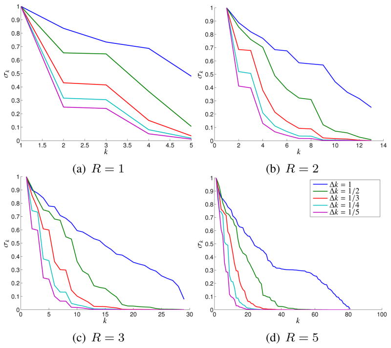
Figure 3 shows plots of the singular values obtained for different values of Δk and R (normalized such that the maximum singular value σ1 equals 1). As expected, the singular values decay more rapidly for smaller values of Δk, indicating that C matrices generated from images with smaller support are more easily approximated by low-rank matrices. In addition, we observe that increasing R generally increases the dimension of the nullspace of C, i.e., there are a larger proportion of singular values that are approximately zero.
Fig. 3.
Effects of the spatial support of an image on the singular value spectrum of the C matrix for different neighborhood sizes R.
To further evaluate the low-rank characteristics of these matrices, we generated new k-space data and images after computing rank-ℓ approximations Ĉℓ of C for different values of ℓ. These approximations are obtained optimally by truncating the SVD [53] (i.e., setting σk = 0 for k = ℓ + 1, …, NR). Since most k-space points appear multiple times in C and the low-rank approximation will generally perturb each of these locations by different amounts, the transformation from Ĉℓ back to k-space data can be done in several ways. We choose to find approximate k-space data that matches the entries of Ĉℓ in a least-squares sense. To formalize this, let
 (·) :
(·) :
 →
→
 denote the linear operator that maps a length-S vector of k-space samples into the K × NR matrix C, and let
denote its adjoint. The minimum-norm least-squares (MNLS) reconstruction operator corresponding to
 (·) is given by
, where † denotes the Moore-Penrose pseudoinverse, and
denotes the linear operator
. In this case, noting that the operator
can be represented as an S × S diagonal matrix whose diagonal entries count the number of times each of the S different original k-space points appears in C, the optimal MNLS estimate of the k-space point ρ̃[nx, ny] is obtained by averaging all of the entries from Ĉℓ where ρ̃[nx, ny] originally appeared in C.
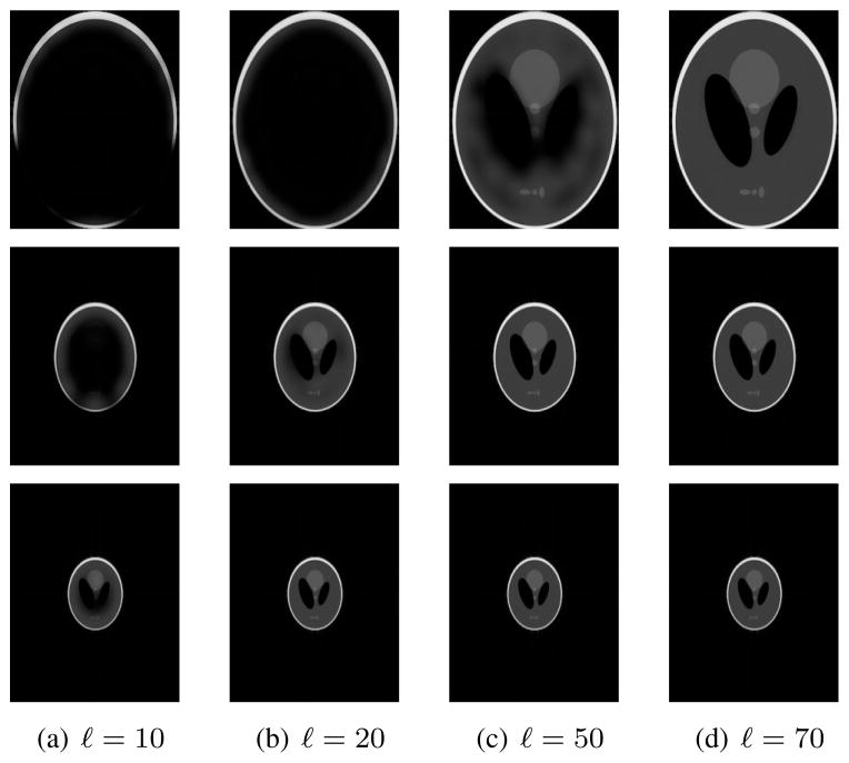
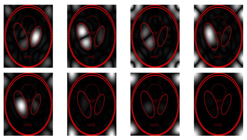
Images reconstructed after this low-rank approximation are shown in Fig. 4. The figure shows that accurate images are obtained for values of ℓ that can be substantially less than NR, with the best low-rank approximations obtained when Ωρ is small. However, reasonable low-rank approximations can still be obtained when Δk = 1, due to the fact that the image is still approximately zero within the corners of the FOV and within two relatively large ellipses near the center of the FOV. Fourier transform reconstructions f (x, y) of the 8 linearly independent nullspace vectors f̃ for which Ĉ74f̃ = 0 when R = 5 and Δk = 1 are shown in Fig. 5. Note that all of these functions are observed to have Ωf approximately disjoint from Ωρ, as expected, verifying further that C contains substantial information about the spatial support of the image.
Fig. 4.
Images generated after rank-ℓ approximation of C with R = 5. (top row) Δk = 1. (middle row) Δk = 1/2. (bottom row) Δk = 1/3.
Fig. 5.
Magnitudes of the Fourier transform reconstructions of the 8 linearly independent nullspace vectors f̃ for which Ĉ74f̃ = 0, corresponding to the images displayed in the top row of Fig. 4 with R = 5 and Δk = 1. Image edge locations are superimposed in red for visual reference.
D. Phase Constraints
We demonstrated in the previous subsections that images with limited spatial support can be associated with approximately low-rank matrices, with the matrix rows formed with data from local k-space neighborhoods. In this subsection, we demonstrate that images with slowly varying phase can be associated with similarly constructed low-rank matrices. To begin, it is useful to decompose the image into its magnitude m(x, y) = |ρ(x, y)| and phase ϕ(x, y) = ∠ρ(x, y), such that
| (7) |
where * denotes complex conjugation and h (x, y) is any function satisfying
| (8) |
It is useful to note that:
| (9) |
Based on the conjugation property of the Fourier transform, we know that the Nyquist-sampled Fourier transform of ρ*(x, y) will equal ρ̃* [−nx, −ny]. As a result, applying the convolution theorem of the Fourier transform to (9) leads to:
| (10) |
where g̃[p, q] is the Nyquist-sampled Fourier transform of (h (x, y))2. This relationship allows one side of k-space to be linearly predicted from k-space samples on the opposite side, and is used in classical half-Fourier methods [19]–[21].
If we further assume that ρ(x, y) has slowly varying phase, then (h (x, y))2 can be accurately approximated through truncation of its Fourier transform. Similar to the case of support-limited images, assuming a Fourier truncation radius of R allows us to write (10) as the pair of relationships:
| (11) |
and
| (12) |
for ∀(nx, ny) ∈ ℤ2, where subscripts r and i are used to denote the real and imaginary components of complex numbers (i.e., ρ̃r [nx, ny] and ρ̃i [nx, ny] are real-valued, with ρ̃[nx, ny] = ρ̃r [nx, ny] + iρ̃i [nx, ny]).
A novel alternative set of linear dependence relationships can be derived based on the observation that
| (13) |
where v and w are arbitrary integers.
Applying the convolution and shift theorems of the Fourier transform to (13) leads to
| (14) |
for ∀(nx, ny) ∈ ℤ2 and ∀(v, w) ∈ ℤ2, where s̃[p, q] is the Nyquist-sampled Fourier transform of h (x, y). To the best of our knowledge, no previous phase-constrained MRI reconstruction methods have used relationships of this form.
Assuming that h (x, y) exp (−i2πΔk [xv + yw]) and h* (x, y) exp (i2πΔk [xv + yw]) are both smooth functions for some value of (v, w) (i.e., making simultaneous radius-R Fourier approximations of s̃[p + v, q + w] and s̃[p − v, q − w]) leads to the pair of relationships:
| (15) |
and
| (16) |
for ∀(nx, ny) ∈ ℤ2.
E. Low-Rank Matrices and Smooth Image Phase
Similar to the case of limited image support, relations of the form shown in (11), (12), (15), and (16) enable the construction of approximately low-rank matrices. In particular, if we choose K-distinct k-space points indexed by with K ≥ NR + 1, then (11) and (12) imply that the matrix G ∈ ℝ2K×2NR+1 defined by
| (17) |
will be approximately low-rank, where vectors gr, gi ∈ ℝK and matrices Gr, Gi ∈ ℝK×NR have elements:
| (18) |
| (19) |
| (20) |
| (21) |
for k = 1, …, K and m = 1, …, NR.
Based on (11) and (12), it is expected that G would approximately nullify vectors proportional to
where g̃[p, q] is the Fourier transform of any valid (h (x, y))2 satisfying (8). However, based on (8), we would not necessarily expect there to be more than one valid (h (x, y))2 unless ρ(x, y) also has limited support. As a result, G would be rank deficient but might not have very low rank.
Alternatively, if we choose K-distinct k-space points indexed by with K ≥ NR, then (15) and (16) imply that the matrix S ∈ ℝ2K×2NR defined by
| (22) |
will be approximately rank-deficient, where matrices Sr+, Sr−, Si+, Si− ∈ ℝK×NR respectively have elements:
| (23) |
| (24) |
| (25) |
| (26) |
for k = 1, …, K and m = 1, …, NR. In addition, S potentially has a larger nullspace than G, since we could obtain valid nullspace vectors from each (v, w) combination for which radius-R approximations of s̃[p + v, q + w] and s̃[p − v, q − w] are valid. Specifically, if the image has smooth phase, then s̃[p, q] will be accurately approximated by radius-R truncation for a relatively small R. This case corresponds to (v, w) = (0, 0). Other values of (v, w) would then also be valid if R is even larger than this.
Note that, like C, each row of the G and S matrices collects k-space points from neighborhoods of radius R. However, unlike C, the points are taken from both sides of k-space.
We denote the linear3 operators that map a length-S vector of k-space samples into the matrices G and S by
 (·) :
(·) :
 → ℝ2K×2NR+1 and
 (·) :
(·) :
 → ℝ2K×2NR, respectively. Both operators are structured such that
and
are representable as S × S diagonal matrices.
F. Empirical Validation of the Characteristics of G and S
Similar to the case of C, we performed simple simulations involving the Shepp-Logan phantom to validate and evaluate the rank-characteristics of G and S. In particular, we took the magnitude image obtained when Δk = 1 (shown in Fig. 1(a)), and applied randomly generated phase profiles obtained through Fourier truncation and amplitude normalization of complex white Gaussian noise (truncation radii of Γ = 0, 1, 2, 3, 5, 10, and 20, in units of Nyquist sampling intervals).4 These phase profiles range from slowly varying to quickly varying, as illustrated in Fig. 6.
Fig. 6.

Phase profiles generated with different k-space truncation radii Γ, which are used in simulations evaluating the rank characteristics of G and S. The gray scale ranges from a phase of −π (black) to π (white).
For these simulations, we chose K = (256−2R)2 for G and K = (255−2R)2 for S, which were the maximum numbers of k-space points that had their entire neighborhood inside the 256×256 sampling grid. As before, we considered the four different neighborhood systems ΛR shown in Fig. 2.
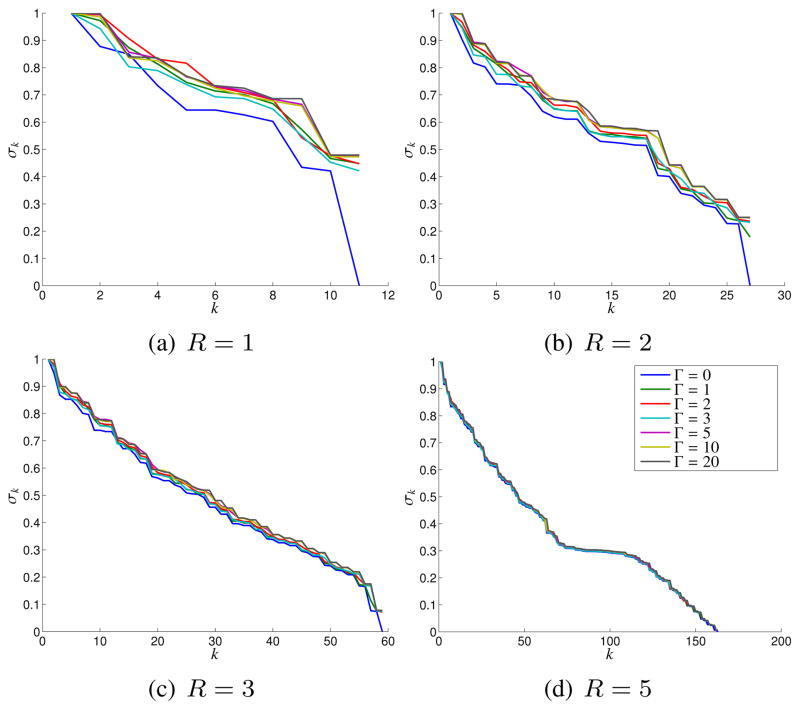
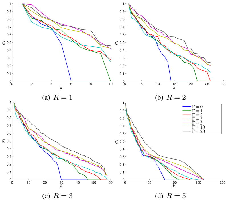
Figures 7 and 8 show plots of the singular values obtained for G and S, respectively. Figure 7 indicates that G is rank deficient when the image phase is constant (i.e., Γ = 0). However, the singular value spectrum of G is not heavily dependent on the smoothness of the image phase, and the matrix is not approximately low-rank for non-zero values of Γ unless R is large. These observations agree with our previous theoretical predictions. In particular, we might only expect a single nullspace vector since the construction of G only involved a single known linear dependence relationship. In addition, we would expect the need for large R because (h (x, y))2 will usually have more high-frequency components than h (x, y), and equivalently, because g̃[p, q] equals the convolution of s̃[p, q] with itself.
Fig. 7.
Effects of the Fourier-domain phase truncation radius Γ on the singular value spectrum of the G matrix for different neighborhood sizes R.
Fig. 8.
Effects of the Fourier-domain phase truncation radius Γ on the singular value spectrum of the S matrix for different neighborhood sizes R.
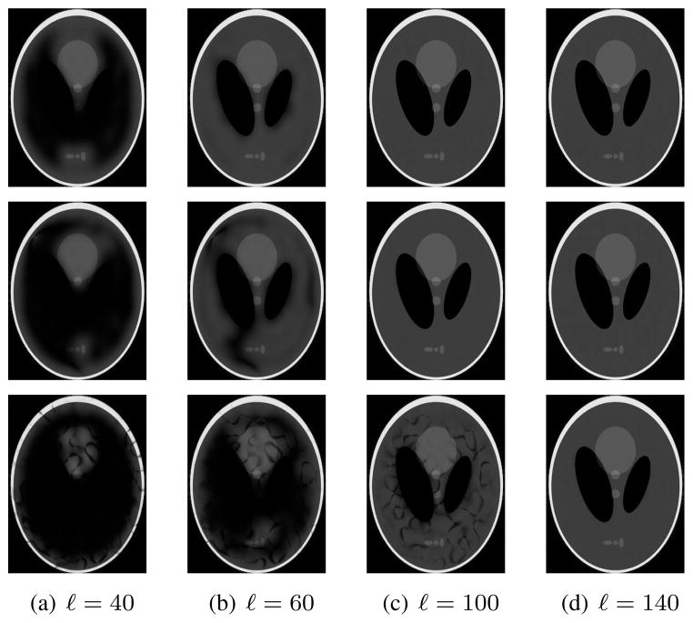
In contrast to Fig. 7, Fig. 8 shows that S can be accurately approximated as a low-rank matrix, with the effective numerical rank of the matrix decreasing as the image phase becomes smoother. Figure 9 shows images reconstructed after performing rank-ℓ approximations of S, with k-space points estimated from this matrix using MNLS estimation as described previously. As expected, accurate images are obtained for values of ℓ that can be substantially less than 2NR, with the best low-rank approximations obtained when Γ is small. We also computed similar images when performing low-rank approximations of G. As would be expected from the singular value spectra, these reconstructions were not very accurate when ℓ was much smaller than NR, and demonstrated characteristics similar to those shown in the top row of Fig. 4.5
Fig. 9.
Images generated after rank-ℓ approximation of the matrix S with R = 5. (top row) Γ = 0. (middle row) Γ = 2. (bottom row) Γ = 10.
III. Problem Formulation and Algorithm
A. Problem Formulation
Section II demonstrated theoretically and empirically that k-space data from MR images with limited support or slowly varying phase could be used to construct low-rank matrices. The practical value of low-rank modeling is that a real-valued M × N matrix with rank-L will have MN entries, but only L (M + N − L) degrees of freedom, which is much smaller number than MN when L ≪ min (M, N). As a result, it is possible to reconstruct low-rank matrices from noisy and/or highly undersampled data. There have been several different previous approaches to using rank constraints to guide data acquisition and image reconstruction in medical imaging, many of which are reviewed in [2], [25], [29].
Let k ∈
 denote the ideal vector of Nyquist-sampled noiseless k-space data, and assume we make undersampled and/or noisy measurements according to
| (27) |
where d ∈
 is the vector of noisy measured data, n ∈
 is the unknown noise, and F ∈
 is a subsampling operator which is formed by keeping M rows from the S×S identity matrix.6 In this work, we will focus specifically on low-rank matrix reconstruction problems that are posed as:
| (28) |
where is a standard least-squares functional (which corresponds to the maximum likelihood cost functional for white Gaussian noise) that is used to encourage consistency of k with the measured data, JC (·), JG (·), and JS (·) are regularizing penalty functionals that are used to encourage the matrices C, G, and S to have low-rank or rank-deficient structure, and λC, λG, and λS are scalar regularization parameters.
The choice of JC (·), JG (·), and JS (·) will determine how matrix rank constraints are incorporated into image reconstruction, and a variety of different penalty functionals have been previously proposed. Obvious choices to encourage low-rank matrix structure would be functionals of the form
| (29) |
| (30) |
where r is a user-defined parameter. Both of these functionals will encourage matrices that are strictly low rank. While the optimization problems that result from the use of these functionals are nonconvex and NP-hard to solve in general [22], there exist fast greedy algorithms for addressing problems involving these functionals that perform very well in practice and can easily incorporate additional constraints. Examples include incremented rank PowerFactorization (IRPF) [54] (which can have theoretical performance guarantees [55], and has been previously used in MRI [2], [25], [26], [29], [39]), and variations on the Cadzow algorithm [56] (also previously used in MRI [4], [37], [46], [47]).
While (29) or (30) could potentially be used for each of the three regularization functionals, it is difficult to find nontrivial vectors k such that matrices
 (k),
(k),
 (k), and
 (k) all simultaneously have exactly low-rank structure. As a result, other choices are more appealing when using (28).
Another popular choice for encouraging low-rank matrix structure is the Schatten p-norm [27], [48], given by
| (31) |
where the σk are the singular values of the matrix X. When p = 1, the Schatten p-norm is called the nuclear norm. The nuclear norm is the tightest possible convex relaxation of the functional in (29), and has theoretical performance guarantees in certain situations [22]. The nuclear norm has also been widely used in various low-rank MRI scenarios [27], [28], [30], [31], [38], and its main advantage is that the resulting optimization problems are convex and can be solved globally and efficiently from any initialization. The Schatten p-norm is nonconvex for 0 < p < 1. Despite nonconvexity, both IRPF and Schatten p-norm (with p < 1) problem formulations are observed to outperform nuclear norm formulations in a wide range of applications [2], [27], [32], [48], [54], [57].
In this work, we will consider the novel cost functional that blends elements of (30) and (31):
| (32) |
where r is a user-defined parameter and ||·||F denotes the Frobenius norm. Like (30), Eq. (32) can use prior knowledge of r to avoid penalizing matrices with rank ≤ r. Like (31), Eq. (32) also does not preclude matrices with larger ranks.
B. Algorithm
A variety of different formulations have been proposed to solve low-rank matrix reconstruction problems, and appropriate algorithms for these existing methods can be found in the previously cited references. In this subsection, we focus on a new algorithm to solve problems involving (32), which, to the best of our knowledge, have not been previously considered.
Using penalties of the form in (32) with (28) leads to
| (33) |
where we have introduced rC, rG, and rS to respectively denote the rank constraints for C, G, and S, and, without loss of generality, have used the same K and NR values for all matrices. Equation (33) is nonconvex, and we solve it using an iterative majorize-minimize (MM) approach that guarantees that the sequence of estimates k̂(i) monotonically decrease the cost function [58]. Specifically, we majorize (32) at each iteration by holding T constant at its optimal value computed for k̂(i−1). See [58] for further details of MM methods. Pseudocode for the algorithm is given in Alg. 1.
Algorithm 1.
| ||
|
The low-rank approximation problems in steps 2(a–c) of Alg. 1 are solved using the truncated SVD. The linear least-squares problem (34) is solved easily using
| (35) |
where Φ† is the pseudoinverse of the matrix
| (36) |
This pseudoinverse-based solution is particularly simple to compute, due to the fact that Φ is a diagonal matrix.
The SVD calculations are the most time consuming aspect of Alg. 1, though it should be noted that fast algorithms for this problem are in active development by a number of groups. For simplicity, our truncated SVD computations used the older PROPACK [59] MATLAB toolbox. Typical SVD computation times for the experiments shown in the next section were 5–10 seconds per SVD. As a result, our relatively unoptimized MATLAB implementation of Alg. 1 typically took ten minutes or more to converge. Substantial speed increases would be possible if using more optimized software.
The choice of k̂(0) could be important, since the cost function is nonconvex and the iterations might converge to a local minimum. In all of our results, we simply set k̂(0) equal to the zero-filled original k-space data, though other choices could yield even better outcomes.
IV. Results
The practical value of constrained reconstruction methods is always context-dependent, and requires extensive application-specific evaluation. This kind of assessment is beyond the scope of this paper and is left to future work. Instead, the objective of this section is to demonstrate the potential of LORAKS in a variety of settings and to compare with other commonly-used constraints.
A. Denoising Example
Our first example illustrates the potential of using LORAKS to reduce noise in fully sampled data. Nyquist-sampled high-SNR data (512×256 sampling grid corresponding to a 60 mm × 30 mm FOV) was acquired from a section of kiwi fruit using a 2D spin-echo pulse sequence (TE=30 ms, TR=6000 ms, 1 mm slice thickness) on a 14.1 T scanner. This image was used as a gold standard, and pseudorandom complex white Gaussian noise was added to simulate a lower-SNR acquisition (the average image intensity was a little more than 2× larger than the standard deviation of the simulated noise in the reconstructed image). Reconstructions were performed using LORAKS with R = 5 and a range of different rC, rG, and rS values. The regularization parameters were chosen as λC = 1010/NC, λG = 1010/NG, and λS = 1010/NS, where NC, NG, and NS, are respectively the number of entries in the matrices C, G, and S. The use of large regularization parameters ensures that the rank constraints will be imposed much more strongly than the data consistency constraint, which is desirable when using LORAKS to reduce noise.
Representative LORAKS results are shown in Fig. 10(a–d), where the rC, rG, and rS parameters were chosen to minimize the normalized ℓ2-norm reconstruction error. As can be seen, LORAKS reconstruction has substantially reduced the amount of noise. This is most visually obvious outside of the image support, where the noise has been almost completely suppressed. However, noise has also been reduced within the support of the image, though to a lesser extent. This fact is more evident in the mean-squared error images shown in Fig. 10(e,f) (generated based on reconstructing the kiwi data 100 times with different simulated noise realizations), which demonstrate error reductions throughout the FOV. However, it should also be noted that there are some image regions where true image structure has also been suppressed or attenuated to some extent, and this tends to occur in regions where the original image intensity was low (e.g., the center of the image and the edges of the image support). As with most model-based reconstruction/denoising methods, this problem can be mitigated by imposing the model less aggressively, at the cost of less-effective noise suppression. Finally, we note that the ℓ2-norm error metric, which we used to select the LORAKS parameters in this example, has the limitation that images with small ℓ2-norm errors are frequently not the most visually pleasing or perceptually faithful images [60]. The optimal choice of error metrics and LORAKS parameters will, in general, be application dependent.
Fig. 10.
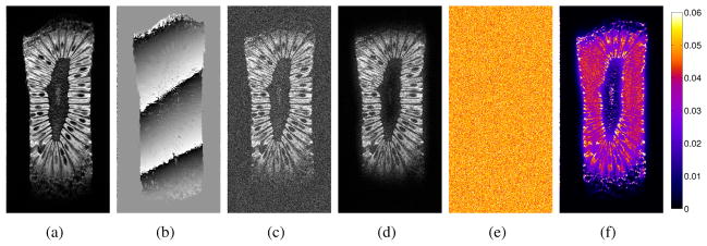
LORAKS denoising of the kiwi fruit dataset. (a) High-SNR magnitude image. (b) High-SNR phase image. (c) Magnitude image generated from the low-SNR simulation with conventional Fourier reconstruction. (d) LORAKS reconstruction using rC = 31, rG = 21, and rS = 70. Also shown are mean-squared error images corresponding to (e) conventional Fourier reconstruction and (f) LORAKS reconstruction with rC = 31, rG = 21, and rS = 70. The colorscale has been normalized such that the grayscale ranges from 0 to 1 for the images in (a–d).
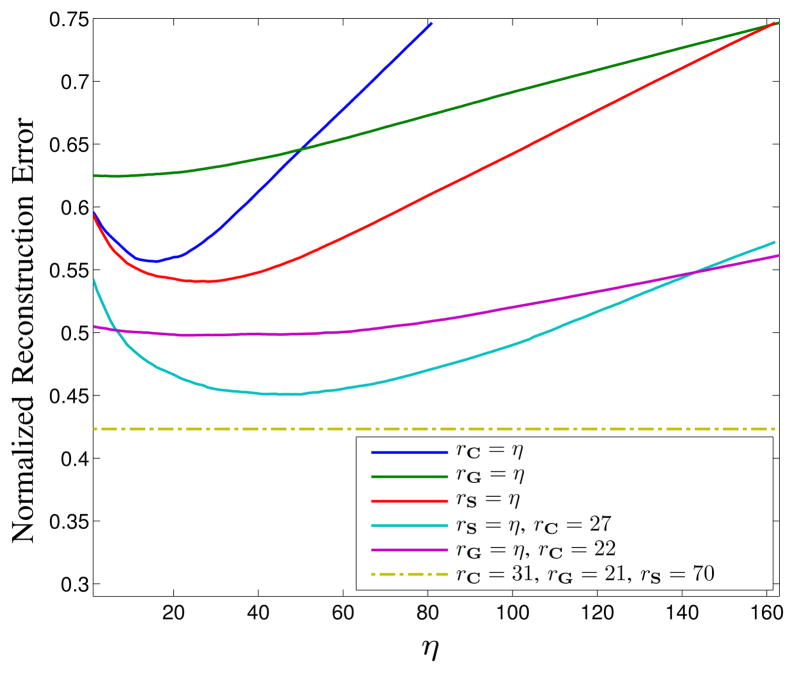
Figure 11 illustrates the quantitative effects of different choices of rC, rG, and rS on the LORAKS reconstruction. We observe that each of the different low-rank matrices C, G, and S can independently improve the reconstruction error when rC, rG, and rS are chosen properly. We also observe that the use of the S-based constraint leads to the most significant improvements, followed by the use of C-based constraints. The G-based constraints are the least effective in this example. However, it should be noted that the joint use of C-, G-, and S-based constraints leads to substantially better denoising performance than is achieved using any of these constraints individually, and that for best performance, the choices of rC, rG, and rS should not be made independently.
Fig. 11.
Plots of normalized ℓ2-norm reconstruction error as a function of the rank constraint parameters rC, rG, and rS. When particular rank constraint values are not given for specific curves, it indicates that the corresponding rank constraints were not imposed. Note that when G-based constraints are not used, the LORAKS reconstruction achieves its optimal value when rC=27 (cyan curve). When S-based constraints are not used, the LORAKS reconstruction achieves its optimal value when rC=22 (purple curve). When all constraints are used, the LORAKS reconstruction achieves its optimal value when rC=31, rG=21, and rS=70 (dark yellow dash-dotted curve).
B. Sparse Sampling Examples
The LORAKS framework was also applied to reconstruct sparsely sampled k-space data from two different human brain datasets, as shown in Figs. 12–14 and described below.
Fig. 12.
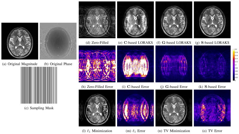
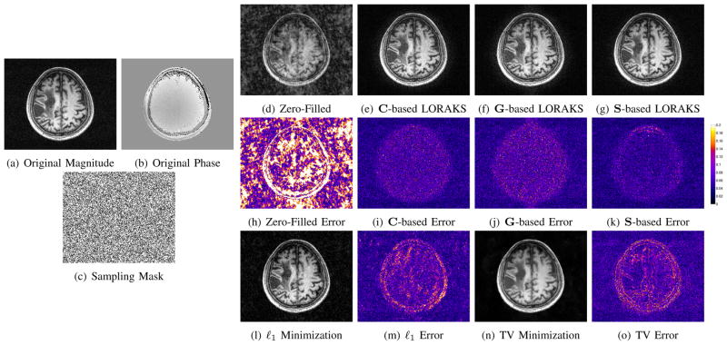
LORAKS reconstruction of an undersampled T2-weighted spin-echo brain image of a healthy subject. (a) Magnitude of the fully sampled reference image. (b) Phase of the fully sampled reference image. (c) Random k-space sampling mask. (d) Zero-filled Fourier reconstruction. (e) LORAKS reconstruction with rC = 50. (f) LORAKS reconstruction with rG = 120. (g) LORAKS reconstruction with rS = 70. Note that the reconstructions shown in (f) and (g) still contain small residual aliasing artifacts, which are visible upon close inspection. (h–k) Error images corresponding to the reconstructions shown in (d–g). The colorscale has been normalized such that the grayscale ranges from 0 to 1 for the images in (d–g). For comparison, ℓ1-norm and TV minimization results are shown in (l) and (n), respectively, with corresponding error images shown in (m) and (o).
Fig. 14.
LORAKS reconstruction of an undersampled T1-weighted MPRAGE brain image of a patient with a stroke lesion. (a) Magnitude of the fully sampled reference image. (b) Phase of the fully sampled reference image. (c) Random sampling mask. (d) Zero-filled Fourier reconstruction. (e) LORAKS reconstruction with rC = 50. (f) LORAKS reconstruction with rG = 105. (g) LORAKS reconstruction with rS = 75. (h–k) Error images corresponding to the reconstructions shown in (d–g). The colorscale has been normalized such that the grayscale ranges from 0 to 1 for the images in (d–g). For comparison, ℓ1-norm and TV minimization results are shown in (l) and (n), respectively, with corresponding error images shown in (m) and (o).
1) T2-Weighted Image
Figure 12 shows an example where data was obtained by retrospectively subsampling lines of k-space from a T2-weighted axial brain image of a healthy subject. The fully sampled reference image (256×256 Nyquist sampling grid corresponding to a 210 mm × 210 mm FOV) was acquired using a 2D multislice turbo spin-echo sequence (TE=88 ms, TR=10000 ms, 3 mm slice thickness) on a 3T scanner with a 12-channel head coil. To assess LORAKS on single-channel data, the 12-channel data was compressed to a single virtual coil using the SVD [61], [62]. Since the data was acquired with a standard human research protocol and had a typical amount of experimental noise, no additional simulated noise was included. Subsampling was designed so that 160 lines of k-space were acquired (5/8ths of the fully sampled data), with a random distribution of phase encoding locations. The sampling scheme included the central line of k-space, but as seen from the sampling mask shown in Fig. 12(c), there is no fully sampled calibration region that could be used to estimate image phase or support in the conventional manner.
For simplicity, LORAKS reconstructions were performed using C-, G-, and S-based constraints independently, with the rC, rG, and rS parameters chosen subjectively based on visual image quality. Unlike the previous denoising example, regularization parameters were chosen to emphasize data fidelity (λC = 10−10/NC, λG = 10−10/NG, and λS = 10−10/NS). This has the effect of preserving high-SNR measured data, and only using the rank constraints to extrapolate missing data.
As Fig. 12(a–k) illustrates, the different rank constraints are each able to enhance reconstruction, but have different characteristics. In this case, C-based constraints are able to reduce aliasing artifacts outside the support of the true image, though substantial artifacts still remain within the support of the image. Both G- and S-based constraints are able to substantially reduce aliasing artifacts throughout the FOV. As in the case of denoising, S-based constraints again appear to be more powerful than the other constraints. For this example, the use of joint constraints involving C, G, and S only leads to moderate improvements over using S-based constraints alone.
To further illustrate the flexibility and generality of LORAKS, Fig. 13 presents another example based on this dataset where we have replaced random k-space sampling with the more conventional “half k-space” sampling scheme that is commonly used with calibration-based phase-constrained reconstruction methods. Rather than sampling exactly half of k-space, we used the typical 5/8ths partial Fourier acquisition that acquires extra calibration lines at the center of k-space. These lines are used to estimate image phase in conventional calibration-based methods, while LORAKS treats these lines exactly the same as it treats any other k-space lines.
Fig. 13.
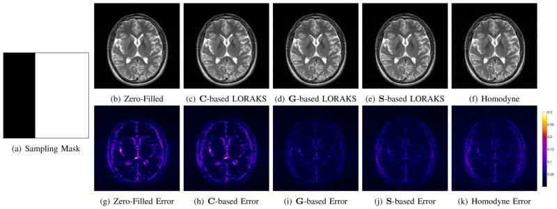
LORAKS reconstruction of the image from Fig. 12 with a “half k-space” sampling pattern. (a) Sampling mask. (b) Zero-filled Fourier reconstruction. (c) LORAKS reconstruction with rC = 50. (d) LORAKS reconstruction with rG = 120. (e) LORAKS reconstruction with rS = 70. (f) Homodyne reconstruction [20]. Note that close inspection might be necessary to visualize the differences between the images shown in (b–f). (g–k) Error images corresponding to the reconstructions shown in (b–f). The colorscale has been normalized such that the grayscale ranges from 0 to 1 for the images in (b–f).
As demonstrated in the figure, the phase-based LORAKS constraints (i.e., constraints based on G and S) are both effective in reducing the undersampling artifacts and restoring image resolution. On the other hand, the C-based constraint is ineffective in this case. This is not surprising, since this kind of k-space sampling scheme is designed for use with phase constraints. Notably, the figure also shows that the phase-based LORAKS reconstructions perform similar to (if not slightly better than) the commonly used homodyne method [20] (a calibration-based phase-constrained reconstruction method).
2) T1-Weighted Image
Figure 14 shows an example where data was obtained by retrospectively subsampling lines of k-space from a T1-weighted brain image of a patient with a stroke lesion. The fully sampled reference image (1 mm3 isotropic resolution with a 256×256×208 Nyquist sampling grid) was acquired using a 3D MPRAGE sequence (TE=3 ms, TR=2500 ms, TI=800 ms, 10° flip angle) on a 3T scanner. As before, data was acquired with a 12-channel head coil which was compressed to a single virtual channel, and no simulated noise was added to the data. Inverse Fourier transformation was performed along the fully sampled frequency encoding dimension (superior-inferior), to enable independent reconstruction of 2D slice images. Subsampling was designed so that 33280 lines of k-space were acquired (5/8ths of the fully sampled data), with a random distribution of phase encoding locations. Compared to the 2D acquisition considered in the previous case, the 3D acquisition enables Fourier subsampling with more incoherent aliasing artifacts [44]. As in the previous example, the sampling scheme includes the center of k-space, but there is no fully sampled calibration region. LORAKS reconstructions were performed independently with C-, G-, and S-based constraints, with regularization parameters chosen small (λC = 10−10/NC, λG = 10−10/NG, and λS = 10−10/NS) to emphasize data consistency.
The results in Fig. 14(a–k) again show that the LORAKS framework is capable of reconstructing undersampled data. Similar to the previous randomly undersampled experiment, we observe that the S-based constraint yielded the best results, with only moderate improvements in image quality from jointly using C-, G-, and S-based constraints.
C. Comparisons
LORAKS is possible because of support and/or phase assumptions, and it is worth noting that other regularized MR image reconstruction methods have been proposed that make use of similar constraints in a more direct way. In particular, an image with limited support is sparse in the spatial domain. As a result, it might be reasonable to try reconstructing support-limited images using alternative sparsity-promoting regularized reconstruction methods like ℓ1-norm minimization [44]. Similarly, it might be reasonable to directly regularize the image phase if assuming phase varies slowly [45].
To explore this issue, the undersampled datasets from Figs. 12 and 14 were also reconstructed using two sparsity-based reconstruction methods. Specifically, images were reconstructed using sparsity-based support constraints (via ℓ1-norm minimization [44] in the canonical basis) and sparsity-based image smoothness constraints (via total variation (TV) minimization [44]).7 In all cases, optimization was performed using the version of Nesterov’s algorithm described in [63], and regularization parameters were optimized manually to achieve the smallest possible reconstruction errors (using the ℓ2-norm error metric). Reconstructions are shown in Figs. 12(l–o) and 14(l–o). It is clear from these reconstructions that LORAKS constraints provide information that is distinct from the information provided by the other constraints. In particular, the ℓ1-norm and TV reconstructions have substantially larger error than the best of the LORAKS reconstructions for each dataset, and the spatial structure of the error is quite different for the ℓ1-norm and TV reconstructions than for the LORAKS reconstructions.
The reconstructed image shown in Fig. 12(l) is particularly interesting, because it is “sparser” (i.e., has smaller ℓ1-norm) than the fully-sampled image or any of the LORAKS reconstructions. In this case, the actual image support has been misidentified by ℓ1-norm minimization, and many of the voxels inside the brain erroneously have negligible intensities. In contrast, all three LORAKS reconstructions reconstruct the image support more accurately.8 One reason for this difference is that LORAKS assumes slightly more about image sparsity than ℓ1-norm minimization does. Specifically, the use of the ΛR neighborhood system with relatively small R means that LORAKS only prefers spatial sparsity if the voxels where ρ(x, y) = 0 are spatially clustered together. In contrast, ℓ1-minimization is indifferent to the the spatial distribution of the voxels where ρ(x, y) = 0, which in this case, has lead to a reconstruction with unrealistic holes in the image support. Another reason for the difference between LORAKS and the other methods might be that uniform random k-space sampling is often suboptimal for ℓ1-norm and TV minimization – sparsity-based reconstructions are generally much better when using variable density sampling [44], [63].
V. Discussion and Conclusions
This work demonstrated that images with limited spatial support and/or smoothly varying phase can be mapped into low-rank matrices because of consistent linear dependencies within local k-space neighborhoods. Based on this, we proposed the LORAKS framework for constrained image reconstruction, which imposes phase- and support-constraints implicitly through low-rank matrix modeling. In addition, we described an example implementation of LORAKS that introduced a novel regularization penalty and a corresponding new algorithm for promoting low-rank matrix structure.
As mentioned above, theoretical performance guarantees exist for existing low-rank matrix recovery methods under certain conditions on the matrix and the sampling scheme [22], [55]. As a result, we might also expect that theoretical guarantees could potentially be derived for LORAKS. This kind of exploration is beyond the scope of this paper, but is a promising direction for future research.
While the use of phase- and support-constraints is classical in constrained MRI, our results indicate that the LORAKS framework is considerably more flexible than previous calibration-based approaches, and demonstrates good image reconstruction performance in a variety of different settings. In particular, we demonstrated the ability to use LORAKS to denoise low-SNR data, to reconstruct undersampled data acquired with conventional “half k-space” sampling schemes, and to reconstruct undersampled data acquired with calibrationless random-sampling schemes.
Since LORAKS is based on a regularized formulation of image reconstruction, it is easy to include additional regularization penalties, such as the smoothness, sparsity, and rank penalties that are frequently used for constrained imaging in a variety of different application settings [2]. Indeed, we recommend the use of LORAKS with additional constraints, since the constraints imposed by LORAKS are potentially complementary to existing constrained imaging approaches.
Like many other regularization-based methods, the performance of LORAKS depends on the choice of various parameters which influence the tradeoff between the ill-posedness of the inverse problem (which is more severe if the problem is under-constrained) and the reconstruction bias introduced by the image model (which is more severe if the problem is over-constrained). Our cost function in Eq. (33) required the choice of several parameters: λC, λG, λS, rC, rS, rG, K, and R. We chose these manually in our implementations, though observed that our results were not highly sensitive to small variations in our choices. The choice of parameters is also substantially simplified when using only one LORAKS constraint (as in Figs. 12–14) instead of all three. Automatic selection of these parameters is an interesting topic for future work.
In addition to reconstruction parameters, the performance of LORAKS is also dependent on image structure. Specifically, LORAKS assumes that the C, G, and S matrices all have relatively low rank. In cases where the support is not small and/or the phase varies rapidly, the matrix rank will not be as low and LORAKS constraints will be weaker.
For simplicity, our description of low-rank structure in k-space focused on 2D imaging. However, 3D imaging is also fully compatible with the LORAKS framework, and generalizations to spatiotemporal imaging are also straightforward. In particular, spatiotemporal MR images generally have very sparse support in the x-f domain [14]–[16], [27], [31], [32], [57] and also frequently have slow phase variation along the temporal dimension. As a result, low-rank matrices could easily be constructed within the LORAKS framework from samples in local k-t and/or k-f neighborhoods.
Finally, the LORAKS framework is also easily extended to parallel imaging scenarios. In particular, we should note that the previously proposed SAKÉ method [34] is highly related to our proposed C-based LORAKS approach, despite being derived in a completely different way. The two approaches are actually equivalent (neglecting minor differences in ΛR) if SAKÉ is applied to single-channel data instead of the multi-channel data it was designed for. Noting that C-based constraints were generally less powerful than S-based constraints in our evaluation of LORAKS, we expect that the generalization of S-based constraints to parallel imaging scenarios could yield additional major benefits.
Acknowledgments
This work was supported in part by research grant NIH-R01-NS074980.
Footnotes
This toy example was designed to show proof-of-principle evidence that limited image support implies that the C matrix has low rank. The images obtained using very small Δk are not intended to represent realistic MRI experiments (which will generally have FOVs that are chosen reasonably well). However, images with very small spatial support (similar to the small Δk images from this example) can occur in parallel imaging contexts if the coil sensitivity profiles have limited spatial support [51], and in dynamic imaging contexts (after subtracting a baseline image) if the time-varying components of the image are localized to a small region of the FOV [52].
The requirement that K ≥ NR will generally place limits on the maximum value of R. This is because the maximum value of K will generally decrease as R increases, due to the fact that there will be fewer points whose entire neighborhood system fits within the Nyquist-sampled k-space grid.
These operators are not actually linear with respect to complex vectors in
 , but are linear with respect to an equivalent representation that concatenates the real and imaginary parts into a real vector in ℝ2S. We will neglect this nuance to ease notation.
Amplitude normalization implies that the phase functions h*(x, y) generated in this way will not be exactly bandlimited to radius-Γ in the Fourier domain, despite the fact that Fourier truncation was used to generate them.
It is not surprising that low-rank approximations of G and C have similar characteristics, since they are constructed from similar neighborhood systems.
Our choice of F restricts us to Cartesian sampling patterns. Similar to previous work [35], non-Cartesian extensions are easy to derive.
We did not directly compare against [45], because the optimization problem described in [45] is nonconvex, and is quite sensitive to local minima if the algorithm is not initialized well. As a result, [45] assumes that calibration data is available to provide an accurate initial phase estimate. This assumption is not compatible with our calibrationless sampling schemes. Instead, we compared against the convex TV constraint, which encourages smoothness of both the image magnitude and phase (instead of just the phase).
It is worth noting that while C-based LORAKS (the LORAKS approach that uses assumptions that are most similar to those of ℓ1-minimization) accurately identifies the image support, the reconstruction quality is still relatively poor. This is not surprising because the support of the object is relatively large, while the undersampling is considerable.
Personal Use of this material is permitted. However, permission to use this material for any other purposes must be obtained from the IEEE by sending a request to pubs-permissions@ieee.org.
References
- 1.Liang ZP, Boada F, Constable T, Haacke EM, Lauterbur PC, Smith MR. Constrained reconstruction methods in MR imaging. Rev Magn Reson Med. 1992;4:67–185. [Google Scholar]
- 2.Haldar JP. PhD dissertation. University of Illinois; Urbana-Champaign, Urbana, IL, USA: 2011. Constrained imaging: Denoising and sparse sampling. [Online]. Available: http://hdl.handle.net/2142/24286. [Google Scholar]
- 3.Griswold MA, Jakob PM, Heidemann RM, Nittka M, Jellus V, Wang J, Kiefer B, Haase A. Generalized autocalibrating partially parallel acquisitions (GRAPPA) Magn Reson Med. 2002;47:1202–1210. doi: 10.1002/mrm.10171. [DOI] [PubMed] [Google Scholar]
- 4.Lustig M, Pauly JM. SPIRiT: Iterative self-consistent parallel imaging reconstruction from arbitary k-space. Magn Reson Med. 2010;65:457–471. doi: 10.1002/mrm.22428. [DOI] [PMC free article] [PubMed] [Google Scholar]
- 5.Zhang J, Liu C, Moseley ME. Parallel reconstruction using null operations. Magn Reson Med. 2011;66:1241–1253. doi: 10.1002/mrm.22899. [DOI] [PMC free article] [PubMed] [Google Scholar]
- 6.Smith MR, Nichols ST, Henkelman RM, Wood ML. Application of autoregressive moving average parametric modeling in magnetic resonance image reconstruction. IEEE Trans Med Imag. 1986;MI–5:132–139. doi: 10.1109/TMI.1986.4307762. [DOI] [PubMed] [Google Scholar]
- 7.Barone P, Sebastiani G. A new method of magnetic resonance image reconstruction with short acquisition time and truncation artifact reduction. IEEE Trans Med Imag. 1992;11:250–259. doi: 10.1109/42.141649. [DOI] [PubMed] [Google Scholar]
- 8.Martin JF, Tirendi CF. Modified linear prediction modeling in magnetic resonance imaging. J Magn Reson. 1989;82:392–399. [Google Scholar]
- 9.Hess CP, Liang ZP. A data-consistent linear prediction method for image reconstruction from finite Fourier samples. Int J Imag Syst Tech. 1996;7:136–140. [Google Scholar]
- 10.Cao Y, Levin DN. Feature-recognizing MRI. Magn Reson Med. 1993;30:305–317. doi: 10.1002/mrm.1910300306. [DOI] [PubMed] [Google Scholar]
- 11.Cao Y, Levin DN. Acquisition and reconstruction of the principal components of an image: A novel MRI technique for reducing scanning time. Int J Imag Syst Tech. 1995;6:191–202. [Google Scholar]
- 12.Cheung KF, Marks RJ., II Imaging sampling below the Nyquist density without aliasing. J Opt Soc Am A. 1990;7:92–105. [Google Scholar]
- 13.Plevritis SK, Macovski A. Spectral extrapolation of spatially bounded images. IEEE Trans Med Imag. 1995;14:487–497. doi: 10.1109/42.414614. [DOI] [PubMed] [Google Scholar]
- 14.Madore B, Glover GH, Pelc NJ. Unaliasing by Fourier-encoding the overlaps using the temporal dimension (UNFOLD), applied to cardiac imaging and fMRI. Magn Reson Med. 1999;42:813–828. doi: 10.1002/(sici)1522-2594(199911)42:5<813::aid-mrm1>3.0.co;2-s. [DOI] [PubMed] [Google Scholar]
- 15.Tsao J, Boesiger P, Pruessmann KP. k-t BLAST and k-t SENSE: Dynamic MRI with high frame rate exploiting spatiotemporal correlations. Magn Reson Med. 2003;50:1031–1042. doi: 10.1002/mrm.10611. [DOI] [PubMed] [Google Scholar]
- 16.Sharif B, Derbyshire JA, Faranesh AZ, Bresler Y. Patient-adaptive reconstruction and acquisition in dynamic imaging with sensitivity encoding (PARADISE) Magn Reson Med. 2010;64:501–513. doi: 10.1002/mrm.22444. [DOI] [PMC free article] [PubMed] [Google Scholar]
- 17.Sen Gupta A, Liang Z-P. Dynamic imaging by temporal modeling with principal component analysis. Proc Int Soc Magn Reson Med. 2001:10. [Google Scholar]
- 18.Liang Z-P. Spatiotemporal imaging with partially separable functions. Proc IEEE Int Symp Biomed Imag. 2007:988–991. [Google Scholar]
- 19.Margosian P, Schmitt F, Purdy D. Faster MR imaging: imaging with half the data. Health Care Instrum. 1986;1:195–197. [Google Scholar]
- 20.Noll DC, Nishimura DG, Macovski A. Homodyne detection in magnetic resonance imaging. IEEE Trans Med Imag. 1991;10:154–163. doi: 10.1109/42.79473. [DOI] [PubMed] [Google Scholar]
- 21.Huang F, Lin W, Li Y. Partial Fourier reconstruction through data fitting and convolution in k-space. Magn Reson Med. 2009;62:1261–1269. doi: 10.1002/mrm.22128. [DOI] [PubMed] [Google Scholar]
- 22.Recht B, Fazel M, Parrilo PA. Guaranteed minimum-rank solutions of linear matrix equations via nuclear norm minimization. SIAM Rev. 2010;52:471–501. [Google Scholar]
- 23.Candès EJ, Romberg J, Tao T. Robust uncertainty principles: exact signal reconstruction from highly incomplete frequency information. IEEE Trans Inf Theory. 2006;52:489–509. [Google Scholar]
- 24.Donoho DL. Compressed sensing. IEEE Trans Inf Theory. 2006;52:1289–1306. [Google Scholar]
- 25.Haldar JP, Liang Z-P. Spatiotemporal imaging with partially separable functions: A matrix recovery approach. Proc IEEE Int Symp Biomed Imag. 2010:716–719. [Google Scholar]
- 26.Zhao B, Haldar JP, Brinegar C, Liang Z-P. Low rank matrix recovery for real-time cardiac MRI. Proc IEEE Int Symp Biomed Imag. 2010:996–999. [Google Scholar]
- 27.Lingala SG, Hu Y, DiBella E, Jacob M. Accelerated dynamic MRI exploiting sparsity and low-rank structure: k-t SLR. IEEE Trans Med Imag. 2011;30:1042–1054. doi: 10.1109/TMI.2010.2100850. [DOI] [PMC free article] [PubMed] [Google Scholar]
- 28.Trzasko J, Manduca A. Local versus global low-rank promotion in dynamic MRI series reconstruction. Proc Int Soc Magn Reson Med. 2011:4371. [Google Scholar]
- 29.Haldar JP, Liang Z-P. Low-rank approximations for dynamic imaging. Proc IEEE Int Symp Biomed Imag. 2011:1052–1055. [Google Scholar]
- 30.Gao H, Rapacchi S, Wang D, Moriarty J, Meehan C, Sayre J, Laub G, Finn P, Hu P. Compressed sensing using prior rank, intensity and sparsity model (PRISM): Applications in cardiac cine MRI. Proc Int Soc Magn Reson Med. 2012:2242. [Google Scholar]
- 31.Otazo R, Candès E, Sodickson DK. Low-rank and sparse matrix decomposition for accelerated DCE-MRI with background and contrast separation. Proc ISMRM Workshop on Data Sampling & Image Reconstruction. 2013 [Google Scholar]
- 32.Majumdar A. Improved dynamic MRI reconstruction by exploiting sparsity and rank-deficiency. Magn Reson Imag. 2013;31:789–795. doi: 10.1016/j.mri.2012.10.026. [DOI] [PubMed] [Google Scholar]
- 33.Zhang T, Alley M, Lustig M, Pauly J, Vasanawala S. Fast 3D DCE-MRI with sparsity and low-rank enhanced SPIRiT (SLR-SPIRiT) Proc ISMRM Workshop on Data Sampling & Image Reconstruction. 2013 [Google Scholar]
- 34.Lustig M, Elad M, Pauly JM. Calibrationless parallel imaging reconstruction by structured low-rank matrix completion. Proc Int Soc Magn Reson Med. 2010:2870. doi: 10.1002/mrm.24997. [DOI] [PMC free article] [PubMed] [Google Scholar]
- 35.Lustig M. Post-cartesian calibration less parallel imaging reconstruction by structured low-rank matrix completion. Proc Int Soc Magn Reson Med. 2011:483. doi: 10.1002/mrm.24997. [DOI] [PMC free article] [PubMed] [Google Scholar]
- 36.Trzasko JD, Manduca A. CLEAR: Calibration-free parallel imaging using locally low-rank encouraging reconstruction. Proc Int Soc Magn Reson Med. 2012:517. [Google Scholar]
- 37.Nguyen HM, Peng X, Do MN, Liang ZP. Denoising MR spectroscopic imaging data with low-rank approximations. IEEE Trans Biomed Eng. 2013;60:78–89. doi: 10.1109/TBME.2012.2223466. [DOI] [PMC free article] [PubMed] [Google Scholar]
- 38.Trzasko JD, Sharma SD, Manduca A. Calibrationless chemical shift encoded imaging. Proc ISMRM Workshop on Data Sampling & Image Reconstruction. 2013 [Google Scholar]
- 39.Lam F, Babacan SD, Haldar JP, Weiner MW, Schuff N, Liang Z-P. Denoising diffusion-weighted magnitude MR images using rank and edge constraints. Magn Reson Med. 2013 doi: 10.1002/mrm.24728. In Press. [DOI] [PMC free article] [PubMed] [Google Scholar]
- 40.Adluru G, Chen L, Feinberg D, Anderson J, DiBella EVR. Improving rank constrained reconstructions using prior information with reordering. Proc Int Soc Magn Reson Med. 2012:2248. [Google Scholar]
- 41.Gao H, Li L, Hu XP. Compressive diffusion MRI – part 1: Why low rank? Proc Int Soc Magn Reson Med. 2013:610. doi: 10.1002/mrm.25052. [DOI] [PMC free article] [PubMed] [Google Scholar]
- 42.Lam F, Zhao B, Liu Y, Liang Z-P. Accelerated fMRI using low-rank model and sparsity constraints. Proc Int Soc Magn Reson Med. 2013:2620. doi: 10.1002/mrm.25421. [DOI] [PMC free article] [PubMed] [Google Scholar]
- 43.Muckley MJ, Peltier SJ, Noll DC, Fessler JA. Model-based reconstruction for physiological noise correction in functional MRI. Proc Int Soc Magn Reson Med. 2013:2623. [Google Scholar]
- 44.Lustig M, Donoho D, Pauly JM. Sparse MRI: The application of compressed sensing for rapid MR imaging. Magn Reson Med. 2007;58:1182–1195. doi: 10.1002/mrm.21391. [DOI] [PubMed] [Google Scholar]
- 45.Zhao F, Noll DC, Nielsen JF, Fessler JA. Separate magnitude and phase regularization via compressed sensing. IEEE Trans Med Imag. 2012;31:1713–1723. doi: 10.1109/TMI.2012.2196707. [DOI] [PMC free article] [PubMed] [Google Scholar]
- 46.Haldar JP. Calibrationless partial Fourier reconstruction of MR images with slowly-varying phase: A rank-deficient matrix recovery approach. Proc ISMRM Workshop on Data Sampling & Image Reconstruction. 2013 [Google Scholar]
- 47.Dologlou I, van Ormondt D, Carayannis G. MRI scan time reduction through non-uniform sampling and SVD-based estimation. Signal Process. 1996;55:207–219. [Google Scholar]
- 48.Majumdar A, Ward RK. An algorithm for sparse MRI reconstruction by Schatten p-norm minimization. Magn Reson Imag. 2011;29:408–417. doi: 10.1016/j.mri.2010.09.001. [DOI] [PubMed] [Google Scholar]
- 49.Andrews HC, Patterson CL., III Singular value decomposition (SVD) image coding. IEEE Trans Comm. 1976;24:425–432. [Google Scholar]
- 50.Pan SX, Kak AC. A computational study of reconstruction algorithms for diffraction tomography: Interpolation versus filtered backpropagation. IEEE Trans Acoust, Speech, Signal Process. 1983;ASSP-31:1262–1275. [Google Scholar]
- 51.Griswold MA, Jakob PM, Nittka M, Goldfarb JW, Haase A. Partially parallel imaging with localized sensitivities (PILS) Magn Reson Med. 2000;44:602–609. doi: 10.1002/1522-2594(200010)44:4<602::aid-mrm14>3.0.co;2-5. [DOI] [PubMed] [Google Scholar]
- 52.Nagle SK, Levin DN. Multiple region MRI. Magn Reson Med. 1999;41:774–786. doi: 10.1002/(sici)1522-2594(199904)41:4<774::aid-mrm17>3.0.co;2-d. [DOI] [PubMed] [Google Scholar]
- 53.Eckart C, Young G. The approximation of one matrix by another of lower rank. Psychometrika. 1936;1:211–218. [Google Scholar]
- 54.Haldar JP, Hernando D. Rank-constrained solutions to linear matrix equations using PowerFactorization. IEEE Signal Process Lett. 2009;16:584–587. doi: 10.1109/LSP.2009.2018223. [DOI] [PMC free article] [PubMed] [Google Scholar]
- 55.Jain P, Netrapalli P, Sanghavi S. Low-rank matrix completion using alternating minimization. ACM Symp Theory Comput. 2013 [Google Scholar]
- 56.Cadzow JA. Signal enhancement – a composite property mapping algorithm. IEEE Trans Acoust, Speech, Signal Process. 1988;36:49–62. [Google Scholar]
- 57.Zhao B, Haldar JP, Christodoulou AG, Liang ZP. Image reconstruction from highly undersampled (k, t)-space data with joint partial separability and sparsity constraints. IEEE Trans Med Imag. 2012;31:1809–1820. doi: 10.1109/TMI.2012.2203921. [DOI] [PMC free article] [PubMed] [Google Scholar]
- 58.Hunter DR, Lange K. A tutorial on MM algorithms. Am Stat. 2004;58:30–37. [Google Scholar]
- 59.Larsen RM. Tech Rep DAIMI PB-357. Department of Computer Science, Aarhus University; 1998. Lanczos bidiagonalization with partial reorthogonalization. [Online]. Available: http://soi.stanford.edu/~rmunk/PROPACK/ [Google Scholar]
- 60.Wang Z, Bovik AC. Mean squared error: Love it or leave it? a new look at signal fidelity measures. IEEE Signal Process Mag. 2009;26:98–117. [Google Scholar]
- 61.Huang F, Vijayakumar S, Li Y, Hertel S, Duensing GR. A software channel compression technique for faster reconstruction with many channels. Magn Reson Imag. 2008;26:133–141. doi: 10.1016/j.mri.2007.04.010. [DOI] [PubMed] [Google Scholar]
- 62.Bydder M, Hamilton G, Yokoo T, Sirlin CB. Optimal phased-array combination for spectroscopy. Magn Reson Imag. 2008;26:847–850. doi: 10.1016/j.mri.2008.01.050. [DOI] [PMC free article] [PubMed] [Google Scholar]
- 63.Haldar JP, Hernando D, Liang ZP. Compressed-sensing MRI with random encoding. IEEE Trans Med Imag. 2011;30:893–903. doi: 10.1109/TMI.2010.2085084. [DOI] [PMC free article] [PubMed] [Google Scholar]


