A Foundation for Reliable Spatial Proteomics Data Analysis

Abstract

Quantitative mass-spectrometry-based spatial proteomics involves elaborate, expensive, and time-consuming experimental procedures, and considerable effort is invested in the generation of such data. Multiple research groups have described a variety of approaches for establishing high-quality proteome-wide datasets. However, data analysis is as critical as data production for reliable and insightful biological interpretation, and no consistent and robust solutions have been offered to the community so far. Here, we introduce the requirements for rigorous spatial proteomics data analysis, as well as the statistical machine learning methodologies needed to address them, including supervised and semi-supervised machine learning, clustering, and novelty detection. We present freely available software solutions that implement innovative state-of-the-art analysis pipelines and illustrate the use of these tools through several case studies involving multiple organisms, experimental designs, mass spectrometry platforms, and quantitation techniques. We also propose sound analysis strategies for identifying dynamic changes in subcellular localization by comparing and contrasting data describing different biological conditions. We conclude by discussing future needs and developments in spatial proteomics data analysis.

The knowledge of a protein's subcellular localization is of paramount biological importance, and the reliable high-throughput assessment of localization, and as a consequence mislocalization, of proteins is critical to our understanding of cellular biology. Indeed, a protein must be localized to its intended subcellular compartment in order to interact with its binding partners and substrates and thus be functionally active. These subcellular niches are manifold and include organelles, which are physically isolated from the rest of the cell by lipid bilayers, as well as macro-molecular complexes of proteins and nucleic acids such as the nucleolus, ribosomes, or centrosomes. These various microenvironments represent specialized compartments with unique and dedicated functions (1). It has been shown that there is a significant correlation between disease classes and subcellular localizations (2), and it is well established that loss or gain of function of proteins in many diseases can be attributed to protein mislocalizations (3–5), further highlighting the importance of reliable, high-throughput prediction of protein localization to underpin cell biology research and inform the clinical and associated drug discovery communities. Organelle proteomics, also termed more broadly spatial proteomics, is the systematic study of proteins and their assignments to distinct spatial cellular subcompartments and is a field rapidly growing in importance (6). Current experimental designs and multivariate data analysis techniques permit a researcher to collectively infer and track the localization of thousands of proteins and promises to elucidate the coordinated changes in localization at the whole-proteome level.

Experimental organelle proteomics requires both sophisticated experimental designs in order to obtain accurate datasets and elaborate methodologies with which to analyze and make sense of the data (6). Various experimental designs have been proposed, from those merely focused on the identification of proteins in single organelles through biochemical purification (pure fraction cataloging) to more complex methods that utilize quantitative mass spectrometry to elucidate the broad subcellular diversity of cells (fractionation-by-centrifugation approaches). Techniques employing the former that focus on single or a limited number of organelles suffer from two major drawbacks: they may give rise to misleading and/or erroneous associations without revealing a broader, biologically more meaningful picture, and they suffer from substantial contamination from incomplete purification/enrichment.

Techniques that employ the latter types of experimental designs to investigate the full complement of subcellular niches were pioneered in 2006 by several groups. Dunkley et al. (7) published the localization of organelle proteins by isotope tagging (LOPIT)¹ technique, and Foster et al. (8) described protein correlation profiling (PCP) using label-free quantitation. These methods enable measurement of steady-state protein distributions to provide more realistic insight into their subcellular localization while overcoming the requirement to purify organelles of interest and discriminate between genuine organelle residents and contaminants. Briefly, these techniques start with gentle lysis of the cells and separation of the intact and complete cell content using successive differential centrifugation steps or gradient-based ultracentrifugation, which permits continuous separation of the complete cell content as a function of its density. Several fractions representing differential subcellular enrichments are then collected, and their respective protein complements are identified and quantified by means of high-resolution mass spectrometry. The relative protein abundances within the fractions represent unique organelle-specific distributions among partially enriched fractions. The resulting datasets are then formatted as a matrix, representing the protein quantitation patterns along the fractions, which is then subsequently submitted to further data analyses. To date, spatial proteomics has relied extensively on reliable organelle markers and supervised machine learning to infer proteome-wide localization. Pattern recognition techniques and classification algorithms such as support vector machines (9), random forest (10), and many others (11) use marker proteins of known localization to compare and match the density-related profiles of proteins of unknown localization. A matching profile permits the assignment of the protein to the specific marker organelle.

Here, we present a set of contemporary methods adapted from the fields of statistics and machine learning to form a robust framework for spatial proteomics data analysis. We begin in the second section with an introduction of the quantitative data structure and the notion of organelle markers, and we then proceed to present best practices for data processing, data visualization, quality control, and protein localization prediction. The ad hoc data structures and methodological advances that we describe have been implemented and further developed using a set of flexible software packages for the R (12) programming language, namely, MSnbase (13) and pRoloc (11), available under permissive open source licenses from the Bioconductor (14) project. Methodological aspects, the understanding of the pipeline, and its critical parameters are explored through applications to empirical case studies. In the third section, we proceed with a novel application of the computational methods presented to the analysis of protein dual-localization and dynamic spatial proteomics, also termed comparative organelle proteome profiling (15), in which protein localization is compared and contrasted under different conditions.

Material and Methods for Spatial Proteomics Data Analysis

In this section, we present a detailed description of spatial proteomics data and a set of steps leading to trustworthy results, as summarized in Fig. 1. Guidelines for interpretation and critical assessment through visualization are described to guide new and experienced organelle proteomics practitioners toward an in-depth understanding of their data.

Fig. 1.

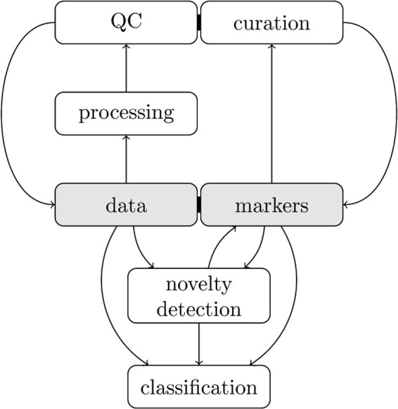
The steps leading to a sound analysis of spatial proteomics data.

Quantitative Data

The data that are generated via the typical spatial proteomics experimental designs can be represented in tabular format with features and fractions along rows and columns, respectively (as illustrated in Fig. 2, left). The features generally correspond to proteins or protein groups, although peptides can also be used. A second critical set of information is required for further data analysis, namely, organelle markers. These are proteins that are defined as reliable organelle residents and can be used as reference points to identify new members of that organelle. These marker proteins are generally selected by domain experts and play a central role in data analysis at many different levels, as highlighted in the next sections.

Fig. 2.

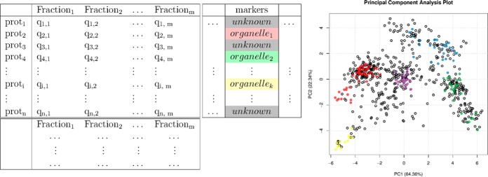
Left, representation of a fully described spatial proteomics dataset containing quantitative data for n proteins along m fractions. Each protein is described by additional metadata, in particular the definition of the known subcellular localization for well-known residents. Fractions are also decorated with specific metadata. Right, summarization of the quantitative data and annotation of the “markers” protein metadata using a principal component analysis figure.

The nature of the experimental design will characterize the size and the nature of the quantitative data in multiple ways. For example, there are technical advantages to multiplexing strategies such as isobaric labeling quantitation using iTRAQ (16) or TMT (17) labeling systems, but they directly reduce the resolution that can be measured along the separation dimension, as one is limited by the number of tags that can be employed to quantify fractions. This inherently limits the data cardinality and consequently reduces the discriminative power of subcellular niches with similar profiles, as illustrated in Fig. 3. These protein profiles represent well-characterized mitochondrial and endoplasmic reticulum residents from two different experiments, namely, a TMT 6-plex (red) and a label-free experimental (black) design, that have been fully quantified using 6 and 16 gradient fractions, respectively. The quantitation of more fractions using additional independent mass spectrometry acquisitions must be mitigated by the prevalence of incompletely characterized profiles (described in the section “Data Processing” and Fig. 4) due to missing values, which are rife in label-free datasets because of the semi-stochastic nature of data-dependent acquisition mass spectrometry approaches.

Fig. 3.

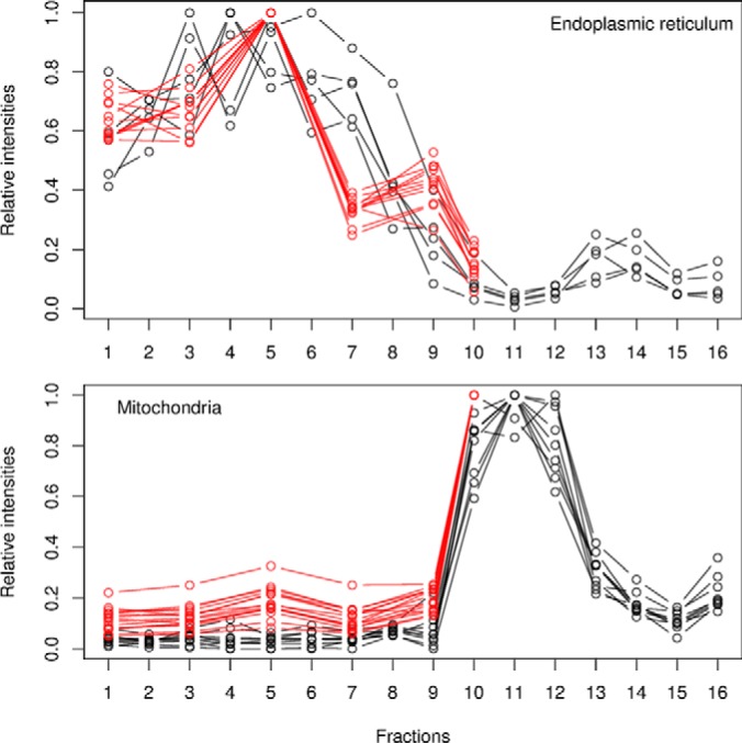
Effect of the number of fractions on the resolution along the separation gradient for the endoplasmic reticulum (ER) and mitochondria from a TMT experiment using 6 fractions (red) and the equivalent label-free experiment quantified along 16 fractions (black). The profiles are those of carefully selected Drosophila markers that were quantified in all the fractions. 15 and 11 fully characterized mitochondrial and ER markers were identified in the TMT dataset, whereas the label-free approach identified only 9 and 5 complete profiles because of missing values.

Fig. 4.

Assessment of data imputation on cluster resolution and protein organelle assignment. Left, the positive relation between number of imputed values and displacement of the points before (original values) and after imputation. In the PCA plot (right), the numbers of missing values that were imputed are reported in the protein points, and the effect on the change in position of the proteins in the PCA plot is highlighted by arrows that show a clear trend toward the origin of the plot.

In the following sections, we use published datasets from Dunkley et al. (7) and Tan et al. (18), using augmented marker sets described by Breckels et al. (19), in order to illustrate our findings. These datasets are also distributed as well-documented and computer-friendly data structures (13) in the pRolocdata (11) package and can be used as input to the software packages used to run the computational experiments described below. Both datasets mentioned above were derived through use of the LOPIT technique to localize integral and associated membrane proteins.

Dunkley et al. (7) prepared two independent Arabidopsis thaliana callus membranes and fractionated them by using self-generating iodixanol density gradients. For each preparation, two iTRAQ 4-plex tags (16) were used to quantify seven different fractions, with one fraction that was the same in both acquisitions. Firstly, fraction 1 (least dense) was labeled with reagent 114, fraction 4 with 115, and fraction 7 with 116, and fractions 11 and 12 were pooled and labeled with 117. Then, fraction 2 was labeled with iTRAQ reagent 114, fraction 5 with 115, fraction 8 with 116, and fractions 11 and 12 with 117. The total experiment yielded replicated measurements for eight quantitation values along the gradient. Labeled peptides were separated using strong cation exchange chromatography and analyzed via LC-MS/MS on a QSTAR XL quadrupole-time-of-flight mass spectrometer (Applied Biosystems, Foster City, CA). Tan et al. (18) collected Drosophila melanogaster embryos at 0 to 16 h. The material was homogenized and centrifuged to collect the supernatant, thereby removing cell debris and nuclei. Membrane fractionation was performed on an iodixanol gradient, and fractions were quantified using iTRAQ 4-plex isobaric tags (16) as follows: fractions 4/5, 114; fractions 12/13, 115; fraction 19, 116; and fraction 21, 117. Labeled peptides were then separated using strong cation exchange chromatography and analyzed via LC-MS/MS on a QSTAR XL quadrupole-time-of-flight mass spectrometer (Applied Biosystems).

Data Visualization

One can directly visualize the experimental data by plotting the protein intensities, or generally their relative intensities, along the separation dimension. Although very useful, this representation is limited by the number of proteins or clusters of proteins that can be represented in one figure. It is often essential to be able to visualize the full dataset in one figure, possibly in summarized form, in order to assess the underlying structure of the data and develop an intuition of what can reasonably be achieved in light of the data's properties. A popular technique for describing multivariate data is dimensionality reduction. This allows one to represent the data in a reduced set of dimensions, generally two or three, instead of the original higher number corresponding to the individual fractions (the columns of our data matrix represented in Fig. 2), while maintaining as much of the initial information as possible. Principal component analysis (PCA) or nonlinear versions thereof are procedures that transform the original data into a set of orthogonal components that are ordered according to the amount of variability that they describe (Fig. 2, right). For a well-structured dataset, representation as a projection along the two first components is often an effective means to obtain a simple yet representative visualization of the data. The first principal component, representing the most variability in the data, generally equates to the main separation dimension applied to the cell content. In addition, if one considers the amount of variability that is described along each of these first principal components, one can assess how faithfully this two-dimensional representation of the data describes the high-dimensional data. Note that relatively minor variances within the data can also be biologically relevant, and lower components may also be informative. Although this representation remains a simplification, it is often possible to gain notable understanding of a complex experiment from this single figure.

Data Processing

In this section, we discuss two essential aspects of data processing, namely, imputation of missing values and data normalization. Although it is rarely exposed, it is important to acknowledge the detrimental effect of missing values that are so prevalent when combining independent acquisitions. None of the machine learning algorithms that have been applied to organelle proteomics nor any of the contemporary machine learning methods can directly deal with incomplete data; missing values are always explicitly or implicitly imputed before submission to an algorithm. Missing data and the impact of imputation have not been thoroughly addressed in proteomics, let alone in spatial proteomics. Published LOPIT studies (7, 18, 20) have excluded proteins that presented missing values across replicated experiments. PCP studies (8, 21) have limited the computation of their χ² metric to pairs of fractions (defined as the squared deviation of the normalized profile for all peptides divided by the number of data points), thus increasing the bias by reducing the number of data points. Other studies have either explicitly (22) or implicitly (10) applied data imputation without necessarily assessing the biases of the procedure. To illustrate the issues of imputation of missing data, we assessed the impact of imputation using the specific goals of spatial proteomics (i.e. the identification of subcellular protein clusters and the assignment of proteins). In Fig. 4, we present data from Ref. 7, which provides complete profiles for 16 fractions (some being replicates) for nearly 700 proteins. After random assignment of missing values and data imputation using nearest neighbor imputation (23), we estimated the effect of the imputation method by tracking the shift of the imputed value with respect to the original data points. As expected, we noted an increasing effect of imputation on the data with an increasing number of missing values (Fig. 4, left). In addition, data imputation resulted in a translation of data toward the center of the figure, corresponding to less pronounced protein profiles across the gradient (Fig. 4, right). This trend is representative of a loss of signal resulting from imputation, which results in a reduction in the classification power and a bias toward misclassification to organelles that are characterized by such average profiles, such as plasma membrane in the example shown.

Data normalization is a topic that has been frequently explored in many areas of transcriptomics and proteomics, albeit never in the light of organelle proteomics data. In all subsequent analyses and visualizations we used relative intensities across the fractionation scheme. When absolute intensities are used for visualization, the absolute component of the signal will overwhelmingly influence the data transformations and eventually hide the relative signal that is of primary interest. All published research tends to divide each intensity by the maximum, or by the sum of intensities in each row of the data matrix. More work on the benefit of the application of more sophisticated techniques would be welcomed, in particular when multiple experimental conditions acquired during different runs ought to be compared (see “Translocalization”). Finally, as illustrated in Fig. 5, the accuracy and precision of the underlying quantitation methodology is an essential parameter for optimal cluster resolution (24), and advances in mass spectrometry technologies and quantitation protocols play a crucial role in the production of reliable data.

Fig. 5.

Effect of noise on subcellular cluster resolution. Comparison of original data from Dunkley et al. (7) (left) and data to which additional quantitation noise has been added (right). The quantitation noise was simulated by adding a normal error term (using the mean of the data and 1/2 standard deviation as parameters) to the quantitation data. Although the clusters are still visible and well separated in the noisy data, the original data feature much tighter and better resolved data with better separation boundaries between groups of interest.

Importance of Organelle Markers

An organelle marker is a protein known to be a resident of a specific subcellular niche in the species and condition of interest. From a computational point of view, markers allow the mapping of regions in the multidimensional data space to subcellular localizations (Fig. 2). The validity of markers, and thus the reliable mapping of biological information to the multivariate data, is generally ensured by expert curation of the proteins in the dataset. Gene Ontology (GO) (25), and in particular the cellular compartment (CC) namespace, is an essential starting point for protein annotation and marker definition. Nevertheless, automatic extraction of GO CC is only a first step, and additional curation is required to counter unreliable annotation based on data that are inaccurate or out of context for the biological question under investigation. Although proteins with genuine multiple localizations are of particular interest (see below), one must be careful when assessing multiple GO CC terms and distinguish proteins present in more than one subcellular niche (multilocalization) from changes in localization under different conditions and incorrect annotation. Annotations often represent a default/consensus state, whereas the information required to define a reliable marker is specific to the system under study and the conditions of interest. In particular, examples that do not match an annotated localization for biologically relevant reasons will be of remarkable interest. As a result, there is an inevitable trade-off that must be considered when using a very stringent high-confidence list or increasing the number of markers to better characterize the multivariate data. Both aspects are important, as a minimum number of markers is required for further data analysis and misassignment can have a detrimental effect on data analysis (see sections “Novelty Detection” and “Classification”), and a good balance can be obtained through careful quality assessment of the markers (next section).

Although marker definition is an important step, it is only the initial step of the analysis workflow and is often time consuming. To facilitate the identification of markers, we curated proteins and mined publicly available datasets (7, 8, 18–20, 22, 26, 27) to provide marker sets for Arabidopsis thaliana (543 markers, 13 organelles), Drosophila melanogaster (220 markers, 11 organelles), Saccharomyces cerevisiae (128 markers, 12 organelles), Gallus gallus (102 markers, 5 organelles), mouse (648 markers, 21 organelles), and human (507 markers, 16 organelles) as part of our software infrastructure (11) (see details in the supplemental material). These markers are now available in the pRoloc software and can be directly added to quantitative datasets. They are provided as a starting point for the generation of reliable sets of organelle markers but still need to be verified against any new data in light of the quantitative data and the study conditions.

Quality Control

The quality of the data is often evaluated using a set of dedicated quality metrics and/or through visualization. The use of unsupervised machine learning methods (clustering) that represent the quantitative data without additional external qualitative information is an efficient approach. Our first quality assessment aims at verifying whether the first principle behind gradient-based organelle proteomics is met. Based on De Duve's principle (28), we expect that proteins that share the same subcellular localization should co-localize across a fraction scheme, resulting in well-defined structure in the data. We routinely apply the PCA representation described above, without any additional information (symbols colored depending on external information such as organelle residency), to inspect the data and assess whether structure can be observed. In a first instance, overlaying markers can be misleading by conferring a false sense of data structure and should be avoided so that the data can be inspected in a completely unsupervised way; the first quality assessment ought to inform on the existence of clusters and structure of data prior to the mapping on biologically relevant niches. If no structure is present, even if coherent marker groups can be identified, one should not expect well-defined classification boundaries that separate the subcellular clusters, and thus interpretation of data points located in the continuous cloud of points separating two clusters will be challenging. A second assessment laid out by the experimental design can be explored by overlaying meta-data on the PCA plot, in particular organelle markers. These should match, to some extent, the underlying data structure and explain some, but not necessarily all, of the observed protein clusters. An important question arises when marker proteins show substantial deviation from the rest of the group, or more generally when a supposedly well-defined cluster shows a widespread, undefined distribution. Consistent lack of structure/clusters in the data is often indicative of poor separation and undermines all subsequent analysis and interpretation. When individual outliers are detected, it is advised to verify the reliability of the data (identification and quantitation accuracy) and annotation trustworthiness. When any of these can be questioned, the annotation or possibly the protein altogether might be removed from the data. If neither misidentification nor unreliable quantitation can explain the unexpected position of the marker, it will be the experimenters' responsibility to decide whether to unlabel the protein (i.e. not consider it as a reliable marker despite anticipated localization and reliable identification/quantitation) or keep it as is and instruct subsequent algorithms of a possible extended mapping of the organelle to the data. It is, however, important to note that a marker's localization cannot be (automatically) undone during the data analysis (it represents a rigidly imposed constraint that anchors the data space), whereas an unlabeled protein can be assigned any of the identified localizations. A possible approach could be to unlabel the unreliable marker and verify whether it eventually gets assigned to the expected localization. The drawback of a systematic application of this approach is an underrepresentation of the multidimensional data space: unlabeling markers corresponds to a loss of information, and it is, in the end, up to the expert to decide whether the information is reliable and on what grounds it should or should not be trusted in light of the data and their quality.

It is important to highlight that it is generally not possible, or desirable, to identify the complete subcellular diversity using markers at this stage. In general, reliable markers can easily be identified for large and well-studied niches. The nature of supervised machine learning methods that have been used to date in organelle proteomics studies (see “Classification”) constrains assignments of proteins to a set of marker classes. As a result, there is a need for discovery of new data-specific and relevant localization clusters using a reduced set of highly reliable markers and the underlying structure of our quantitative data.

Novelty Detection

The assignment of proteins to organelles in spatial proteomics traditionally relies on supervised multivariate statistical and machine learning analysis wherein a set of highly curated organelle markers (labeled training data) that belong to a finite set of organelles is used to map gradient profiles of unknown localization to subcellular localizations with high accuracy. The application of such methods, however, is often hindered by failure to extract organelle markers that cover the whole subcellular diversity in the data; this leads to prediction errors, as protein profiles of unknown localization can only be associated with organelles that appear in the labeled training data. The extraction of all organelle and organelle-related clusters is a difficult task owing to the limited number of marker proteins that exist in databases and elsewhere and the time-consuming nature of obtaining reliable markers. To address these issues, Breckels et al. (19) developed a novelty detection algorithm that is able to identify subcellular groupings such as organelles and protein complexes in spatial proteomics experiments. The algorithm, phenoDisco, uses a semi-supervised machine learning schema that employs iterative cluster merging combined with Gaussian mixture modeling and outlier detection to identify putative subcellular compartments. In a semi-supervised scenario, a classifier is learned in the presence of both labeled (i.e. organelle markers) and unlabeled (i.e. proteins of unknown localization) data. In order to apply Breckels's algorithm, one requires an initial set of high-quality input organelle markers that cover a minimum of two classes, each containing six or more marker protein profiles, and of course some unlabeled data that can be mined for new phenotype organelle clusters.

The choice of labeled data (i.e. organelle markers) from which the applied machine learning system will learn is extremely important, as it can have a significant effect on the success or failure of the learner. To illustrate this paradigm, we investigated the effect that marker choice has upon the application of the phenoDisco novelty detection algorithm in mining a Drosophila melanogaster dataset that had been produced using the LOPIT technology (18). We considered three sources of markers for use as input for the phenoDisco algorithm: (i) a highly and manually curated set from experts in the field (20 endoplasmic reticulum (ER), 6 Golgi, 14 mitochondrial, and 15 plasma membrane markers from our curated marker sets, originally obtained from Ref. 18); (ii) unique GO CC annotations assigned a localization based on experimental evidence plus those assigned a unique localization as inferred from structural sequence or similarity in the GO database; and (iii) only unique GO CC annotations assigned a localization based on experimental evidence in the GO database. Reassuringly, it was found that in case i, where a small set of manually curated markers were used as input, six out of the seven previously unlabeled phenotype clusters that were found in the phenoDisco experiments published in Ref. 19 were identified: a cluster of proteins that represented two ribosomal subunits (40S and 60S), nucleus, proteasome, lysosome, and the cytoskeleton. An additional cluster of cytoplasmic proteins was also identified (phenotype 7, Fig. 6A, right). Remarkably, we found that the use of organelle marker set ii had a detrimental effect on the ability of the algorithm to identify any new organelle clusters, and we were able to identify only one new phenotype (Fig. 6B, right). Examination of the organelle markers in set ii showed a lack of cluster resolution and overlap of the Golgi apparatus, plasma membrane, and ER (Fig. 6B, left). We also found a mitochondrial outlier in the dataset that was completely separated from the other mitochondrion markers and located toward the ER cluster. It was found that the inclusion of this one clear outlier forced a negative constraint on the phenotype modeling, which resulted in a lack of new phenotypes detected. In an attempt to improve marker list ii, we considered marker set iii, which included unique GO CC annotations assigned based on experimental evidence only. We identified 6, 0, 11, and 15 markers for the ER, Golgi apparatus, mitochondrion, and plasma membrane, respectively. These presented minimal overlap with the curated markers (only three for the mitochondrion and plasma membrane). We observed a significant improvement in organelle cluster detection (Fig. 6C, right). We did, however, see more noise in the form of a number of smaller phenotypes that lay on the edge of the ER cluster. Interestingly, we also noted that the phenoDisco algorithm detected the Golgi as an independent phenotype (phenotype 10, Fig. 6C, right). No unique Golgi CC markers were retrieved from the GO that were assigned from experimental evidence that could be used as input markers in set ii; thus it is reassuring that we were still able to retrieve this organelle using novelty detection methods. An important step in the application of any novelty detection algorithm is the careful examination of the protein content of any new clusters identified. Curation and examination by experts in the field is an essential step in the discovery analysis pipeline. Using such approaches, a researcher is able to mine MS datasets at a deeper level and bring to light interesting subcellular compartments for more comprehensive validation for use in a supervised machine learning analysis for robust protein localization assignment.

Fig. 6.

The effect of different organelle marker sets (left) on the application of the novelty discovery algorithm phenoDisco (right) in mining a Drosophila melanogaster dataset produced using the LOPIT technology (18). A, a set manually curated by experts in the field. B, unique GO CC annotations from experimental evidence or computational predictions. C, unique GO CC annotations from experimental evidence.

Classification

In machine learning, the task of classification falls under the broad area of supervised learning. In supervised learning, the aim is to train a classifier to learn a mapping between a set of observed instances and a set of associated external attributes that are being predicted (usually known as the class label or predictor). This set of instances, along with their known class labels, is typically called the training data. Once a classifier has been learned from the training data, the aim is to use this classifier to predict the class labels on data with unknown attributes. All methods to date that have been applied to predict protein localization have used supervised machine learning.

In terms of protein localization prediction using data from MS-based organelle proteomics experiments, each training data example consists of a pair of inputs: the actual data, generally represented as a vector of numbers (such as the associated normalized ion intensities along a set of fractions for a given protein), and a class label, representing the membership to exactly one of multiple possible organelle classes (this is usually referred to as a multiclass problem). When there are only two possible classes, this is referred to as binary classification. Before one can generate a model on the training data and classify unknown residents, one has to properly set the model parameters. Wrongly set parameters can have adverse effects on the classification performance and success of the learner to the same degree as inappropriate training examples. An important factor to consider in one's choice of training examples (i.e. organelle markers) is how well they represent the multivariate data space (i.e. the distribution of proteins over which the system's performance will be measured). In general, it has been found that learning is most reliable when the training data follow a distribution similar to that of the examples to be classified.

Parameter optimization can be conducted in a number of ways. One of the most common ways to optimize one's parameters is to use the convention of a training set (to model) and a testing set (to predict) that are subsets extracted from the labeled training data. Observed and expected classification results can be compared and then used to assess how well a given model works by providing an estimate of the classifier's ability to achieve a good generalization (that is, given an unknown example, predict its class label with high accuracy). A commonly used measure of classifier performance is the macro F1 score, $F1=2\frac{precision\times recall}{precision+recall}$, which is the harmonic mean of $precision=\frac{tp}{tp+fp}$ and $recall=\frac{tp}{tp+fn}$, where tp = true positives, tn = true negatives, fp = false positives, and fn = false negatives. This procedure is usually used for a range of possible model parameter values (this is called a grid search), and the best performing set of parameters is then used to construct a model on all markers and predict unlabeled proteins. Estimation of the algorithmic performance can be assessed in many ways, such as via cross-validation. In the pRoloc package, algorithmic performance is estimated using stratified 20/80 partitioning in conjunction with 5-fold cross-validation in order to optimize the free parameters via a grid search. This procedure is usually repeated 100 times, and then the best parameters are selected upon investigation of associated macro F1 scores. A high macro F1 score indicates that the marker proteins in the test dataset are consistently correctly assigned by the algorithm. Often more than one parameter or set of parameters gives rise to the best generalization accuracy. Thus it is always important to investigate the model parameters and critically assess the best choice. The best choice might not be as simple as the parameter set that gives rise to the highest macro F1 score, and one must be careful to avoid overfitting and to choose parameters wisely.

Once the best parameters have been selected, they can be used to build a classifier from the training data of organelle markers. The classifier will return a classification result for all unlabeled instances in the dataset corresponding to their most likely subcellular compartment. In addition, it is possible to extract classification accuracy scores that can inform on the reliability of the assignment. Many supervised machine learning algorithms have been developed, some of the most popular being the support vector machine (SVM), k-nearest neighbor, random forest, neural networks, and naive Bayes, among others. These methods, along with newer state-of-the-art algorithms such as the Perturbo (29) classification algorithm, are available in the pRoloc package. With the vast number of classification methods available, it is often a daunting task to choose the method that is best suited to the classification task; however, it is not often the choice of algorithm that underpins robust results. In fact, it is widely accepted that it is not algorithm choice that matters but the way in which the algorithm is applied and the availability of good training data.

As an example of an application of protein localization prediction using supervised machine learning, we took the first replicate from Tan et al. (18) and applied a weighted SVM classifier for protein classification. The labeled training data (Fig. 7, left) were constructed from manually curated markers from Ref. 18, which were further refined using Breckels et al.'s (19) phenotype discovery algorithm. Here, using the pRoloc package, we employed a weighted SVM with a Gaussian kernel to learn a nonlinear decision function on the training data to map proteins of unknown localization to one of the known organelle classes. Class specific weights were used when creating the SVM model and were set to be inversely proportional to the class frequencies to account for class imbalance. On the training data, the two free SVM parameters, cost and sigma, were optimized over 100 rounds of stratified 5-fold cross-validation via a grid search, and the best pair of parameters for the classifier were chosen from evaluation of the macro F1 scores (Fig. 7, middle). The optimized SVM classifier was then used to predict protein localization on the unlabeled data (Fig. 7, right). The sizes of the points in Fig. 7 (right) reflect the classification probabilities.

Fig. 7.

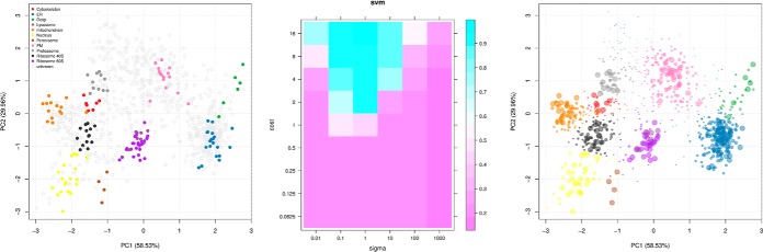
Application of the support vector machine classifier (SVM) to the data from Tan et al. (18). Left, augmented dataset after novelty detection. Middle, grid search for the SVM parameter cost and sigma, highlighting optimal pairs of parameters. Right, application of the SVM classifier. The size of the point reflects the classification probability.

Multiple Conditions and Multi-localization

The previous sections demonstrate a robust protocol allowing one to mine and understand data, verify its annotation, and explore it to identify new clusters and classify proteins to subcellular niches, relying on state-of-the-art algorithms and proven methodologies. Additional complexity arises when multiple conditions need to be considered in order to elucidate the dynamic nature of protein localization or multi-localization of proteins to multiple subcellular compartments. To illustrate key concepts and pitfalls of such analyses, we generated a set of controlled localization changes using the experiments of Dunkley et al. (7) and relevant curated marker proteins. We modeled changes in localizations and moved proteins from one organelle to another by updating their observed quantitative data along the gradient with new meaningful values inferred from the same dataset.

Multi-localization

The protein databases provide multiple localization annotations per protein in about 60% of human UniProt entries (see the supplemental material). Although a certain number of these annotations are likely to be erroneous or represent specialization of identical compartments and do not necessarily imply that proteins multi-localize under identical conditions, dual-localization is an important aspect that needs to be addressed. We used the complete data from Ref. 7 to create a variable mixture of protein relative abundances along the gradient to simulate dual-localization. Fig. 8 (left) shows such an example in which all fractions of ER (blue) and plastid (orange) marker protein profiles have been combined to generate a set of ER/plastid mixtures ranging from only ER to only plastid through 90% ER/10% plastid, 80% ER/20% plastid, …, 10% ER/90% plastid intermediates. The resulting mixture profiles are represented as points on the global PCA plot (Fig. 8, right) and are colored according to their classification using an SVM classifier and the procedure described in the section “Classification.” As can be seen, some of the mixtures travel over the plasma membrane cluster, localized between the end points on the PCA plot, and are classified accordingly. The sizes of the points along the mixture gradient are proportional to the classification probabilities. ER–plastid mixtures that closely match plasma membrane profiles are classified as plasma membrane residents. A plasma membrane marker protein is represented in yellow in the mixture profiles (Fig. 8, left) to illustrate the relevance of the classification result. Various mixtures for other dual-localization scenarios have been modeled and lead to identical scenarios in which intermediate mixtures match intermediate organelle profiles (see the supplemental material).

Fig. 8.

Application of the SVM classification algorithm to identify dual-localization patterns. Left, ER (blue)–plastid (orange) relative quantitation mixture. A plasma membrane marker protein is shown in yellow. Right, position of the respective ER–plastid mixtures on the PCA plot and their respective color-coded classifications.

Despite the fact that the PCA plot is a two-dimensional projection of the data, the results of the nonlinear classifier are accurately described for these well-resolved data. These simulations indicate that proportional mixtures of two well-defined organelle members that mimic dual-localization of proteins at various proportions are easily confounded with other subcellular compartments. From this result, we deduce that reliable inference of dual- and more generally multi-localization requires additional biological information and cannot rely only on unique proteins. In particular, we suggest that known dual-localized examples that form coherent clusters are desired to reliably identify new examples; single evidence proteins can hardly be distinguished from quantitation noise or from membership in intermediate compartments.

Trans-localization

To simulate multiple conditions, we took advantage of the availability of biological replicates in Ref. 7. The two membrane preparations exhibit technical variability that represents a considerable challenge when investigating genuine changes in localization, thus making this example a faithful representation of real use cases, while allowing us to set and control protein trans-localizations. We chose seven marker proteins (see the supplemental material for details) and imposed changes to different destination organelles. The original relative quantitation values were replaced by the mean fraction values of all destination marker proteins. The trans-localizations are highlighted by arrows in Fig. 9. Below, we demonstrate important aspects influencing the analysis of dynamic spatial proteomics data, namely, data normalization, the identification of trans-localization, and concerted trans-localizations.

Fig. 9.

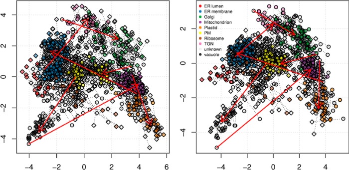
Application of the variance stabilization normalization of two replicates (circles and diamonds) of our test data. The solid red arrows indicate the trans-localized proteins. Left, original data showing substantial differences between replicates 1 (circles) and 2 (diamonds). The colors represent all markers for the nine subcellular localizations. After application of the normalization procedure (right), we obtained considerably better overlap between the replicates.

Data Normalization

The two replicates displayed both biological and substantial technical variability, as illustrated in Fig. 9 (left). The first and second replicates are represented by circles and diamonds, respectively, and the corresponding pairs of proteins are linked by dotted segments. The colors represent all marker proteins for the nine subcellular niches identified for this dataset. Although the mass spectrometry processing is becoming more reliable and reproducible, the density separation gradient is a sensitive operation that is executed manually. Trotter et al. (9) have demonstrated that combining different gradients that separate different sets of organelles from replicated measures from a single condition achieves a better separation than each gradient taken separately, but it is still essential to reduce intracondition variability to highlight differences between conditions. We transformed the data using variance stabilization normalization (30), a technique that has already been successfully applied to proteomics data (31). The result is represented in the right-hand panel of Fig. 9 and shows a substantial improved overlap of replicates 1 (circles) and 2 (diamonds).

Identifying Trans-localizations

We combined two complementary procedures to search for the seven trans-localized proteins. We employed the machine learning tools described earlier and performed a classification analysis on two replicates with the trans-localized proteins. As shown in Table I, the two replicates mostly agreed (values along the diagonal). There were, however, 107 other discrepancies, including the seven anticipated trans-localized proteins, that were assigned the expected localizations in each replicate (see the supplemental material).

Table I. Comparison of the classification results of two replicated experiments including simulated trans-localizations from Dunkley et al. (7). Values along the diagonal correspond to identical outcomes, and values in the upper and lower parts of the contingency table represent differences, seven of which were expected based on the imposed subcellular changes.

	ER lum	ER mb	GO	MT	PT	PM	Ribo	TGN	VA
ER lum	16	6	0	0	0	0	1	0	1
ER mb	0	175	3	0	0	9	5	1	0
GO	0	1	81	1	0	6	0	10	0
MT	0	0	0	81	9	2	0	0	0
PT	0	1	1	4	47	0	0	0	0
PM	0	4	5	4	0	98	5	1	2
Ribo	0	4	0	0	0	11	38	0	1
TGN	0	0	7	0	0	0	0	14	0
VA	1	0	0	1	0	0	0	0	29

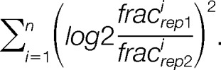
We next devised a second selection criterion, based on the rationale that trans-localizing proteins should be characterized by different quantitation profiles along the gradient. For each pair of proteins in the replicates, we summed the squared differences of the respective fraction log₂ ratios:

The distribution of these distances is shown in Fig. 10 (left). The distances corresponding to the seven trans-localized proteins are shown in blue. Three of these proteins are clear outliers (above the red dashed line, corresponding to the largest non-trans-localized protein). If we consider the smallest trans-localized distance (black dashed line), nine non-trans-localized proteins display larger distances. These nine pairs of proteins are highlighted in red on the PCA plot in Fig. 10; five pairs show differently colored starting circles (replicate 1) and ending diamonds (replicate with trans-localizations), representing false positives (see details in the supplemental material).

Fig. 10.

Identification of changes in localization. Left, distribution of the summed squared log₂ ratios between fractions of the two conditions of interest. Blue points represent genuine trans-localizations. The red and black dashed lines represent the largest non-trans-localized value and the smallest genuine trans-localized protein. Right, PCA plot illustrating effects of technical variability and trans-localizations. Non-trans-localized pairs with a sum of squared log₂ ratios greater than genuine changes are highlighted in red, and genuine trans-localizations are represented by thick arrows.

Although all seven trans-localizations were classified as expected and displayed considerably greater sums of squared log₂ ratios than most other proteins, a notable proportion of false positives were present among the top hits. Only proteins exhibiting extreme trans-localization distances between subcellular locations that span the full width of the separation capabilities of the design are likely to be reliably identified. Such mixed results are likely to be generalizable because of the high variability during cell content separation.

Concerted Trans-localizations

Although it is difficult to identify genuine single trans-localizing proteins, a biologically relevant scenario could imply a set of proteins exhibiting the same event of trans-localization, termed concerted trans-localization. We modeled such a case by trans-locating 15 mitochondrial proteins (purple) to the plastid cluster (orange) (Fig. 11, left). The new positions were generated by adding small amounts of normal noise to 15 plastidial residents. Although the changes in localization are correctly classified (see the supplemental material), the trans-localization distances are not large enough to be differentiated from the technical and biological variability between replicates, as anticipated from our previous results. However, we predicted that it should be possible to identify the synchronized displacement of the candidates. To do so, we counted the number of trans-localizations between all possible pairs or organelles (Fig. 11, top heatmap). We then normalized these counts by subtracting reciprocal pairs to balance gain and loss of residents (Fig. 11, bottom heatmap). For example, six changes are documented from ER membrane to the ribosome and five from the ribosome to the ER membrane, resulting in a net change of 1 in favor of the ER membrane. Indeed, gains and losses should compensate each other in the case of random fluctuations, whereas consistent movements produce a systematic decrease and increase of recorded events at the origin and destination of the concerted trans-localizations. The normalized number of trans-localizations reported our expected count of mitochondrion to plastid movements. We also observed that up to eight random net displacements could be observed and that the appearance of concerted trans-localization was only apparent when enough proteins displayed synchronized behavior.

Fig. 11.

A scenario of concerted trans-localization involving 15 proteins moving from the mitochondrial organelle (purple) to the plastid cluster (orange). Random trans-localizations are connected by red dotted segments. The heatmaps show the absolute (top) and normalized (bottom) number of observed trans-localization effects. Concerted trans-localization effects are characterized by high net gains and reciprocal losses of displacements.

DISCUSSION

We have described a typical pipeline of organelle proteomics data and clarified some central machine learning concepts applied to such data. It is essential to understand the principles, requirements, weaknesses, and strengths underpinning such analyses before confidently interpreting the results, but the availability of the right tools is also essential. A recent review by Drissi et al. (32) presents an overview of proteomics methods for subcellular proteome analysis. In a section about bioinformatics tools for the analysis of organelle proteomics data, they do not mention the existence of any software that will allow the analysis of such data and only refer to the importance of existing protein subcellular annotations and the role of GO. It is interesting to look back on past studies and note which methods have been used and also whether, with hindsight, improvements could have been made in the application of approaches and the reporting of data. This is a useful exercise to undertake, especially in such an emerging field as spatial proteomics data analysis. The first applications of large-scale organelle proteomics data analysis were protein correlation profiling efforts (8, 21) that calculated the χ² metric using in-house tools and LOPIT (7, 18, 20) that applied partial least squares discriminant analysis using the commercial SIMCA software (Umetrics, Umea, Sweden). Trotter et al. (9) implemented custom R code (12) and used the SVM algorithm from the kernlab package (33), but no code for others to repeat this state-of-the-art procedure is provided. Others have applied other contemporary machine learning algorithms, including random forests (10), naive Bayes (22), and neutral networks (34), but did not provide means to apply their analyses to new data. Although proteomics data are commonly being disseminated through appropriate repositories, it is not commonplace to provide reproducibility in terms of software and data analysis, despite their recognized importance (35).

Here we have attempted to redress access to code and the ability to reproduce data analysis by performing the analysis and creating illustrations using the R language and a set of well-documented Bioconductor (14) software add-ons specifically developed for quantitative proteomics data. The MSnbase package (13) allows the consistent management and processing of quantitative data and associated metadata, and the pRoloc package (11) provides a visualization and statistical machine learning (including all the algorithms mentioned above, as well as novel ones (29)) framework to analyze and interpret spatial proteomics data. The software allows the implementation of a robust and reproducible analysis pipeline and is flexible enough to accommodate various designs and foster the development of innovative analysis strategies. The software provides extensive documentation and tutorials for a fully reproducible organelle proteomics framework. Finally, pRoloc benefits from the Bioconductor infrastructure and its full integration with various online resources, including, among many others, the Gene Ontology (the GO.db package (36)), the UniProt database (the biomaRt package (37)), and the Human Protein Atlas (38, 39) (the hpar package (40)).

In this study we also sought to develop analysis pipelines that will be useful to dual-/multi- and trans-localization study designs. Such approaches build on robust single condition classification accuracy that relies on good resolution of the subcellular space to reduce inter-organelle variability (well-defined clusters) and enable reliable organelle assignments. Trans-localization studies over additional conditions suffer from additional levels of variability that can partially be addressed in multiple ways. First, the use of biological knowledge, including dual-localized or concerted dynamic protein markers, can be used to direct the supervised components of the analyses while providing a reliable starting point for uncovering genuine signal from noise. Second, the reduction of technical variability through adequate normalization (see the section “Trans-localization”) or multiplexed designs will be of paramount importance. The balance between the number of fractions and the advantage of multiplexing strategies to reduce inter-run variability and missing data discussed in the section “Quantitative Data” becomes even more critical in multi-condition designs, when relying on three (TMT 6-plex) or four (iTRAQ 8-plex) fractions per condition makes it challenging to obtain any well-resolved clusters in the data. The advent of higher multiplexing solutions, such as TMT 10-plex, promises to optimize dynamic designs by combining sufficient resolution and reducing technical variability. Finally, replication can confer more accurate classification in single conditions (9) and will provide an assessment of uncertainty to support the identification of multi- and trans-localization events.

CONCLUSION

The path to reliable data analysis results is never written in stone, in particular for complex experimental designs and multivariate data. There are, however, certain requirements that are always applicable. Visualization of the complete dataset is essential in order to describe its major features; in the case of a spatial proteomics experiment, we have highlighted multiple applications of dimensionality reduction techniques such as PCA. This is, of course, a simplification of the complete data, but it can provide a first inkling of the extent of separation and success of classification. It is also important to set basic assumptions about the data, assess the organelle markers in light of the data structure, describe how it is processed, and assess the effects of the treatments it undergoes. Finally, the extent to which the result of the data classification algorithm is reliable must be questioned. Trust in the results will be gained through the proper usage of algorithms, quality control of the data, and verification that basic assumptions about the data (e.g. appropriate separation of the data, reliable usage of markers, consideration of biologically relevant diversity) and the algorithms in terms of adequate utilization and parameter selection are met. The methodology that we have demonstrated brings us a step closer to meeting the requirements of a trustworthy spatial proteomics data analysis.

REFERENCES

- 1. Dreger M. (2003) Subcellular proteomics. Mass Spectrom. Rev. 22, 27–56 [DOI] [PubMed] [Google Scholar]
- 2. Park S., Yang J. S., Shin Y. E., Park J., Jang S. K., Kim S. (2011) Protein localization as a principal feature of the etiology and comorbidity of genetic diseases. Mol. Syst. Biol. 7, 494. [DOI] [PMC free article] [PubMed] [Google Scholar]
- 3. Luheshi L. M., Crowther D. C., Dobson C. M. (2008) Protein misfolding and disease: from the test tube to the organism. Curr. Opin. Chem. Biol. 12, 25–31 [DOI] [PubMed] [Google Scholar]
- 4. Laurila K., Vihinen M. (2009) Prediction of disease-related mutations affecting protein localization. BMC Genomics 10, 122. [DOI] [PMC free article] [PubMed] [Google Scholar]
- 5. Kau T. R., Way J. C., Silver P. A. (2004) Nuclear transport and cancer: from mechanism to intervention. Nat. Rev. Cancer 4, 106–117 [DOI] [PubMed] [Google Scholar]
- 6. Gatto L., Vizcaíno J. A., Hermjakob H., Huber W., Lilley K. S. (2010) Organelle proteomics experimental designs and analysis. Proteomics 10, 3957–3969 [DOI] [PubMed] [Google Scholar]
- 7. Dunkley T. P. J., Hester S., Shadforth I. P., Runions J., Weimar T., Hanton S. L., Griffin J. L., Bessant C., Brandizzi F., Hawes C., Watson R. B., Dupree P., Lilley K. S. (2006) Mapping the Arabidopsis organelle proteome. Proc. Natl. Acad. Sci. U.S.A. 103, 6518–6523 [DOI] [PMC free article] [PubMed] [Google Scholar]
- 8. Foster L. J., Hoog C. L. d., Zhang Y., Zhang Y., Xie X., Mootha V. K., Mann M. (2006) A mammalian organelle map by protein correlation profiling. Cell 125, 187–199 [DOI] [PubMed] [Google Scholar]
- 9. Trotter M. W. B., Sadowski P. G., Dunkley T. P. J., Groen A. J., Lilley K. S. (2010) Improved sub-cellular resolution via simultaneous analysis of organelle proteomics data across varied experimental conditions. Proteomics 10, 4213–4219 [DOI] [PubMed] [Google Scholar]
- 10. Ohta S., Bukowski-Wills J. C., Sanchez-Pulido L., Alves F. L., Wood L., Chen Z. A., Platani M., Fischer L., Hudson D. F., Ponting C. P., Fukagawa T., Earnshaw W. C., Rappsilber J. (2010) The protein composition of mitotic chromosomes determined using multiclassifier combinatorial proteomics. Cell 142, 810–821 [DOI] [PMC free article] [PubMed] [Google Scholar]
- 11. Gatto L., Breckels L. M., Wieczorek S., Burger T., Lilley K. S. (2014) Mass-spectrometry-based spatial proteomics data analysis using pRoloc and pRolocdata. Bioinformatics 30, 1322–1324 [DOI] [PMC free article] [PubMed] [Google Scholar]
- 12. R Core Team (2013) R: A Language and Environment for Statistical Computing, R Foundation for Statistical Computing, Vienna, Austria [Google Scholar]
- 13. Gatto L., Lilley K. S. (2012) MSnbase—an R/Bioconductor package for isobaric tagged mass spectrometry data visualization, processing and quantitation. Bioinformatics 28, 288–289 [DOI] [PubMed] [Google Scholar]
- 14. Gentleman R. C., Carey V. J., Bates D. M., Bolstad B., Dettling M., Dudoit S., Ellis B., Gautier L., Ge Y., Gentry J., Hornik K., Hothorn T., Huber W., Iacus S., Irizarry R., Leisch F., Li C., Maechler M., Rossini A. J., Sawitzki G., Smith C., Smyth G., Tierney L., Yang J. Y. H., Zhang J. (2004) Bioconductor: open software development for computational biology and bioinformatics. Genome Biol. 5, 80. [DOI] [PMC free article] [PubMed] [Google Scholar]
- 15. Yan W., Hwang D., Aebersold R. (2008) Quantitative proteomic analysis to profile dynamic changes in the spatial distribution of cellular proteins. Methods Mol. Biol. 432, 389–401 [DOI] [PubMed] [Google Scholar]
- 16. Ross P. L., Huang Y. N., Marchese J. N., Williamson B., Parker K., Hattan S., Khainovski N., Pillai S., Dey S., Daniels S., Purkayastha S., Juhasz P., Martin S., Bartlet-Jones M., He F., Jacobson A., Pappin D. J. (2004) Multiplexed protein quantitation in Saccharomyces cerevisiae using amine-reactive isobaric tagging reagents. Mol. Cell. Proteomics 3, 1154–1169 [DOI] [PubMed] [Google Scholar]
- 17. Thompson A., Schäfer J., Kuhn K., Kienle S., Schwarz J., Schmidt G., Neumann T., Johnstone R., Mohammed A. K. A., Hamon C. (2003) Tandem mass tags: a novel quantification strategy for comparative analysis of complex protein mixtures by MS/MS. Anal. Chem. 75, 1895–1904 [DOI] [PubMed] [Google Scholar]
- 18. Tan D. J., Dvinge H., Christoforou A., Bertone P., Martinez A. A., Lilley K. S. (2009) Mapping organelle proteins and protein complexes in Drosophila melanogaster. J. Proteome Res. 8, 2667–2678 [DOI] [PubMed] [Google Scholar]
- 19. Breckels L. M., Gatto L., Christoforou A., Groen A. J., Lilley K. S., Trotter M. W. (2013) The effect of organelle discovery upon sub-cellular protein localisation. J. Proteomics 88, 129–140 [DOI] [PubMed] [Google Scholar]
- 20. Hall S. L., Hester S., Griffin J. L., Lilley K. S., Jackson A. P. (2009) The organelle proteome of the DT40 lymphocyte cell line. Mol. Cell. Proteomics 8, 1295–1305 [DOI] [PMC free article] [PubMed] [Google Scholar]
- 21. Andersen J. S., Wilkinson C. J., Mayor T., Mortensen P., Nigg E. A., Mann M. (2003) Proteomic characterization of the human centrosome by protein correlation profiling. Nature 426, 570–574 [DOI] [PubMed] [Google Scholar]
- 22. Nikolovski N., Rubtsov D., Segura M. P., Miles G. P., Stevens T. J., Dunkley T. P., Munro S., Lilley K. S., Dupree P. (2012) Putative glycosyltransferases and other plant Golgi apparatus proteins are revealed by LOPIT proteomics. Plant Physiol. 160, 1037–1051 [DOI] [PMC free article] [PubMed] [Google Scholar]
- 23. Troyanskaya O., Cantor M., Sherlock G., Brown P., Hastie T., Tibshirani R., Botstein D., Altman R. B. (2001) Missing value estimation methods for DNA microarrays. Bioinformatics 17, 520–525 [DOI] [PubMed] [Google Scholar]
- 24. Jakobsen L., Vanselow K., Skogs M., Toyoda Y., Lundberg E., Poser I., Falkenby L. G., Bennetzen M., Westendorf J., Nigg E. A., Uhlen M., Hyman A. A., Andersen J. S. (2011) Novel asymmetrically localizing components of human centrosomes identified by complementary proteomics methods. EMBO J. 30, 1520–1535 [DOI] [PMC free article] [PubMed] [Google Scholar]
- 25. Ashburner M., Ball C. A., Blake J. A., Botstein D., Butler H., Cherry J. M., Davis A. P., Dolinski K., Dwight S. S., Eppig J. T., Harris M. A., Hill D. P., Issel-Tarver L., Kasarskis A., Lewis S., Matese J. C., Richardson J. E., Ringwald M., Rubin G. M., Sherlock G. (2000) Gene Ontology: tool for the unification of biology. The Gene Ontology Consortium. Nat. Genet. 25, 25–29 [DOI] [PMC free article] [PubMed] [Google Scholar]
- 26. Harner M., Körner C., Walther D., Mokranjac D., Kaesmacher J., Welsch U., Griffith J., Mann M., Reggiori F., Neupert W. (2011) The mitochondrial contact site complex, a determinant of mitochondrial architecture. EMBO J. 30, 4356–4370 [DOI] [PMC free article] [PubMed] [Google Scholar]
- 27. Ferro M., Brugière S., Salvi D., Seigneurin-Berny D., Court M., Moyet L., Ramus C., Miras S., Mellal M., Le Gall S., Kieffer-Jaquinod S., Bruley C., Garin J., Joyard J., Masselon C., Rolland N. (2010) AT CHLORO, a comprehensive chloroplast proteome database with subplastidial localization and curated information on envelope proteins. Mol. Cell. Proteomics 9, 1063–1084 [DOI] [PMC free article] [PubMed] [Google Scholar]
- 28. De Duve C., Beaufay H. (1981) A short history of tissue fractionation. J. Cell Biol. 91(3 Pt 2), 293s–299s [DOI] [PMC free article] [PubMed] [Google Scholar]
- 29. Courty N., Burger T., Laurent J. (2011) PerTurbo: a new classification algorithm based on the spectrum perturbations of the Laplace-Beltrami operator. In Proceedings of ECML/PKDD (1) (Gunopulos D., Hofmann T., Malerba D., Vazirgiannis M., eds), Vol. 6911, pp. 359–374, Springer, Berlin Heidelberg [Google Scholar]
- 30. Huber W., von Heydebreck A., Sültmann H., Poustka A., Vingron M. (2002) Variance stabilization applied to microarray data calibration and to the quantification of differential expression. Bioinformatics 18 Suppl 1, S96–S104 [DOI] [PubMed] [Google Scholar]
- 31. Karp N. A., Huber W., Sadowski P. G., Charles P. D., Hester S., Lilley K. S. (2010) Addressing accuracy and precision issues in iTRAQ quantitation. Mol. Cell. Proteomics 9, 1885–1897 [DOI] [PMC free article] [PubMed] [Google Scholar]
- 32. Drissi R., Dubois M. L., Boisvert F. M. (2013) Proteomics methods for subcellular proteome analysis. FEBS J. 280, 5626–5634 [DOI] [PubMed] [Google Scholar]
- 33. Karatzoglou A., Smola A., Hornik K., Zeileis A. (2004) kernlab—an S4 package for kernel methods in R. J. Stat. Softw. 11, 1–20 [Google Scholar]
- 34. Tardif M., Atteia A., Specht M., Cogne G., Rolland N., Brugiere S., Hippler M., Ferro M., Bruley C., Peltier G., Vallon O., Cournac L. (2012) PredAlgo: a new subcellular localization prediction tool dedicated to green algae. Mol. Biol. Evol. 29, 3625–3639 [DOI] [PubMed] [Google Scholar]
- 35. Aebersold R. (2011) Editorial: from data to results. Mol. Cell. Proteomics 10, E111.014787. [DOI] [PMC free article] [PubMed] [Google Scholar]
- 36. Carlson M. (2014) GO.db: A Set of Annotation Maps Describing the Entire Gene Ontology, Bioconductor, Seattle [Google Scholar]
- 37. Durinck S., Moreau Y., Kasprzyk A., Davis S., De Moor B., Brazma A., Huber W. (2005) BioMart and Bioconductor: a powerful link between biological databases and microarray data analysis. Bioinformatics 21, 3439–3440 [DOI] [PubMed] [Google Scholar]
- 38. Uhlén M., Björling E., Agaton C., Szigyarto C. A. A., Amini B., Andersen E., Andersson A. C., Angelidou P., Asplund A., Asplund C., Berglund L., Bergström K., Brumer H., Cerjan D., Ekstrom M., Elobeid A., Eriksson C., Fagerberg L., Falk R., Fall J., Forsberg M., Björklund M. G. G., Gumbel K., Halimi A., Hallin I., Hamsten C., Hansson M., Hedhammar M., Hercules G., Kampf C., Larsson K., Lindskog M., Lodewyckx W., Lund J., Lundeberg J., Magnusson K., Malm E., Nilsson P., Odling J., Oksvold P., Olsson I., Oster E., Ottosson J., Paavilainen L., Persson A., Rimini R., Rockberg J., Runeson M., Sivertsson A., Sköllermo A., Steen J., Stenvall M., Sterky F., Strömberg S., Sundberg M., Tegel H., Tourle S., Wahlund E., Waldén A., Wan J., Wernérus H., Westberg J., Wester K., Wrethagen U., Xu L. L. L., Hober S., Pontén F. (2005) A human protein atlas for normal and cancer tissues based on antibody proteomics. Mol. Cell. Proteomics 4, 1920–1932 [DOI] [PubMed] [Google Scholar]
- 39. Uhlén M., Oksvold P., Fagerberg L., Lundberg E., Jonasson K., Forsberg M., Zwahlen M., Kampf C., Wester K., Hober S., Wernerus H., Björling L., Pontén F. (2010) Towards a knowledge-based Human Protein Atlas. Nat. Biotechnol. 28, 1248–1250 [DOI] [PubMed] [Google Scholar]
- 40. Gatto L. (2014) hpar: Human Protein Atlas in R., Bioconductor, Seattle [Google Scholar]
Associated Data
This section collects any data citations, data availability statements, or supplementary materials included in this article.