Structure and Dynamics of ER: Minimal Networks and Biophysical Constraints

Abstract

The endoplasmic reticulum (ER) in live cells is a highly mobile network whose structure dynamically changes on a number of timescales. The role of such drastic changes in any system is unclear, although there are correlations with ER function. A better understanding of the fundamental biophysical constraints on the system will allow biologists to determine the effects of molecular factors on ER dynamics. Previous studies have identified potential static elements that the ER may remodel around. Here, we use these structural elements to assess biophysical principles behind the network dynamics. By analyzing imaging data of tobacco leaf epidermal cells under two different conditions, i.e., native state (control) and latrunculin B (treated), we show that the geometric structure and dynamics of ER networks can be understood in terms of minimal networks. Our results show that the ER network is well modeled as a locally minimal-length network between the static elements that potentially anchor the ER to the cell cortex over longer timescales; this network is perturbed by a mixture of random and deterministic forces. The network need not have globally minimum length; we observe cases where the local topology may change dynamically between different Euclidean Steiner network topologies. The networks in the treated cells are easier to quantify, because they are less dynamic (the treatment suppresses actin dynamics), but the same general features are found in control cells. Using a Langevin approach, we model the dynamics of the nonpersistent nodes and use this to show that the images can be used to estimate both local viscoelastic behavior of the cytoplasm and filament tension in the ER network. This means we can explain several aspects of the ER geometry in terms of biophysical principles.

Introduction

The endoplasmic reticulum (ER) is the largest membrane-bound organelle in most eukaryotic cells, and spreads throughout the cytoplasm as one highly complicated interconnected network that surrounds a single lumen (1). It serves important roles in protein and phospholipid synthesis, quality control and export, and calcium storage (2). Dysfunction of the ER is linked to a range of neurological disorders including Alzheimer’s disease (3,4). The functional role of the ER is related to its morphological structure, which is composed of an intricate connected network of tubules and cisternae (5). The ER tubules have high mean curvature in cross section, whereas cisternae are dilated tubules composed of extended regions of parallel, flat membrane bilayers that are stacked over each other with high curvature constrained to the periphery of the cisternae (5,6). Tubules grow and shrink, and undergo lateral sliding to form closed polygons as well as readily changing into cisternae. Research suggests that a dynamic ER network allows the ER to establish and maintain functional contacts with membrane-bound organelles as they move, and to adapt to changes in cell morphology during cell migration, differentiation, and polarization (7,8). The movement of the ER network is regulated by the cytoskeleton and molecular motors (5,6,9–11). In plant cells, depolymerization of the actin cytoskeleton inhibits ER remodeling. ER dynamics can also be influenced by physical properties of ER surface tension (12) and the rheological behavior of cytoplasm that is usually intermediate between the two limit behaviors of a viscous liquid and an elastic solid (13,14).

Due to the highly dynamic and intricate nature of the ER network, quantifying changes has proven difficult. Quantitative analysis so far has mainly focused on tubule length (15–18), diameter (18), and branching properties (16,17). These types of studies tend to be carried out on either fixed tissue or after treatment with cytoskeletal inhibitors, and so are based on networks that are no longer actively remodeling. In order to start unpicking and quantifying elements in an actively remodeling network, Sparkes et al. (9) developed an image analysis method for pulling out the persistent or static elements of the ER network in tobacco leaf epidermal cells. Persistent tubules and cisternae were observed as well as static nodes or points, all of which may have important roles in anchoring the network to the plasma membrane (9,19,20). In addition, Bouchekhima and co-workers (21,22) have analyzed ER dynamics by measuring displacement of nodes and average velocity. Many questions remain concerning the biophysical mechanisms underlying dynamical changes and the biological significance of these changes (5,23). One of the many unresolved questions relates to the functional role of the ER forming such an intricate thermodynamically unfavorable network structure in the cell. Without better tools to quantify network dynamics, these basic types of question will remain unresolved.

In nature, minimal length or minimal surface structures are prevalent—they provide economical ways of joining or supporting structures (e.g., the skeletons of radiolarians or cell transport networks), and biophysical mechanisms such as surface energies or interfacial tensions easily drive processes that result in minimal surfaces (24). The problem of finding a minimal surface with a given boundary is known as the Plateau Problem (24). Indeed, the structure of tightly stacked ER sheets (cisternae) has been modeled as a minimum of elastic energy of sheet edges and surfaces (25). In this article, we focus on the ER tubules that form networks between persistent points. Finding a minimal network between points is known as the Euclidean Steiner tree problem—a low-dimensional case of the Plateau Problem (24). For the ER tubule networks, we show they can be well described as a perturbed Euclidean Steiner network (ESN) by analyzing the structure of in vivo ER networks. We use a Langevin approach to model the dynamics of nonpersistent nodes in a small network and are able to use this modeling methodology to estimate biophysical quantities of the ER in the living cell, including both the local viscoelastic behavior of the cytoplasm and the filament tension of the ER network.

Materials and Methods

The live-cell imaging data of ER network dynamics analyzed in this article is from tobacco leaf epidermal cells (taken from Sparkes et al. (9)) in two cases: a native state with active remodeling (referred to as “control”), and a latrunculin-B treated sample where the ER network is relatively static in comparison (referred to as “treated”). Both experimental ER networks are transiently expressing green fluorescent protein (GFP) retained in the ER lumen. The GFP marker fills the entire ER network throughout the cortex of the cell, and is shown as shaded levels in figures. The ER recordings for both treated and control are composed of N = 50 frames with a time resolution of 1.6 s between frames and a spatial resolution of 0.11 μm per pixel. Examples of networks are illustrated in Fig. 1, where markers and lines are for the presentation of geometric graphs, simplifying the ER networks for quantitative analysis.

Figure 1.

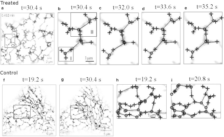
Illustration of the treated (top panels) and control (bottom panels) ER network and local dynamics. The rectangle Region O in panels a and f highlights a region with no cisternae. In control, panels f and g show a transition between the ER tubule and the cisternae in Region O. (b–e) Show details of the dynamics in Region O for treated and (h and i) show for control, with the geometric graphs (where plus-markers are persistent; o-markers are nonpersistent nodes; and lines are edges) abstracted from an image processing method as described in Image Processing Methods. Subregions I and II in panel b are used for modeling the dynamics of treated ER networks. The imaging data is taken from Sparkes et al. (9) (www.plantcell.org, Copyright American Society of Plant Biologists); dynamics in Region II is shown in Movie S1 and in control is shown in Movie S2, both found in the Supporting Material.

Euclidean Steiner networks

In this section, we introduce the notion of the Euclidean Steiner network (ESN), which is a slight generalization of a Steiner tree. To begin, we recall the definition of Steiner tree. A tree between a number of fixed points is a cycle-free connected graph having these points as its nodes, and a minimal spanning tree is a tree whose total length (sum of the lengths of all its lines) is as small as possible. However, one can often construct a shorter spanning tree between these fixed nodes u₁,u₂,⋅⋅⋅,u_p by including extra nodes x₁,x₂,⋅⋅⋅,x_M (26). By minimizing over the trees on extra points, local minima are called “Steiner trees” (ST), where the fixed nodes are called “terminals” and the additional points are called “Steiner points”, and the globally minimal is called the “Steiner minimal tree” (SMT). More precisely, a (Euclidean) ST is a tree whose length cannot be shortened by a small perturbation of Steiner points, even when splitting is allowed. By splitting a node v, one disconnects two or more of the lines at v and connects them instead to a Steiner point. There could be several STs between a set of terminals, and these differ in topology (i.e., a connection description specifying which pairs of points have a connecting line). Fig. 2, a and b, shows two STs with the same four terminals.

Figure 2.

Examples of STs (a and b) and ESNs with cycles (c and d); (bold dots) terminals; and (junctions between connecting lines) Steiner points. (a and b) Two STs for the same terminals. In all cases, the angles at Steiner points are 120° and the angles at terminals are at least 120°.

Consider a network G connecting a set of terminals and possibly additional points on the plane. We say G is an ESN between these terminals and the additional points are Steiner points, if no small perturbation of Steiner points will decrease the length, even if splitting is allowed. In contrast to an ST, an ESN can have cycles (see Fig. 2, c and d). Clearly, the shortest length ESN must be the SMT between terminals, and a cycle-free ESN is an ST. Analogous to STs (27), for ESNs all Steiner points are of degree-three (i.e., lines radiating outwards) and have angles 120° between edges, whereas the terminals must be of degree at most three and have angles not less than 120° between edges that meet there. Steiner points in STs and ESNs in this article are determined by GEOSTEINER (a software for computing Steiner trees; available from http://www.diku.dk/hjemmesider/ansatte/martinz/geosteiner/).

Image processing methods

We briefly outline the image processing method we use to dynamically extract the terminals and graphs from the sequence of two-dimensional imaging data of Sparkes et al. (9). The method is similar to that in Bouchekhima et al. (22); however, we distinguish between persistent and nonpersistent nodes. Persistent nodes, which are static over a give time duration, relate to the static nodes isolated by persistency mapping and are thought to be of biological significance in the ER structural organization (9). Thus, at a given time, the graph is composed of a number of persistent nodes {p₁,p₂,⋅⋅⋅,p_p} that are present in the given time duration and a number of nonpersistent nodes

$${\left\{s_i\right\}}_{i=1}^{k\left(t\right)+m\left(t\right)},$$

which is the union of the branching junctions

$${\left\{b_i\left(t\right)\right\}}_{i=1}^{k\left(t\right)},$$

and the degree-one nodes

$${\left\{o_i\left(t\right)\right\}}_{i=1}^{m\left(t\right)}.$$

Branching and/or degree-one nodes and their number may change during the remodeling of the ER.

The persistent nodes are found by

• 1.Taking average pixel intensities over a fixed time duration (we use a time duration 80 s of an entire movie as default unless otherwise stated),
• 2.Smoothing this averaged image by a Gaussian filter K_r,σ of kernel size r and standard variation σ, and
• 3.Finding the local maximum (using an 8-connected neighborhood) in the smoothed images after applying a threshold I₁.

We use the parameters r =3, σ = 0.08, and threshold I₁ = 110; the choice of these parameters is discussed in Section SA in the Supporting Material. See also the Supporting Material for Movie S1 and Movie S2.

To obtain the nonpersistent nodes, we smooth each image using the Gaussian filter K_r,σ followed by thresholding, with a threshold I₂ to give a binary image. We then find the skeleton (of one-pixel width and the same topology as the binary image) using a thinning algorithm (29). This gives nodes of nonpersistent degree-one (ends in the skeleton) and branching (junctions in the skeleton) that are not in the set of persistent nodes. We assume that the persistent nodes are always in the network by rounding the persistent nodes to the closest point on the skeleton. We use I₂ = 20 for the treated ER and I₂ = 35 for the control. The choice of these parameters is discussed in Section SA in the Supporting Material.

Because we are testing whether ER tubules are connected and conform to an ESN, we are focusing on a relatively simple region of the ER network, which is devoid of cisternae, with the long-term plan of extending the study to cover both morphological forms of the ER (tubules and cisternae). For the treated ER, we have studied the network within the Region O of Fig. 1 a. In this region, the nonpersistent nodes move and connect to other nodes within the region (see Fig. 1, b–d). For the control ER, due to its complex spatial dynamics as well as its rapid transition between tubular and cisternal forms (e.g., seen from Fig. 1, f and g), we choose different regions with no cisternae. We also choose different static images in the recording, such as Region O in Fig. 1 f, to study its network properties. In a chosen region, we take the largest connected component in the skeleton and the nodes on the skeleton. Each pair of nodes on the skeleton is connected by an edge if there is a path in the skeleton connecting the two nodes without passing other nodes. The length of each edge is given by the Euclidean distance between two nodes (i.e., the length of the line).

This process delivers a time-dependent sequence of geometric graphs G(t) = (V(t)), E(t)) between a set of persistent nodes V_p = {p_i} ⊂ V(t) that are static throughout the movie, a set of additional nonpersistent nodes V_s = {s_i(t)} ⊂ V(t) that vary in position and number, and a set of edges E(t) ={e_i(t)} that connect the nodes. Our image processing method gives ∼99.7% (95.3%) of pixels among the lines in the abstracted graphs for treated (control) ER networks agree with that in the binary images before skeletonization. This indicates that the ER filaments between nodes are well described by straight lines.

Results

We examine some properties of the instantaneous networks and test the hypothesis that they are close to ESNs, before looking at the dynamics of the networks for the treated and the control ER and biophysical properties of the ER networks.

Instantaneous ER networks

Fig. 3 a compares the number of nodes in the treated and control ER networks for the chosen regions, considering the population of graphs G(t) over all instants of time. The average number of total nodes in a given unit area are similar between treated and control ER. Moreover, in both networks, persistent nodes are mainly nonbranching (i.e., connecting one or two tubules), whereas nonpersistent nodes are mainly branching. However, the treated ER has a larger number of persistent nodes than nonpersistent nodes in a unit area, compared to the control ER, which has an approximately equal number of both. Comparing treated and control, the control ER has a larger number of nonpersistent nodes per unit area than the treated ER. These observations are in agreement with the dramatic dynamic changes seen in the control network versus the treated sample. In addition, the mean edge-length in the treated (1.34 ± 0.33 μm (N = 986)) and control (0.96 ± 0.013 μm (N = 2312)) ER networks is similar.

Figure 3.

Node and edge analysis of abstracted treated and control ER networks in chosen regions over the analyzed movies. (a) Number of persistent (left two bars) and nonpersistent (right two bars) nodes per unit area (10 μm²). The majority of persistent nodes are nonbranching; the majority of nonpersistent nodes are branching. In the treated ER, 77% are persistent nodes; however, in the control, the number of persistent and nonpersistent nodes are approximately equal. (b) Distribution of the number of edges from a nonpersistent node to nonpersistent nodes V_s (left) and to persistent nodes V_p (right).

Typically, nonbranching nodes (mainly persistent type) have one or two edges, and branching nodes (mainly nonpersistent type) have three edges for both treated and control ER nodes (a branching node will have fewer than three edges if it links with tubules that are extended outside the chosen region). To further clarify the linking structure between nodes, Fig. 3 b shows that for the treated ER networks, a majority (∼90%) of nonpersistent nodes are connected to three persistent nodes and no others, whereas for the control ER, the number of edges between different types of nodes is much more homogeneous. By contrast, Fig. S3 in the Supporting Material shows that the treated and control ER networks do not show significant difference in the distribution of the number of edges from a persistent node.

Fig. 4 (top) shows that the angles at nonpersistent nodes for both treated and control follow a normal distribution with a mean at ∼120° and a standard variation at ∼25°. Furthermore, a two-sample Kolmogorov-Smirnov test suggests that the two are from the same normal distribution. Fig. 4 (bottom) shows that angles of persistent nodes are predominantly larger than 120° for both treated and control ER. This agrees well with the hypothesis that the networks are perturbed ESNs, and that the nonpersistent branching nodes are perturbed Steiner points.

Figure 4.

Angle distribution for nonpersistent (top) and persistent (bottom) nodes for both treated (solid) and control (shaded) ER networks in chosen regions. The smooth curves show best Gaussian fits to the distribution from the corresponding treated (solid; with a mean 121.4° and standard variation 25.7) and control (shaded; with a mean 120.8° and standard variation 28.3) networks. For persistent nodes, 77.5% (69.2%) of angles are over 120° in treated (control) ER networks.

Moreover, Fig. 5 (and see Fig. S4, a and b) show examples of abstracted self-contained ER networks that are clearly close to an ESN whose terminals are the persistent and degree-one nodes. In particular, for the treated ER networks where terminals are consistent in the entire movie, we further show in Fig. S4, c and d, the distribution of branching nodes and the peaks of the distribution are close to Steiner points in the corresponding SMT. This also suggests that the instantaneous ER networks are well modeled as perturbed ESNs.

Figure 5.

The comparison of a control ER network (a) together with the abstracted geometric graph to the ESN (b) with terminals (circles) being the persistent and degree-one nodes from panel a. Nonpersistent nodes in panel a are not connected with nodes outside the region. The imaging data is taken from Sparkes et al. (9).

The treated ER network dynamics

We focus on the network dynamics observed in Region O in Fig. 1, where the region is chosen to be away from any cisternae of the ER. Because the persistent nodes are static, we can describe the network dynamics via movement of the nonpersistent nodes and changes of the network topology.

Instantaneous ER networks suggest that nonpersistent branching nodes can be thought of as Steiner points that reduce the total length of the graph. We thus propose a simple model for the dynamics of the graph using a Langevin equation to characterize the motion of nonpersistent nodes (ER junctions), x_i(t) ∈ R² (unit μm) for i = 1…M, as

$$\frac{d{x}_i}{dt}=-a{\nabla }_{x_i}f\left(x_i,\dots ,x_P\right)+\sqrt{2\sigma }\xi \left(t\right),$$ (1)

where f(x_i,…,x_p) represents the total length in the network between persistent and the given nonpersistent nodes (the network topology will be implicitly inferred from node locations). In the model, there is a drift coefficient a (unit μm/s) and a diffusion coefficient σ (unit μm²/s) modulating white noise ξ(t) with zero mean and autocorrelation 〈ξ(t) ξ(t′)〉 = δ(t − t′). A physical interpretation of these parameters is discussed in Estimation of ER Filament Tension and Cytoplasm Viscosity from the Model. In the following subsections, we examine the dynamics in the Regions I and II highlighted in Fig. 1 b.

Network dynamics in Region I

This region contains three persistent nodes and one nonpersistent node, and the topology between the nodes remains the same in the movie (see the Supporting Material), i.e., the nonpersistent node x is connected to three persistent nodes p_i ∈ R² for i = 1…3. In this case, the total network length is

$$f\left(x\right)=\sum _i|x-p_i|,$$

where |⋅| denotes the Euclidean norm in R² and the gradient is

$${\nabla }_{x}f\left(x\right)={\sum }_i\frac{x-p_i}{|x-p_i|}.$$

Using the method in Image Processing Methods, we obtain a time series x(nδ), n = 1,…,N for the positions of the nonpersistent node with a time step δ = 1.6 s. We estimate the diffusion coefficient σ ≈ 0.008 ± 0.001 μm²/s (N = 50) via quadratic variation (30) as

$$\sigma \approx \frac{1}{2Nd\delta }\sum _{n=1}^{N-1}|x\left(\left(n+1\right)\delta \right)-x\left(n\delta \right){|}^2,$$ (2)

where d = 2 is the dimension of the x and an asymptotically normal distribution for |x((n + 1)δ) – x(nδ)|² from Barndorff-Nielsen and Shephard (31) (see the Supporting Material for details). Meanwhile, we estimate the drift coefficient a ≈ 0.2 ± 0.04 μm/s (N = 50) by maximizing the approximated log-likelihood (32)

$$L_N\left(a\right)=\frac{1}{2\sigma }\left(-a\sum _{n=1}^{N-1}\langle \nabla f\left(x\left(n\right)\right),\left(x\left(n+1\right)-x\left(n\right)\right)\rangle -a^2\frac{\delta }{2}\sum _{n=1}^{N-1}\langle \nabla f\left(x\left(n\right)\right),\nabla f\left(x\left(n\right)\right)\rangle \right),$$ (3)

which gives

$$a=-\frac{{\sum }_{n=1}^{N-1}\langle \nabla f\left(x\left(n\right)\right),\left(x\left(n+1\right)-x\left(n\right)\right)\rangle }{{\sum }_{n=1}^{N-1}\delta |\nabla f\left(x\left(n\right)\right){|}^2}$$ (4)

and an asymptotically normal distribution for a from Newey and McFadden (33) (see the Supporting Material for details). Linearizing this Langevin equation (Eq. 1) gives a stochastic differential equation that models the dynamics of the nonpersistent node as a perturbed Steiner point, which can be solved analytically. The above estimations of the parameters in Eq. 1 agree well with the estimation on its linear part (see the Supporting Material for details).

The Langevin model with the estimated parameters well captures the ER dynamics in region I, through the comparison to the abstracted ER network dynamics in three different ways, as follows:

• 1.The angle distribution for the nonpersistent nodes,
• 2.The time-dependent total length f(x(t)), and
• 3.The position dynamics of the nonpersistent node x(t).

Indeed, the total length from a simulation of Eq. 1 oscillating above the length of the corresponding SMT is similar to that in the abstracted graphs (see top panels in Fig. 6). Meanwhile, Fig. S5 shows good agreement of numerical simulations for the positions and angles of nonpersistent nodes.

Figure 6.

Total length of abstracted graphs from experimental data, numerical simulation of the Langevin equation (Eq. 1) with an initial condition from the first frame, and the corresponding SMT in Region I (top) and II (bottom) highlighted in Fig 1b. (Right panel) Corresponding length distributions. The two sample Kolmogorov-Smirnov tests suggest the total length distribution calculated from experiment and simulation is from the same distribution in each region. Parameters σ = 0.008 μm²/s and a = 0.2 μm/s are used in simulations. Observe the periods of time between 20 and 45 s, where the topology flips to be close to an ST with a different topology in Region II.

Network dynamics in Region II

Region II in Fig. 1 b contains six persistent nodes, and more than one ST topology is possible (topology changes are not present in Region I). Possible connection structures between these nodes are shown in the top panel in Fig. 7, whereas the bottom panel in Fig. 7 shows four different STs corresponding to four observed ER network topologies. All STs with these six terminals have two Steiner points. The time-dependent length shown in Fig. 6 (bottom) illustrates that this length may oscillate about the (local) STs, but may also change between different ST topologies. Analogous to the dynamics in Region I, the positions of the nonpersistent nodes oscillate around the positions of Steiner points for the STs and the angles of nonpersistent nodes well fit a normal distribution with mean at ∼120° (see Fig. S6).

Figure 7.

(Top) Four different graph structures from a treated ER network at different times for Region II in Fig 1b. The p_i(i = 1, …, 6) indicate the locations of six persistent nodes, whereas x_1,2 indicate the locations of two nonpersistent nodes. (Bottom) Four STs correspond to the abstracted graphs shown above. (+) Persistent nodes, (○) nonpersistent nodes, and (□) Steiner points. The imaging data is taken from Sparkes et al. (9).

The transition between topologies may be associated with creation of additional nonpersistent nodes. Indeed, Fig. S7 indicates that such additional nodes can appear during transitions; this additional node in Region II only appears during two of the 50 frames in the recording. In modeling the dynamics in this region, we exclude these intermediate states and only model these four ST topologies in Fig. 7. More precisely, for the six persistent nodes {p_i=1}⁶, we simply assume rewiring occurs when one of the nonpersistent nodes crosses the lines $\overline{p_1{p}_2}$ or $\overline{p_4{p}_5}$ and the topology changes to be the closest to that in Fig. 7. We use the same parameters σ,a as in Region I to perform numerical solutions of the Langevin equation (Eq. 1). Fig. 6 (bottom) and Fig. S6 show that these simulations agree well with abstracted graphs in terms of the angle distribution for the nonpersistent nodes, the time-dependent total length, and the dynamics of nonpersistent nodes.

ER remodeling in the control

The previous section demonstrates that the treated ER network is well modeled as a perturbed ESN where the terminals correspond to the persistent nodes and perturbation is due to Brownian motion. The control ER network can also be viewed as a perturbed ESN as illustrated in Fig. 5 where terminals include persistent and degree-one nodes. However, the perturbation in the control is of higher amplitude and more heterogeneous than Brownian motion. The perturbations include Brownian forces, but streaming and organelle motion also have a major effect on the network structure. Indeed, the dynamics of the control ER network is much richer than that in the treated case, and we have not yet attempted to model the full dynamics of the control ER network even for the restricted regions. However, we do illustrate some of the challenges, and the complexity of the dynamics.

One problem in interpreting the dynamics of the control ER network is that some of the persistent nodes may only be visible for part of the sequence; there appear to be moments in which detachment/reattachment of the ER network occurs. This may lead to incorrect classification of persistent points or terminals as nonpersistent nodes. For example, Fig. 8 a show two nodes p_1,2 that only persistently appear for a proportion of the recording. This suggests that for the control ER network, persistent nodes can dynamically appear and disappear from the network.

Figure 8.

(a) The time-dependent maximal GFP intensity in a small neighborhood (with a radius distance of 3 pixels) indicating two persistent nodes p_1,2 that are only visible for part of the sequence. (b) Two consecutive networks at a chosen region in the native state illustrating examples of complex remodeling. (Thick rectangle) Region where loop closing occurs (branching also takes place); (thin rectangle) loop opening; (dashed rectangle) complex structural change that will presumably be resolved only by using a higher-time-resolution movie.

In the control sample, the ER network undergoes additional structural changes that can be much more complex than in the treated ER network. Phenomena such as node splitting to create additional degree-one nodes, opening and closing of loops, creation of new junctions, and destruction of nodes as well as edges (filaments), are all observed in the control. Fig. 8 illustrates some examples of these phenomenon in ER network remodeling.

Estimation of ER filament tension and cytoplasm viscosity from the model

We use the Langevin model Eq. 1 and the estimated parameters discussed in ER in The Treated ER Network Dynamics to obtain estimates for the ER filament tension force and the local effective viscosity, at least for the treated ER in Region I. The inertial forces involved are negligible and we make the following assumptions:

• A1.We suppose that the ER filaments are approximately cylindrical with constant radius R and surface tension γ, which means that the tension force F: = 2πRγ is approximately constant in the ER filaments.
• A2.We suppose that the environment outside the ER filament is fluid with constant effective viscosity η.
• A3.We suppose that the ER junction can be approximated as a sphere of radius R that is acted on purely by Stokes drag, filament tension, and Brownian forces.

For Region I and dynamics discussed in Network Dynamics in Region I, the nonpersistent node x(t) ∈ R² moves so that the tension and Stokes drag forces balance the Brownian forces; hence x(t) satisfies the Langevin equation

$$F{\nabla }_{x}f\left(x\right)+6\pi \eta R\frac{dx}{dt}=\sqrt{2k_{\text{B}}T6\pi \eta R}\xi \left(t\right),$$ (5)

where k_B is the Boltzmann’s constant and T is the temperature (34). This reduces to Eq. 1 with

$$\begin{array}{c}a=\frac{F}{6\pi \eta R}\text{,}\\ \sigma =\frac{k_{\text{B}}T}{6\pi \eta R}.\end{array}$$ (6)

The ER filament diameter is measured to be D = 2R = 0.06 μm (35) and the estimated diffusion coefficient σ ≈ 0.008 ± 0.001 μm² is comparable to ∼10⁻⁴ μm²/s measured for organelles of size ∼0.1 μm (36). Using T = 298 K, D = 2R = 0.06 μm and the estimated parameters a,σ from Network Dynamics in Region I, the relations in Eq. 6 gives an effective viscosity η and tension force F for the situation in Region I that are

$$\begin{array}{c}\eta \approx 909\pm 113.7\text{cP,}\\ F\approx 0.1\pm 0.02\text{pN,}\end{array}$$ (7)

where the error is from propagation of uncertainty (37) in drift and diffusion coefficients. However, Fig. 9 suggests that the time resolution means we are in the region of elastic behavior and the estimate of viscosity is overestimated. In particular, the mean-square displacement of the ER junction in Region I is almost independent of time lag; see Fig. 9 b. This suggests that the time resolution in the ER movie is in the region of elastic behavior and at this measured timescale, the cytoplasm behaves predominantly as elastic. Thus the effective viscosity η = 909 cP from Eq. 7 is merely an upper bound. It is well known that the cytoplasm displays both elastic and viscous characteristics (13,14), depending on the particle length scale in comparison to the cytoskeleton. For a smaller length scale, the interstitial liquid is only viscous, whereas for a larger length scale, as illustrated in Fig. 9 a, the cytoplasm is predominantly viscous at long timescales (t > t₂) and predominantly elastic at intermediate timescales (t₁ < t < t₂), and behaves again as a viscous liquid at timescales t < t₁.

Figure 9.

(a) Schematic graph for the mean-square displacement (MSD) of particles in a viscoelastic cytoplasm, which behaves as viscous liquid at long timescales (t > t₂), elastic solid at intermediate timescales (t₁ < t < t₂), and is viscous again at short timescales (t < t₁). (b) MSD of the nonpersistent node in Region I highlighted in Fig. 1b shows almost no dependence on time lags in a range of [1.6 s, 32 s] with an average of 0.0575 μm². (Bar) Error of the mean. The MSD of the node movement for a time lag t = kδ is approximated as ${\sum }_{n=1}^{N-k}|x\left(\left(n+k\right)\delta \right)-x\left(n\delta \right){|}^2/\left(N-k\right)$.

Discussion

Previous quantitative descriptions of ER network geometry have been restricted to fairly-rudimentary measures of filament length and static elements. ER network remodeling and the dynamic nature of this process have not been adequately described in a quantitative manner. Questions relating to whether all ER filaments are under constant tension and the filament formation is constrained, so that the entire network maintains a minimal length, remain unanswered. Understanding these basic principles provides a platform from which to determine and measure the effects of the molecular components controlling such events. Here, using experimental data from plants, we have shown that the ER network is constrained, and is well modeled as minimal networks that are perturbations of ESNs where the perturbations apparently involve random (Brownian) and deterministic (streaming and organelle motion) forces. The treated ER network is particularly amenable to this analysis in that the structure seems to be approximately constant over longer periods than for the control, and the network topology only changes locally.

This modeling approach has been validated by quantitative comparison of the dynamical networks extracted from the biological data, including the network length, displacement of junctions, and angle distributions of the junctions in the networks. This has enabled us to estimate the tension force of the ER network (and to a certain extent, the viscosity of the cytoplasm) simply from observing the sequences of images. Higher time- and space-resolution imaging should improve the accuracy of these estimates.

Many questions do remain unanswered, and we discuss a few of these below.

• 1.The mechanisms that regulate ER reorganization and remodeling are poorly understood. Better quantitative tools providing details on parameters relating to remodeling are required. Note that the distributions of the total length in Region I and Region II differ. Even in the treated condition, where ER dynamics are restricted (e.g., Fig. 7), the structural changes remain unclear, although additional branching points can transiently appear (e.g., Fig. S7). It would be particularly interesting to use higher temporal and spatial resolution imaging so that one can study, for example, the transitions between different topologies. A statistical model (e.g., for the total length of the network) would help quantify the network topologies, and large deviation theory could be used to quantify how often major topological changes are undergone by the network.
• 2.Several of the physical processes that determine the structure of the ER network in living cells are unclear. Our estimations of filament tension and viscosity, using Assumptions A1–A3, give a low diffusion coefficient (relatively high effective viscosity) and low tension force, compared to molecular motor stall forces or tether force, as estimated in Upadhyaya and Sheetz (12). A low tension force could be expected, because it allows dynamical remodeling of ER junctions under perturbations. However, the physical environment is much more complex. Both the vacuole and plasma membrane undergo dynamical surface alterations (local shape changes and deformation for vesicle exchange). The quasi-two-dimensional-like cytoplasmic region (which can also transverse the cell in trans-vacuolar strands that pierce and run through the vacuole) is packed with membrane-bound organelles, vesicles, protein complexes, cytoskeletal filaments, and macromolecules (such as carbohydrates). These substructures within the cytoplasm are not static, and appear to undergo seemingly random motion; the plant cytoplasm is known to be a highly heterogeneous environment, and Assumptions A1–A3 are likely to be challenged by further collection of data.
• 3.It may well be that tensions and filament diameter may vary around the network; nevertheless, assumption A1 could be experimentally explored in vitro and in vivo. Assumption A2 could be measured by comparing the fluctuations of shorter ER filaments if spatial resolution is increased to the point that these fluctuations can be resolved. Assumption A3 will be modified in the presence of other forces, for example by tethering forces to organelles or to the cytoskeleton, and it could be improved by more-detailed modeling of the membrane geometry at such junctions; however, this is likely to be computationally challenging. Detailed considerations of the motion of the filaments themselves (and not just the junctions) are likely to give a better but less tractable model.
• 4.Although the Langevin equation from Eq. 5 seems to model the treated ER dynamics well, it will be much harder to model the control ER dynamics without considerably more data at a higher spatial and temporal resolution. The remodeling discussed in ER Remodeling in the Control includes the extension/retraction of actin tubules and motion of organelles as well as interactions with regions of cytoplasmic streaming and drastic rearrangements of the entire ER. The topology can change substantially between frames, and this is not resolved, for example, in Movie S2 in the Supporting Material. This is evident from Fig. 8, where significant reorganization has taken place between two frames of the movie.

References

- 1.Levine T., Rabouille C. Endoplasmic reticulum: one continuous network compartmentalized by extrinsic cues. Curr. Opin. Cell Biol. 2005;17:362–368. doi: 10.1016/j.ceb.2005.06.005. [DOI] [PubMed] [Google Scholar]
- 2.Lynes E.M., Simmen T. Urban planning of the endoplasmic reticulum (ER): how diverse mechanisms segregate the many functions of the ER. Biochim. Biophys. Acta. 2011;1813:1893–1905. doi: 10.1016/j.bbamcr.2011.06.011. [DOI] [PMC free article] [PubMed] [Google Scholar]
- 3.Roussel B.D., Kruppa A.J., Marciniak S.J. Endoplasmic reticulum dysfunction in neurological disease. Lancet Neurol. 2013;12:105–118. doi: 10.1016/S1474-4422(12)70238-7. [DOI] [PubMed] [Google Scholar]
- 4.Viana R.J., Nunes A.F., Rodrigues C.M. Endoplasmic reticulum enrollment in Alzheimer’s disease. Mol. Neurobiol. 2012;46:522–534. doi: 10.1007/s12035-012-8301-x. [DOI] [PubMed] [Google Scholar]
- 5.Goyal U., Blackstone C. Untangling the web: mechanisms underlying ER network formation. Biochim. Biophys. Acta. 2013;1833:2492–2498. doi: 10.1016/j.bbamcr.2013.04.009. [DOI] [PMC free article] [PubMed] [Google Scholar]
- 6.Sparkes I., Hawes C., Frigerio L. FrontiERs: movers and shapers of the higher plant cortical endoplasmic reticulum. Curr. Opin. Plant Biol. 2011;14:658–665. doi: 10.1016/j.pbi.2011.07.006. [DOI] [PubMed] [Google Scholar]
- 7.Sparkes I.A., Ketelaar T., Hawes C. Grab a Golgi: laser trapping of Golgi bodies reveals in vivo interactions with the endoplasmic reticulum. Traffic. 2009;10:567–571. doi: 10.1111/j.1600-0854.2009.00891.x. [DOI] [PubMed] [Google Scholar]
- 8.Friedman J.R., Voeltz G.K. The ER in 3D: a multifunctional dynamic membrane network. Trends Cell Biol. 2011;21:709–717. doi: 10.1016/j.tcb.2011.07.004. [DOI] [PMC free article] [PubMed] [Google Scholar]
- 9.Sparkes I., Runions J., Griffing L. Movement and remodeling of the endoplasmic reticulum in nondividing cells of tobacco leaves. Plant Cell. 2009;21:3937–3949. doi: 10.1105/tpc.109.072249. [DOI] [PMC free article] [PubMed] [Google Scholar]
- 10.Griffing L.R., Gao H.T., Sparkes I. ER network dynamics are differentially controlled by myosins XI-K, XI-C, XI-E, XI-I, XI-1, and XI-2. Front. Plant Sci. 2014;5:218. doi: 10.3389/fpls.2014.00218. [DOI] [PMC free article] [PubMed] [Google Scholar]
- 11.Ueda H., Yokota E., Hara-Nishimura I. Myosin-dependent endoplasmic reticulum motility and F-actin organization in plant cells. Proc. Natl. Acad. Sci. USA. 2010;107:6894–6899. doi: 10.1073/pnas.0911482107. [DOI] [PMC free article] [PubMed] [Google Scholar]
- 12.Upadhyaya A., Sheetz M.P. Tension in tubulovesicular networks of Golgi and endoplasmic reticulum membranes. Biophys. J. 2004;86:2923–2928. doi: 10.1016/S0006-3495(04)74343-X. [DOI] [PMC free article] [PubMed] [Google Scholar]
- 13.Tseng Y., Kole T.P., Wirtz D. Micromechanical mapping of live cells by multiple-particle-tracking microrheology. Biophys. J. 2002;83:3162–3176. doi: 10.1016/S0006-3495(02)75319-8. [DOI] [PMC free article] [PubMed] [Google Scholar]
- 14.Wirtz D. Particle-tracking microrheology of living cells: principles and applications. Annu. Rev. Biophys. 2009;38:301–326. doi: 10.1146/annurev.biophys.050708.133724. [DOI] [PubMed] [Google Scholar]
- 15.Radochová B., Janáček J., Torori Z. Analysis of endoplasmic reticulum of tobacco cells using confocal microscopy. Image Anal. Stereol. 2005;24:181–185. [Google Scholar]
- 16.Puhka M., Vihinen H., Jokitalo E. Endoplasmic reticulum remains continuous and undergoes sheet-to-tubule transformation during cell division in mammalian cells. J. Cell Biol. 2007;179:895–909. doi: 10.1083/jcb.200705112. [DOI] [PMC free article] [PubMed] [Google Scholar]
- 17.Puhka M., Joensuu M., Jokitalo E. Progressive sheet-to-tubule transformation is a general mechanism for endoplasmic reticulum partitioning in dividing mammalian cells. Mol. Biol. Cell. 2012;23:2424–2432. doi: 10.1091/mbc.E10-12-0950. [DOI] [PMC free article] [PubMed] [Google Scholar]
- 18.West M., Zurek N., Voeltz G.K. A 3D analysis of yeast ER structure reveals how ER domains are organized by membrane curvature. J. Cell Biol. 2011;193:333–346. doi: 10.1083/jcb.201011039. [DOI] [PMC free article] [PubMed] [Google Scholar]
- 19.Griffing L.R. Networking in the endoplasmic reticulum. Biochem. Soc. Trans. 2010;38:747–753. doi: 10.1042/BST0380747. [DOI] [PubMed] [Google Scholar]
- 20.Sparkes I.A., Frigerio L., Hawes C. The plant endoplasmic reticulum: a cell-wide web. Biochem. J. 2009;423:145–155. doi: 10.1042/BJ20091113. [DOI] [PubMed] [Google Scholar]
- 21.Bouchekhima, A. N. 2009. Quantification of the Plant Endoplasmic Reticulum. Ph.D. thesis. University of Warwick, Coventry, UK.
- 22.Bouchekhima A.N., Frigerio L., Kirkilionis M. Geometric quantification of the plant endoplasmic reticulum. J. Microsc. 2009;234:158–172. doi: 10.1111/j.1365-2818.2009.03158.x. [DOI] [PubMed] [Google Scholar]
- 23.Park S.H., Blackstone C. Further assembly required: construction and dynamics of the endoplasmic reticulum network. EMBO Rep. 2010;11:515–521. doi: 10.1038/embor.2010.92. [DOI] [PMC free article] [PubMed] [Google Scholar]
- 24.Fomenko A.T. Gordon & Breach; Williston, VT: 1989. The Plateau Problem: Historical Survey. [Google Scholar]
- 25.Terasaki M., Shemesh T., Kozlov M.M. Stacked endoplasmic reticulum sheets are connected by helicoidal membrane motifs. Cell. 2013;154:285–296. doi: 10.1016/j.cell.2013.06.031. [DOI] [PMC free article] [PubMed] [Google Scholar]
- 26.Courant R., Robbins H. Oxford University Press; New York: 1941. What Is Mathematics? [Google Scholar]
- 27.Hwang F.K., Richards D.S., Winter P. Vol. 53. Elsevier Science Publishers; North-Holland, Amsterdam, The Netherlands: 1992. The Steiner tree problem. (Annals of Discrete Mathematics). [Google Scholar]
- 28.Reference deleted in proof.
- 29.Guo Z., Hall R.W. Parallel thinning with two-subiteration algorithms. Commun. ACM. 1989;32:359–373. [Google Scholar]
- 30.Øsendal B. 5th Ed. Springer-Verlag; Berlin, Germany: 1998. Stochastic Differential Equations: An Introduction with Applications. [Google Scholar]
- 31.Barndorff-Nielsen O.L.E.E., Shephard N. Realized power variation and stochastic volatility models. Bernoulli. 2003;9:243–265. [Google Scholar]
- 32.Yoshida N. Estimation for diffusion processes from discrete observation. J. Multivar. Anal. 1992;41:220–242. [Google Scholar]
- 33.Newey W.K., McFadden D. Chapter 35: Large sample estimation and hypothesis testing. In: Engle R., McFadden D., editors. Vol. 4. Elsevier; North-Holland, Dordrecht, The Netherlands: 1994. (Handbook of Econometrics). [Google Scholar]
- 34.Coffey W.T., Kalmykov Y.P., Waldron J.T. Vol. 14. World Scientific Publishing Company; Singapore: 2004. (The Langevin Equation: With Applications to Stochastic Problems in Physics, Chemistry and Electrical Engineering, 2nd Ed. World Scientific Series in Contemporary Chemical Physics). [Google Scholar]
- 35.Shibata Y., Hu J., Rapoport T.A. Mechanisms shaping the membranes of cellular organelles. Annu. Rev. Cell Dev. Biol. 2009;25:329–354. doi: 10.1146/annurev.cellbio.042308.113324. [DOI] [PubMed] [Google Scholar]
- 36.Manneville J.B., Etienne-Manneville S., Ferenczi M. Interaction of the actin cytoskeleton with microtubules regulates secretory organelle movement near the plasma membrane in human endothelial cells. J. Cell Sci. 2003;116:3927–3938. doi: 10.1242/jcs.00672. [DOI] [PubMed] [Google Scholar]
- 37.Taylor J.R. 2nd Ed. University Science Books; Sausalito, CA: 1997. An Introduction to Error Analysis: The Study of Uncertainties in Physical Measurements. [Google Scholar]
Associated Data
This section collects any data citations, data availability statements, or supplementary materials included in this article.