Environmental Safety of the Use of Major Surfactant Classes in North America

Abstract

This paper brings together over 250 published and unpublished studies on the environmental properties, fate, and toxicity of the four major, high-volume surfactant classes and relevant feedstocks. The surfactants and feedstocks covered include alcohol sulfate or alcohol sulfate (AS), alcohol ethoxysulfate (AES), linear alkylbenzene sulfonate (LAS), alcohol ethoxylate (AE), and long-chain alcohol (LCOH). These chemicals are used in a wide range of personal care and cleaning products. To date, this is the most comprehensive report on these substance's chemical structures, use, and volume information, physical/chemical properties, environmental fate properties such as biodegradation and sorption, monitoring studies through sewers, wastewater treatment plants and eventual release to the environment, aquatic and sediment toxicity, and bioaccumulation information. These data are used to illustrate the process for conducting both prospective and retrospective risk assessments for large-volume chemicals and categories of chemicals with wide dispersive use. Prospective risk assessments of AS, AES, AE, LAS, and LCOH demonstrate that these substances, although used in very high volume and widely released to the aquatic environment, have no adverse impact on the aquatic or sediment environments at current levels of use. The retrospective risk assessments of these same substances have clearly demonstrated that the conclusions of the prospective risk assessments are valid and confirm that these substances do not pose a risk to the aquatic or sediment environments. This paper also highlights the many years of research that the surfactant and cleaning products industry has supported, as part of their environmental sustainability commitment, to improve environmental tools, approaches, and develop innovative methods appropriate to address environmental properties of personal care and cleaning product chemicals, many of which have become approved international standard methods.

I. INTRODUCTION

Since the late 1930s and early 1940s when the first synthetic surfactants were developed, surfactants have been increasingly used as the active ingredient in a wide variety of consumer products such as personal care products (e.g., shampoos, body wash) and in household cleaning products (e.g., dishwashing detergents, laundry detergents, hard-surface cleaners). Detergents that contained these surfactants increased in popularity because these provided better cleaning and more suds than traditional soaps and at lower prices. By 1953, in North America, the number of pounds of detergent products containing synthetic surfactant sold exceeded that of soaps. This rapid expansion of synthetic detergents led to environmental challenges as the wastewater was discharged into surface waters. In the late 1940s, foaming in streams and at wastewater treatment plants (WWTPs) were first reported, and by the early 1950s scientific evidence identified the cause as synthetic surfactants, especially alkyl benzene sulfonates (ABS), the most widely used surfactant, because it was not readily biodegradable (Sallee et al., 1956).

The observation of environmental effects resulted in the commitment in 1951 by the Association of American Soap and Glycerine Producers (founded in 1926), predecessor to The Soap and Detergent Association (SDA or Association), which was formed in 1962, and its members, to study and understand the environmental fate and effects from synthetic surfactant usage and to search for replacements that would not result in unacceptable adverse impacts on the surface waters. For example, in 1965, U.S. detergent manufacturers voluntarily switched from ABS to linear alkylbenzene sulfonate (LAS), which had the same cleaning performance characteristics but was more readily biodegradable (Hanna et al., 1964a, 1964b). Within a few years the number of foaming incidents had dropped, and the concentration of surfactants in the nation's waterways had been reduced (Coughlin, 1965).

Since this initial environmental research in the 1950s, the Association, now named the American Cleaning Institute® (the Institute) (ACI), has been conducting environmental research on cleaning product ingredients, including synthetic surfactants. It also has committed to publication of the results of this research in the open literature. In fact, the first environmental publication of the SDA entitled Synthetic Detergents in Perspective was published in 1962 (The Soap and Detergent Association [SDA], 1962). In the 1970s and early 1980s, the SDA issued critical reviews of human and environmental safety data of major surfactants (SDA, 1977, 1981), which summarized the data and the understanding of the risk to the environment based on the data that had been collected. These were updated in 1991 (SDA, 1991a, 1991b, 1991c).

The Institute has continued to conduct environmental research on these surfactants as a component of its environmental sustainability commitment: “To only market products that have been shown to be safe for humans and the environment, through careful consideration of the potential health and environmental effects, exposures and releases that will be associated with their production, transportation, use, and disposal.” Because it has been over 20 years since the environmental research was summarized, the purpose of this review is to summarize new data and findings and to update the understanding of the environmental risks of surfactants currently used in consumer and commercial products. Moreover, SDA, ACI, and the Council for LAB/LAS Environmental Research (CLER) has participated both in the voluntary national United States Environmental Protection Agency (U.S. EPA) right-to-know program for High Production Volume (HPV) chemicals as well as the voluntary global International Council of Chemical Associations (ICCA) HPV chemicals program and thereby collected significant data set on the environmental health and safety of several major classes of surfactants.

ACI and its member companies have spent no less than 30 million USD on the assessment and reporting of the environmental safety of the major surfactants over the past 5 decades in ACI and its predecessor association's activities. The projects span the development of analytical, modeling, and sampling methods, as well as fate, effects, and monitoring studies. Well over 250 peer-reviewed and publicly available papers and reports have been published due to the efforts of ACI, its predecessor associations and its member companies; over 70 are available at http://www.aciscience.org/free of charge.

The review will cover the fate, exposure, and ecotoxicity effects of these surfactants to the aquatic and sediment environments. In addition, the aquatic and sediment risk will be evaluated using both prospective, i.e., based on modeling prediction, and retrospective, i.e., based on field monitoring data, analysis as well as key learnings developed as a result of this additional research. The focus of this review will be on the major synthetic surfactants which account for over 72% of the surfactants used in North America, which includes U.S. and Canada (i.e., alcohol ethoxylates (AE), alcohol sulfates (AS), alkyl ethoxysulfates (AES), and linear alkylbenzyne sulfonate (LAS) (Colin A. Houston & Associates, Inc., 2002)). In addition the long-chain alcohols (LCOHs), which are not surfactants or used as such per se, are discussed because these are a very important feedstock to consider when discussing this suite of alcohol-based surfactants. In this paper, the LCOHs are included within the general term, surfactants.

The aim of this paper is fourfold:

• 1)To concisely report all the most relevant environmental data generated regarding surfactants over the recent decades in a single review paper;
• 2)To demonstrate the advancement and increased understanding of the risk assessment of surfactants, as well as how to conduct risk assessments for categories of compounds;
• 3)Provide an overview of the key scientific findings;
• 4)Finally, to reaffirm the industry's sustainability commitment and commitment to transparency and scientific advancement.

II. SURFACTANT OVERVIEW

Surfactants are organic compounds that contain both hydrophobic groups (their “tails”) and hydrophilic groups (their “heads”) making them soluble in both organic solvents and water. The hydrophobic group in a surfactant consists of an 8–18 carbon hydrocarbon, which can be aliphatic, aromatic, or a mixture of both. Surfactants in which the hydrocarbon is sourced from biological oils or fats such as palm oil or tallow are known as oleo-chemicals. Surfactants in which the source of the hydrocarbon is petroleum or gas are known as petrochemicals. In addition to the source of the hydrocarbon, surfactants are classified into nonionic, anionic, cationic, or zwitterionic by the presence or absence of formally charged hydrophilic head groups. The most widely used type of surfactants are anionic surfactants, such as LAS, AS, and AES, which are used for laundering, dishwashing detergents and shampoos because of their excellent cleaning properties and high sudsing potential. Another high volume surfactant is the nonionic surfactant, AE. Most laundry detergents contain both nonionic and anionic surfactants because nonionic surfactants contribute to making the surfactant system less sensitive to water hardness. The volume of cationic and zwitterionic surfactants is much lower, and thus they will not be addressed in this paper which focuses on the highest volume surfactants. The end use of these high volume surfactants is in laundry detergents, dishwashing detergents, household cleaners, and personal care products both in the home, industrial, and institutional applications. These applications will result in release to the environment, primarily in wastewater discharges.

The choice of feedstock (e.g., oleochemical or petrochemical) typically depends on the relative cost and availability of raw materials needed to make the hydrocarbon tail of the surfactant, which is typically a detergent range fatty alcohol. Because of fluctuations in both price and accessibility to raw materials, the ratio of feedstock used is variable. Since three of these surfactants (i.e., AE, AES, and AS) are based on adding a hydrophilic group to a fatty alcohol, these three major surfactants are often related to each other as shown in Figure 1 and Table 1. As will be discussed in Section II.E.2, the manufacturing route of LAS is different from these three surfactants; therefore, it is not included in Figure 1.

FIGURE 1.

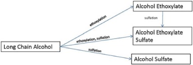
Production scheme for major surfactants.

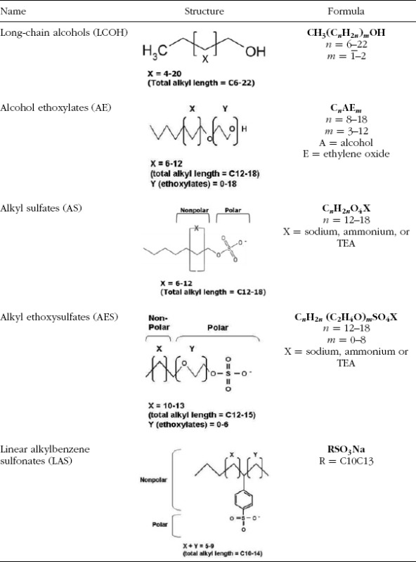
TABLE 1.

Chemical structure

Because all these surfactants, AE, AS, AES, and LAS and the feedstock, LCOH, are used in a wide variety of consumer products such as laundry detergents, dishwashing detergents, and shampoos, these surfactants are considered HPV chemicals. The consumption of each of the major surfactants and detergent alcohols from 1990 to 2008 in North America (US and Canada) is provided in Figure 2 (SRI Consulting, 2009a, 2009b). The 2008 data, which are the most recent reporting, also include consumption in Mexico. The total consumption volume of these surfactants ranges from 719,000 metric tons in 1990 to 895,500 metric tons in 2004 with an average over these years of approximately 787,000 metric tons.

FIGURE 2.

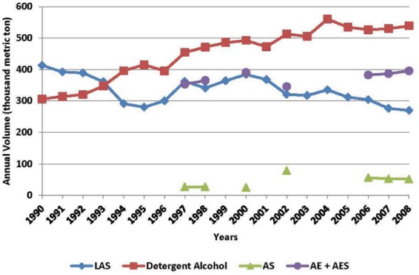
Annual consumption in North America of the different classes of surfactants.

A. Long-Chain Alcohols

Long-chain, or fatty, alcohols are not surfactants or used as such per se. However, these are very important to consider when discussing the suite of alcohol-based surfactants in this review. As illustrated in Figure 1, LCOHs are used as starting blocks for the synthesis of nonionic AE, and anionic AS and alcohol ethoxysulfates (AES). Furthermore, alcohols are found as minor components of commercial AE, AS, and AES, as a degradation product of these surfactants in the environment, and from natural biosynthesis (Mudge et al., 2008).

1. Chemical Structure

The alkyl chain length of LCOH (Table 1) was identified by the OECD HPV program to range from C₆ to C₂₂ (The Organisation for Economic Co-operation and Development [OECD], 2006); however, the typical range in detergents of interest is between C₉ to C₁₈ as verified in several monitoring programs for alcohol and alcohol-based surfactants (Mudge et al., 2008, 2010, 2012; Mudge, 2012). The alcohol group is usually located in the terminal position of the aliphatic chain, but not necessarily so, and are normally saturated (no double bonds).

2. Manufacture Route

Long-chain, or fatty, alcohols are sourced both from plant or animal oils and fats, as well as chemically modified or synthesized from petroleum. Alcohols used in detergents are most commonly between 12 and 18 carbons in length and are classified by the source of raw materials used to produce them. Oleochemical alcohols are derived from biological fats and oils whereas petrochemical alcohols are derived from crude oil, natural gas, gas liquids, or coal.

In living organisms, long-chain hydrocarbons are usually synthesized in the form of triacylglycerol. The feedstocks for oleochemicals are derived from these plant or animal hydrocarbon oils by separating out the triglycerides and chemically converting them into alcohol intermediates (Mudge et al., 2008). Tallow from animal fat, palm, palm kernel, and coconut oils are common sources for detergent alcohol production. Triglycerides of biological origin can also be chemically modified through hydrolysis to yield fatty acids and glycerol. For example, methanol can also be used to transesterify triglycerides yielding fatty acid methyl esters and glycerol which can be subsequently used in other applications. Oleochemical fatty alcohols are then produced by hydrogenation of the fatty acid methyl esters and fatty acids.

Petrochemical fatty alcohols are derived using linear hydrocarbon chains or normal paraffin extracted from petroleum. Kerosene and gas oil contain the hydrocarbon chain lengths of greatest interest and are frequently used as precursors for the manufacture of alcohols. A variety of interesting industrial processes have been devised to produce petrochemical fatty alcohols, including the Ziegler ethylene growth production process to form Ziegler alcohols, conventional oxo-alcohols using internal olefins, the SHOP (Shell Higher Olefin Process) for modified oxo-alcohols, and production of oxo-alcohols from Fischer–Tropsch alpha-olefins (Mudge et al., 2008). Collectively, these methods are used to produce a wide range of mid to high carbon chain length alcohols with single to minimal mono-methyl branching, all of which find their way into detergent manufacture.

3. Use and Volume Information

Alcohols are broadly used in detergent, pharmaceutical, and plastics industry (see Mudge et al. (2008) for a comprehensive review). The estimated North American production volume of these LCOHs based on a 2002 survey was 624,261 metric tons (OECD, 2006). Based on a global survey (OECD, 2006), approximately 50% of this total production volume is used directly in final products with the remainder used as an intermediate for production of other chemicals. Approximately 65% of the volume used as intermediates are produced and consumed on-site, primarily in the production of surfactants. A subset of these LCOHs, which is most commonly used as intermediates in surfactant production, contain 12 or more carbon atoms in chains that are >35% linear.

North American production of detergent alcohols ranged from 494,200 metric tons in 1999 to 381,000 metric tons in 2008. Production is expected to increase annually by 2.5% after this decline of 2.7% from 2003 to 2008 (SRI Consulting, 2009a). This volume not only represents mostly C₁₂–C₁₆ alcohols with a high degree of linearity but also includes some C₁₆–C₂₀₊ alcohols which are used mainly in personal care products and oilfield markets. Over 99% of detergent alcohols produced in North America are in the C₁₂–C₁₈ range, while the balance consists of products containing 20 or more carbon atoms (SRI Consulting, 2009a). All of the North American detergent alcohol production is located in the United States.

While the North American production of these detergent alcohols has been decreasing in recent years, the demand has been increasing. For example, the 2009 North American demand for these detergent alcohols is estimated to be 535,000 metric tons with 356,400 metric tons produced in North America, and the remainder coming from imports (SRI Consulting, 2009a). North American consumption is projected to increase annually by 1.9% from 2008 to 2013 which is in line with past increases annually of 1.3% from 2003 to 2008 and 1.6% from 1997 to 2003.

The bulk of the surfactants produced from the detergent alcohols go into household detergents, followed by personal care applications (SRI Consulting, 2009a). AEs (41.6% worldwide), AS (13.2% worldwide), and alcohol ether sulfates (27.6% worldwide) accounted for 82.4% of worldwide detergent alcohol demand in 2008. Less than 6% of the production was used as free alcohols in 2008. Most of these free alcohol applications exploit their lubricating, emollient, solubilizing, or emulsifying properties. The total North America consumption of free alcohols (C₁₂–C₁₈ range) in 2008 was estimated at 29,000 metric tons (SRI Consulting, 2009a). It is estimated that 22.5 thousand metric tons of this 29,000 metric tons are used in cosmetics, mainly as solvents, emollients, and conditioners. Consumption of free alcohols in these applications is expected to grow at an average annual rate of 2.3% from 2008 to 2013.

4. Physical and Chemical Properties

An extensive data set of physical and chemical properties of LCOHs is described in peer-reviewed Screening Information Data Set (SIDS) documentation and discussed in the SIDS Initial Assessment Report (SIAR) (OECD, 2006). These data are summarized in Fisk et al. (2009) and Schäfers et al. (2009). Furthermore Fisk et al. (2009) provide a comparison of the measured physicochemical properties and those predicted using quantitative structure activity relationships (QSARs), specifically those contained in EPISuite 3.12 (http://www.epa.gov/oppt/exposure/pubs/episuite.htm). The chemical properties of alcohols are directly related to the length of the aliphatic, or hydrophobic, chain (Table 2). Fisk et al. (2009) demonstrate that solubility and vapor pressure of alcohols decrease with increasing chain length. With increasing chain length, hydrophobicity increases as does melting and boiling point. Since these properties of pure alcohol compounds follow these predictable trends, these are amenable to estimation by QSAR. For most of the physicochemical properties, as demonstrated in Fisk et al. (2009), the EPISuite 3.12 models predicted the properties very well. However, for the longer carbon length chains, where the log K_ow predictions were >6, an overprediction was observed that was easily corrected by including a term based on carbon number. These QSAR models can in turn be used to provide a rational understanding of the way that the multicomponent commercial products behave and consequently to predict the environmental behavior and ecotoxicity of these commercial substances.

TABLE 2.

Physical and chemical data for long-chain alcohols

Alcohol	Carbon length	Melting point (°C)	Boiling point (°C)	Vapor pressure (Pa) at 25°C	Kow	Water solubility (mg/L)
1-Hexanol	6	−50.0	145–170	122.00	2.03	5900
1-Octanol	8	−16.0	194–195	10.00	3.15	551
1-Decanol	10	6.4	220–240	1.13	4.57	39.5
1-Undecanol	11	14.0	245	3.90 × 10−1	4.72	8
1-Dodecanol	12	24.0	259	1.13 × 10−1	5.13	1.9
1-Tridecanol	13	32.0	276	5.70 × 10−2	5.51	0.38
1-Tetradecanol	14	40.0	289	1.40 × 10−2	6.03	0.191
1-Pentadecanol	15	45.0	318*	5.12 × 10−3	6.43	0.102
1-Hexadecanol	16	50.0	334–344	1.40 × 10−3	6.65	0.013
9-Octadecen-1-ol	18	17.0	333	1.98 × 10−3	7.07	0.0077
1-Eicosanol	20	66.0	309	1.50 × 10−5	7.75	0.0027
1-Docosanol	22	72.5	401	8.15 × 10−6	7.75	0.0027

^*One value is estimated, all others are measured (from SIAR 2002, 2006).

Sources: Sanderson et al. (2009); Fisk et al. (2009); OECD (2002, 2006); Estimation Program Interface for Windows (EPIWIN) (Suite v. 4.1) software.

5. Environmental Fate Properties

Biodegradation. Numerous biodegradation studies have been performed for LCOHs (OECD, 2006). Results from the OECD 301 Ready Biodegradability test indicate that LCOHs with carbon chain lengths less than C₁₆ are Readily Biodegradable reaching >60% CO₂ evolution within the 10-day window (OECD, 2006). The C_16–18 alcohols achieve >60% CO₂ evolution over the 28-day test period but not always within the 10-day window and thus are considered Inherently Biodegradable (OECD, 2006). The alcohols with chain lengths greater than C₁₈ degrade at a much slower rate (e.g., 37% CO₂ evolution for C₁₈ over the 28-day test (OECD, 2006; Fisk et al., 2009). However, a recent publication demonstrates that alcohols up to C22 meet the criteria of readily biodegradable (Federle, 2009).

In a more definitive study, Federle and Itrich (2006) evaluated the biodegradation of LCOHs in activated sludge using radiolabeled (¹⁴C) C₁₂, C₁₄, and C₁₆ alcohols. Because of the use of radiolabeled material, the alcohols were dosed at more environmentally realistic concentrations when compared to the OECD 301 Ready Biodegradability test (10 μg/L versus 10 mg/L). After a 48-hr incubation period, there was 74% CO₂ evolution for C₁₂ alcohol, 77% CO₂ evolution for C₁₄ alcohol, and 65% CO₂ evolution for C₁₆ alcohol. Corresponding first-order loss rates of the parent compounds were 113 hr⁻¹ for C₁₂ alcohol, 87 hr⁻¹ for C₁₄ alcohol, and 103 hr⁻¹ for C₁₆ alcohol. These results illustrate that C_12–16 alcohols rapidly biodegrade in activated sludge with half-lives on the order of minutes.

The anaerobic biodegradation of LCOHs has also been investigated. Alcohols with chain lengths of C₈, C₁₆, and C_16–18 rapidly biodegrade under anaerobic conditions with gas production (CO₂ and CH₄), ranging from 75% to 95% over a 4–8 week test period (Shelton and Tiedje, 1984; Steber and Wierich, 1987; Steber et al., 1995; Nuck and Federle, 1996). These results further support the ready biodegradability of LCOH when the carbon chain is less than or equal to C₁₈.

Sorption. Sorption distribution (K_d) coefficients for several LCOHs (C₁₂, C₁₄, C₁₆, and C₁₈) to activated sludge and river water solids were determined by van Compernolle et al. (2006). The measured K_d values were 3,000 L/kg for C₁₂ alcohol, 8,490 L/kg for C₁₄ alcohol, 23,800 L/kg for C₁₆ alcohol, and 78,700 L/kg for C₁₈ alcohol. These results illustrate that LCOHs are highly sorptive to activated sludge and river water solids, particularly the C₁₆ and C₁₈ chain length alcohols. Based on these data, Fisk et al. (2009) developed the following QSAR for LCOHs.

log K_d = 0.642 + 0.235 × (chain length) (R² = 0.99, n = 4)

This relationship illustrates that alcohol sorption is proportional to the alkyl chain length, which in turn decreases the bioavailable fraction in aquatic environments as the alkyl chain length increases. This model has been used to adjust exposure concentrations of LCOH for bioavailability in aquatic risk assessments (Belanger et al., 2009).

B. Alkylethoxylates

1. Chemical Structure

The alkylethoxylate surfactants are defined by the basic structure C_x–yE_n, where the subscript following the “C” indicates the range of carbon chain units, and the subscript to the “E” indicates the average number of ethylene oxide (EO) units. EO indicates the average number of ethylene oxide (EO) units (Table 1). Note that EO is also often referred to as ethoxylate and ethoxylate number.

2. Manufacture Route

Alkylethoxylate surfactants are primarily produced from linear and essentially linear detergent alcohols (Figure 1) and to a lesser extent from linear random secondary alcohols from oleochemical or petrochemical feedstocks by ethoxylation with EO, using base-catalyzed reaction with potassium or sodium hydroxide followed by neutralization with an acid such as acetic or phosphoric acid. Alkylethoxylates commonly used in household products have carbon chains ranging between C₈ to C₁₈ and average EO chain lengths between 3 and 12 units (Human and Environmental Risk Assessments [HERA], 2009b).

The degree of branching and saturation, and the chain length distribution of the commercial AE will vary by the feedstock source and by the method used to produce the alcohols. The sources of the linear alcohols used in the manufacture of AEs are oleochemical or petrochemical feedstocks (OECD, 2006; Mudge et al., 2008). These alcohols can be produced as single carbon fractionations, but more commonly are produced as wider fractionations from within the range C₆ through C₂₂. Some alcohols derived from oleochemical sources will be mixtures of saturated, primary linear aliphatic alcohols and their saturated, mono-branched primary alcohol isomers but may also contain unsaturated primary non-branched-aliphatic alcohols (OECD, 2006). Furthermore, alcohols derived from oleochemical sources via the so-called “oxo-chemistry” may fall in the range C₇–C₁₇ and contain even- and odd-numbered carbon chains. The proportion of linear alcohols in these mixtures ranges from 90% to around 50% (OECD, 2006). This subcategory also contains a closely related mixture of saturated C₁₂–C₁₃ primary alcohols derived from Fischer–Tropsch olefins consisting of approximately 50% linear, 30% mono-methyl branched, and 20% other unintended components. This product is referred to as C10–16 alcohols Type B [CAS 67762-41-8] (OECD, 2006). Essentially linear alcohols, also known as oxo-alcohols, are produced from primary alcohols derived from branched butylene oligomers. A small amount (<5%) of the AEs used in household applications have a greater than mono degree of branching. This wide range of alcohols is substantially interchangeable as precursors for AE production.

Most of the commercial AE produced is shipped in either solid, paste, or solution form. The commercial product may also contain some reaction by-products such as unreacted alcohol, which is typically present between 2% and 42% with the average concentration being approximately 13% (Shell Chemicals LP, website document on Neodol^TM).

3. Use and Volume Information

A large portion of the AE surfactants manufactured in North America are converted to AES surfactants. In 2008, about 58% of the AE in North America was converted to AES (SRI Consulting, 2009a). The primary use of the remaining AE is in laundry detergents. To a lesser extent, according to SRI Consulting (2009a), AE is used in hand dish detergents, in personal care products such as shampoos, liquid hand soaps, and body washes, and in household, institutional, and industrial cleaners. Finally, AE is used in industrial processes within agriculture, textile, paper, and oil industries (SRI Consulting, 2009a; HERA, 2009b).

In 2008, about 395.4 thousand metric tons of detergent alcohols in North America were used in the production of AE. In 2008, about 58% of the AE was converted to AES. Thus, the volume of AE produced in 2008 was 166,070 metric tons. The use of AE in laundry liquids continues to grow as the use of these products continues to increase. The very strong growth in AE production and consumption in the 1980s and 1990s was driven by the strong growth in sales of laundry liquids. About 11% of the AE produced in 2008 was used in household hand dishwashing liquids; however it is difficult to determine exactly how much AE was used in this application because AE is generally not employed at high levels in these hand liquid detergents because it produces excess dryness and irritation, instead, the much milder AES or AS are used as the major surfactant in these products (SRI Consulting, 2009a). About 10% of the use of AE in 2008 was in personal care products, largely shampoos, liquid hand soaps, and body washes. The latter two product types have been growing in recent years as replacements for bar soaps that are largely based on sodium salts of fatty acids. About 5% of AE and AES consumption in 2008 is accounted for by several newly introduced or reformulated household hard-surface cleaners (SRI Consulting, 2009a). Very low levels of specialty AE are used as emulsifiers in cleansing creams and a few other personal care products. However, as in dishwashing liquids, other milder surfactants are used at much higher levels than AE to offset any adverse effects of AE on the skin. Non-household applications, such as industrial, institutional, and commercial cleaning products, accounted for 12% of AE consumption in 2008. About 10% of AE production was exported from North America in 2008.

4. Physical and Chemical Properties

Because AE surfactants are composed of compounds that differ in the number of carbon units and the number of EO units, the physicochemical properties of AE surfactants span a broad range. Although very little specific information is available concerning several of the physicochemical properties of specific AE homologues, an extensive data set is available for the alcohols (the EO = 0 homologues), as discussed in Section II.A.4. These data are used to set upper or lower limits for the specific physicochemical property for the other AE homologues (HERA, 2009b). The most important of the physicochemical properties over a range of alkyl chain length and ethoxylate number are summarized in Table 3.

TABLE 3.

Physical and chemical data for AE

Carbon length	EO	Melting point (°C)	EO	Boiling point (°C)	EO	Kow	EO	Water solubility (mg/L) solubility (mg/L)
8	0	−15.5 to −17	0	194–195 (ambient)	0–22	Decreases with increasing EO from 3.03 to 0.97	0	551
9					0–22	Decreases with increasing EO from 3.57 to 1.51
10	0	6.4	0	229 (ambient)	0–22	Decreases with increasing EO from 4.11 to 2.05	0	39.5
	6	16.7	2	100 (0.4 mmHg)			8	510
	7	20.0–20.1	3	145 (0.48 mmHg)
	8	25.8–26	4	173 (0.2 mmHg)
			5	183 (0.15 mmHg)
			6	230 (0.5 mmHg), 200 (0.02 mmHg)
11					0–22	Decreases with increasing EO from 4.65 to 2.59
12	0	22.6–24	0	255–269 (ambient)	0–22	Decreases with increasing EO from 5.19 to 3.13	0	1.93
	2	18.0–18.2	2	175–180 (3.0 mmHg)			2	75 (linear C12–14)
	5	23.6–24.0	3	204–212 (6.0 mmHg)			3	11 (linear C12–14)
	6	25.0–25.7	4	235–245 (3.0–4.0 mmHg), 152 (0.01 mmHg)
			5	26.4
	8	30.0–31.0	5	202–216 (0.5 mmHg)			6	30.6
			6	205 (12 mmHg)			7	34.1
			8	232 (0.01 mmHg)			8	38.2
			12	281 (0.1 mmHg)			9	18 (linear C12–14)
13	0	30.6 or 32–33	0	276 (ambient)	0–22	Decreases with increasing EO from 5.73 to 3.67	0–40	Increases with increasing EO from 0.38 to 1000 (branched)
14	0	39–40	0	289 (ambient)	0–22	Decreases with increasing EO from 6.27 to 4.21	0	0.191
	2	28–29	2	174–176 (1.5 mmHg)			2	75 (linear C12–14)
	3	25.7–27	3	181–184 (0.5 mmHg)			3	11 (linear C12–14)
	4	28.5–29.5	4	204–206 (0.55 mmHg)			6	12 (linear C12–14)
	5	30.0–31.7	5	227–229 (0.5 mmHg)			7	15 (linear C12–14)
	6	32.5–33.0, 35.0	6	206 (0.02 mmHg			8	5.1
	7	33.5–34.5					9	18 (linear C12–14)
	8	37.0–38.0
15	0	44 or 45–46			0–22	Decreases with increasing EO from 6.81 to 4.75	0	0.102
							3	1 (essentially linear C14-15)
							5	2 (essentially linear C14-15)
							7	2 (essentially linear C14-15)
							9	3 (essentially linear C14-15)
16	0	50	0	334–344 (ambient)	0–22	Decreases with increasing EO from 7.35 to 5.29	0	0.013
	2	36.8–37.2, 31.7	2	172–178 (0.5–10.6 mmHg)
	3	33.8–34.2	3	203–206 (0.35 mmHg)
	4	36.7–37.0	4	215–220 (0.3 mmHg)
	8	37.6–38.0	5	247–253 (0.5 mmHg)
	6	38.4–38.9, 36.4	6	234 (0.05 mmHg)
	7	39.4–39.9
	8	43.0–43.5
	9	43
	12	45.5
	15	47
18	0	13–19	0	210 (15 mmHg)	0–22	Decreases with increasing EO from 8.43 to 6.37	0	0.0011

5. Environmental Fate Properties

Biodegradation. Numerous screening level tests have been conducted to evaluate the biodegradation of AEs. As a class of compounds, linear AEs undergo rapid primary and ultimate biodegradation (Swisher, 1987; Talmage, 1994). Factors that affect the rate of biodegradation are the length and the linearity of the alkyl chain. For the ethoxylate chain length, little effect on the rate of biodegradation occurs until the EO units are greater than 20 (Swisher, 1987). For the degree of branching of the alkyl chain, AEs with more than one methyl group per alkyl chain degrade considerably slower than for those compounds with less extensive branching (Kravetz et al., 1991). Slight branching of the alkyl chain does not hinder the biodegradation of AEs based on screening tests (Swisher, 1987).

In a more recent set of definitive studies, Itrich and Federle (2004) and Federle and Itrich (2006) evaluated the effect of ethoxylate number and alkyl chain length as well as position of the radiolabel on the kinetics of primary and ultimate biodegradation of linear AEs in activated sludge. The 2004 study shows that ethoxylate number has little effect on the first-order primary biodegradation rate for EO_1–9, which ranged from 61 to 78 hr⁻¹. However, the alkyl chain length of C₁₆ had a slower rate of parent loss (18 hr⁻¹) than the C₁₂ and C₁₄ homologues (61–69 hr⁻¹). In the 2006 follow-up study, the biodegradation of radiolabeled (1-¹⁴C alkyl) C₁₃EO₈ and C₁₆EO₈ in activated sludge was investigated. The biodegradation rates were slightly faster than in the previous study with first-order loss rates of 146 hr⁻¹ for C₁₃EO₈ and 106 hr⁻¹ for C₁₆EO₈. The difference in rates between the two studies may be explained in part by the position of the radiolabel in the molecules. These studies as well as Kravetz et al. (1984) and Steber and Wierich (1985) found that faster mineralization rates were measured when the radiolabel was in the alkyl chain compared to the rate for the same materials labeled in the ethoxylate chain. These results support the conclusion that the AE mixtures currently being used in laundry detergents and cleaning products biodegrade rapidly.

In general, the biodegradation of AE proceeds at a much slower rate under anaerobic conditions when compared to aerobic conditions (Swisher, 1987). Using anaerobic digester sludge, Steber and Wierich (1987) found that after four weeks of incubation, >80% of the initial radioactivity in C₁₃EO₈ evolved as either ¹⁴CH₄ or ¹⁴CO₂ gas, and another 10% was assimilated into the sludge biomass. Metabolites indicated a scission of the alkyl and polyethylene glycol moieties followed by oxidative or hydrolytic depolymerization. Similar results were found by Wagener and Schink (1987) investigating the biodegradation of C₁₂EO₂₃ and C_10–12EO_7.5 at concentrations up to 1 g/L in anoxic sediment and sludge samples. They observed 90% gas production (CH₄ and CO₂) with small amounts of acetate and propionate present at the end of the study.

Sorption. A compilation of sorption distribution (K_d) coefficients for several AE homologues is provided in van Compernolle et al. (2006). This compilation covers various homologues and test matrixes, including C₁₂EO₁₀ in activated sludge (Kiewiet et al., 1993); C_10–16EO₉ and C₁₃EO_2–8 in sediment (Kiewiet et al., 1997); C₁₃EO_3–9 in sediment (Brownawell et al., 1997); C_10–16EO_3–8 in sediment (Kiewiet et al., 1996); C₁₃EO_3–9 and C₁₅EO₉ in sediment (Cano et al., 1996; Cano and Dorn, 1996); C₁₂EO_3–6, C₁₄EO_1–9, and C₁₆EO₆ in activated sludge and humic acid (McAvoy and Kerr, 2001); and C_12–16EO_0–6 in activated sludge and river water (van Compernolle et al., 2006).

These sorption coefficients can be used in an aquatic risk assessment to account for the bioavailability of each homologue, if there are enough data to estimate K_d values for each of the homologues of AE. Since it is impractical to measure all of these K_d values, a quantitative correlation of carbon chain length (C) and ethoxylate number (EO) based on the existing data was developed by van Compernolle et al. (2006). The resulting QSAR for AE with R² of 0.64 is

log K_d = −1.126 + 0.331 × (chain length) − 0.00897 × (ethoxylate number)

This relationship illustrates that AE sorption is mostly controlled by the alkyl chain length, where an increase in alkyl chain length causes an increase in sorption. An increase in the ethoxylate number has only a slight negative effect on AE sorption. This slight effect may be due in part to the fact that the test matrices used in these studies have high organic carbon content which results in more sites for hydrophobic interaction. Thus, this model may not be appropriate for other types of matrices where the organic matter content is lower and the clay content is higher (e.g., soil systems). Because of this limitation, the authors suggest that this model should only be used when the fraction of organic carbon (f_oc) is greater than 0.07. The resulting K_d predictions for each homologue were used to estimate the bioavailability adjustment in the exposure concentrations as part of the aquatic risk assessment of AE (Belanger et al., 2006).

C. Alkylsulfates

1. Chemical Structure

The AS surfactant is defined by the basic structure, C_nH_{2n + 1}SO₄M, where n ranges from 12 to 18 and M represents the presence of sodium, ammonium, or triethanolamine (TEA), where the sodium form is the most common AS salt (Table 1).

2. Manufacture Route

Alkyl sulfates (also known as alcohol sulfates (AS)) are produced by sulfation of detergent range primary alcohols (Figure 1) using sulfur trioxide or chlorosulfonic acid followed by neutralization with a base. The most common neutralizing agent used is a sodium salt, less commonly an ammonium salt and very minor volumes are neutralized with alkanolamines, usually TEA resulting in the sodium, ammonium, or TEA salts, respectively. Commercial grades of linear-type primary AS are typically in the C₁₂–C₁₈ range. Of the AS used in consumer cleaning applications, a preliminary estimate gives 85–90% derived from even-numbered carbon linear alcohols (C_12–14 and C_16–18), with the remaining 10–15% derived from odd- and even-numbered carbon alcohols, all of these being essentially linear alcohols (HERA, 2002).

3. Use and Volume Information

AS are used in household cleaning products such as laundry detergents, hand dishwashing liquids, and various hard-surface cleaners, personal care products, institutional cleaners, and industrial cleaning processes, and as industrial process aids in emulsion polymerisation and as additives during plastics and paint production (HERA, 2002).

An estimated 56,000 metric tons of detergent alcohols were consumed in North America in the production of AS in 2006 (SRI Consulting, 2009a). This represents a sharp decline from the peak of 78.5 thousand metric tons in 2002. This decline was largely due to the declining use of powder laundry detergents, which contain AS, as consumers switched to liquid laundry detergents. Demand for AS in powder laundry detergent use has continued to decline and reached 51.6 thousand metric tons in 2008. Overall, consumption of detergent alcohols to make AS is expected to decline at a rate of 3.9% per year during 2008–2013 (SRI Consulting, 2009a). Still household laundry detergents accounted for 59% of the AS consumed in North America in 2008. Almost 17% of AS is consumed in shampoos, bubble baths, toilet soaps (both bar and liquid), and other personal care products in North America. When used in personal care products, this surfactant is mostly based on C₁₂–C₁₄ alcohols. About 2% of AS are also used in various household cleaners, especially hard-surface, rug, and upholstery cleaners, and 7% of AS are used in institutional and commercial cleaning products and industrial applications. The largest remaining applications of AS are in emulsion polymerization and as emulsifiers for agricultural herbicides.

4. Physical and Chemical Properties

The number of carbon units in the AS affects the surfactants physical and chemical as well as its partitioning and fate properties in the environment. Table 4 summarizes the core physical and chemical properties of different AS chain lengths assuming these are sodium salts. Note that the water solubility decreases dramatically with increasing carbon chain length. The relatively high water solubility combined with its surfactant properties explains why AS₁₂ is the most widely used AS in detergents.

TABLE 4.

Physical and chemical properties of AS surfactants of various carbon chain lengths assuming sodium salt

Carbon length	Melting point (°C)	Boiling point (°C)	Vapor pressure (Pa) at 25°C	Kow	Water solubility (mg/L)
12	205.5	588.5	6.27 × 10−11	1.60	618.6
13	259.4	600.1	2.6 × 10−11	2.18	162.5
14	264.8	611.7	1.14 × 10−11	2.67	5.13
15	270.2	623.3	4.80 × 10−12	3.17	0.4
16	275.6	634.9	2.05 × 10−12	3.66	0.08
18	212.0	658.2	3.67 × 10−13	4.64	Insoluble

Sources: HERA (2002) and OECD (2007).

5. Environmental fate properties

Biodegradation. Numerous screening level tests have been conducted to evaluate the aerobic biodegradation of AS. As a class of compounds, linear AS undergoes rapid primary and ultimate biodegradation (Gilbert and Pettigrew, 1984; Swisher, 1987; Beratergremium fur Umweltrelevante Altstoffe [BUA], 1996; HERA, 2002; OECD, 2007; Könnecker et al., 2011). Rapid biodegradation of C₁₂AS was also observed in river water (Guckert et al., 1996; Lee et al., 1997b) and seawater (Sales et al., 1987; Vives-Rego et al., 1987). Kikuchi (1985) and Knaggs et al. (1965) reported biodegradation half-lives for C₁₂ AS ranging from 0.3 to 1 day in surface waters. A major factor that affects the rate of biodegradation is the linearity of the alkyl chain although slight branching of the alkyl chain does not hinder the biodegradation of AS (Battersby et al., 2000). In contrast, some highly branched AS homologues have been observed to degrade at a much slower rate (SDA, 1991c). Temperature has little effect on the rate of biodegradation in activated sludge (Gilbert and Pettigrew, 1984) and river water (Lee et al., 1997a).

The anaerobic biodegradation of AS has also been investigated. Screening tests that measure gas production or parent loss by MBAS show rapid and extensive biodegradation of linear AS (C_12–18) under anaerobic conditions (Wagener and Schink, 1987; European Centre for Ecotoxicology and Toxicology of Chemicals [ECETOC], 1988; Salanitro and Diaz, 1995; Berna et al., 2007). Branching of the alkyl chain reduces the extent of ultimate anaerobic biodegradation (Rehman et al., 2005). Some tests with extremely high concentrations of AS (>100 mg/L) have shown inhibition in biogas production (Wagener and Schink, 1987; Fraunhofer, 2003). More definitive biodegradation tests using radiolabeled (¹⁴C) linear AS at realistic concentrations have been conducted with anaerobic digester sludge. Steber et al. (1988) observed 90% and 94% gas production (¹⁴CH₄ and ¹⁴CO₂) for linear C₁₂ AS and C₁₈ AS, respectively, after 28 days of incubation. Nuck and Federle (1996) reported 80% gas production (¹⁴CH₄ and ¹⁴CO₂) for a linear C₁₄ AS after 15 days of incubation and a first-order mineralization rate of 0.76 day⁻¹.

Sorption. Sorption distribution coefficients (K_d) for several AS homologues (C_8–14) have been reported for two river sediments (Marchesi et al., 1991). All of the AS homologues exhibited fast adsorption to the river sediments (less than 20 min). An extensive oxidative treatment of the sediments greatly reduced the sorption capacity for AS, suggesting a hydrophobic mechanism of interaction. Measured K_d values increase as the chain length of the AS increases. For example, the K_d value increased from 17 for C₈AS to 348 L/kg for C₁₄AS for one of the sediments (Marchesi et al., 1991).

D. Alkylethoxysulfates

1. Chemical Structure

AES are essentially ethoxylated AS where the carbon chain length, ranges from 12 to 18 and the number of ethoxylate groups, ranges from 0 to 8 (Table 1). The AES can occur as sodium, ammonium, or TEA salts, although sodium salt is the most common form (HERA, 2004). The conventional shorthand notation for AES is “C_xEO_nS”, where x is the alkyl chain-length and n is the degree of ethoxylation, e.g. C₁₂EO₄S. In most consumer product applications, the saturated alkyl group is essentially linear with a small amount (<20%) of branching. The alkyl chain is ethoxylated to a predetermined average number of EO groups and sulfated to provide a product with the desired properties (Biermann et al., 1987; HERA, 2004). The majority of AES used in cleaning products are C₁₂ AES, and the average ethoxylation is 2.7, hence the most common AES in commerce would be C₁₂EO_2.7S (HERA, 2004).

2. Manufacture Route

AES are produced by sulfation of the ethoxylates of primary alcohols (Figure 1), using sulfur trioxide or chlorosulfonic acid followed by immediate neutralization with base to produce typically a sodium salt, less commonly an ammonium salt (SRI Consulting, 2009a). Minor volumes are neutralized with alkanolamines, usually TEA. The commercially produced AES can contain a mixture of as many as 36 homologues with the actual composition reflecting the aliphatic alcohol feedstock selection and the average degree of desired ethoxylation. Most commercial AES are produced as low or high aqueous active solutions, e.g., 25–30% or 68–70%.

3. Use and Volume Information

AES are a widely used class of anionic surfactants. These are used in household cleaning products such as laundry detergents, hand dishwashing liquids, and various hard-surface cleaners, personal care products, institutional cleaners, and industrial cleaning processes, and as industrial process aids in emulsion polymerization and as additives during plastics and paint production (HERA, 2004). The major consumption of AES in North America is in laundry detergents where the AES consumption varies depending on the relative costs compared to other anionic surfactants (SRI Consulting, 2009a). AES use in household cleansers is expected to grow as a result of the growth in use of germicidal disinfectants, which often contain AES. AES is less irritating to the skin and eyes than many other surfactants, so the use of AES in personal cleansing products is also expected to increase since there has been a general trend toward milder personal care products (SRI Consulting, 2009a).

The North American volume of AES in 2008 was 229,330 metric tons. Overall, household laundry detergents (powders and liquids) accounted for consumption of about 59% of AES in North America in 2008. About 15% of this volume of AES was consumed in hand dishwashing detergents in 2008. Almost 17% of AES is consumed in shampoos, bubble baths, toilet soaps (both bar and liquid), and other personal care products in North America. When used in personal care products, the AES is almost always based on C₁₂–C₁₄ alcohols. About 2% of AES in North America is used in various household cleaners, especially hard-surface, rug and upholstery cleaners. Since the mid-1990s, there has been consistent growth in germicidal disinfectants used to clean household kitchen counters; these products often contain AES. The final 7% of AES is used in institutional and commercial cleaning products and industrial applications. Along with institutional and commercial cleaning, the largest applications are emulsion polymerization and emulsifiers for agricultural herbicides. The consumption of AES will continue to grow, but much of this increase in consumption is included in the growth in the volume of AE, the precursor for AES, described in a previous section (SRI Consulting, 2009a).

4. Physical and Chemical Properties

AES are anionic surfactants and share many of the same trends in physical and chemical properties with other anionic surfactants, especially AS (Table 5). The ethoxylation process increases the size and weight of the molecule compared to AS which slightly increases their water solubility compared to an AS of the same carbon chain length.

TABLE 5.

Physical chemical properties of AES assuming EO2.7

Carbon length	Melting point (°C)	Boiling point (°C)	Vapor pressure (Pa) at 25°C	Kow	Water solubility (mg/L)
12	298	684	1.20 × 10−13	0.95	425
13	304	695	4.90 × 10−14	1.4	133
14	309	707	2.10 × 10−14	1.9	41
15	315	719	8.80 × 10−15	2.4	13
16	320	730	3.80 × 10−15	2.9	4
18	331	754	6.20 × 10−16	3.9	0.38

Sources: All values estimated by interpolation of values for EO₂ and EO₃ calculated using U.S. Environmental Protection Agency/Office of Pollution Prevention and Toxics (2000) Estimation Program Interface for Windows (EPIWIN) (Suite v. 3.12) software.

5. Environmental Fate Properties

Biodegradation. Several screening level tests have been conducted to evaluate the aerobic biodegradation of AES. As a class of compounds, linear AES used in detergent products (alkyl chain length C_12–16 and ethoxylate chain length EO_1–4) undergo rapid primary and ultimate biodegradation (Kravetz et al., 1982; Gilbert and Pettigrew, 1984; SDA, 1991b; Nederlandse Verenining van Zeepfabrikanten [NVZ], 1994; Madsen et al., 2001). Neither the length of the alkyl chain (i.e., 12–16) nor the length of the ethoxylate portion of the molecule (i.e., 1–4 EO units) has a significant effect on the rate of degradation in these screening tests (SDA, 1991b). Biodegradation of C₁₂EO₃S has also been demonstrated in river water at low temperatures (10^°C), though at a reduced rate (Kikuchi, 1985). Rapid biodegradation of linear C_12–14EO₃S is also observed in river water (Yoshimura and Masuda, 1982). In a more definitive study using radiolabeled AES, Vashon and Schwab (1982) showed rapid degradation of C₁₆EO₃S in seawater with a first-order loss rate of 0.1 days⁻¹ (i.e., half-life of 7 days). A major factor that affects the rate of biodegradation is the linearity of the alkyl chain. Some highly branched AES homologues have been observed to degrade at a much slower rate in a river water die-away test (Yoshimura and Masuda, 1982).

Little published information is available on the anaerobic biodegradation of AES. However, based on the chemical structure of AES and the rapid anaerobic biodegradability of the structurally related AE and AS, the biodegradability of AES in anaerobic environments is expected (Steber and Berger, 1995). An anaerobic screening biodegradability test by Steber (1991) supports this conclusion. The test results showed a gas production (CH₄ and CO₂) of 75% for C_12–14EO₂S over a 41 day incubation period. Low anaerobic biodegradation potential for AES has been reported in some cases (Madsen and Rasmussen, 1994; Fraunhofer, 2003). The low gas production in these tests can be attributed to the very high test substance to biomass ratio used. Gilbert and Pettigrew (1984) reported that AES to biomass ratios of 0.03–0.07 significantly inhibit the gas production during anaerobic sludge digestion. A more definitive study by Nuck and Federle (1996), which used radiolabeled (¹⁴C) AES at realistic concentrations in anaerobic digester sludge, reported 88% ultimate biodegradation (¹⁴CH₄ and ¹⁴CO₂) for C₁₄EO₃S over a 17 day incubation period and a first-order mineralization rate of 1.45 day⁻¹.

Sorption. Little published information is available on the sorption of AES to environmental surfaces. Urano et al. (1984) reported an organic carbon normalized sorption distribution coefficient (K_oc) of 1.1 L/kg for C₁₅EO₅S in seven river sediments. They found the amount of AES sorbed was strongly correlated with the organic carbon content of the sediments.

E. Linear Alkylbenzene Sulfonates

1. Chemical Structure

LAS is an anionic surfactant containing a hydrophobic region (alkyl carbons and the phenyl group) and a hydrophilic group (the sulfonate group) as shown in Table 1. The sulfonate group is situated para to the alkyl group and the alkyl group generally contains 10–14 carbons. The attachment of the phenyl group to the alkyl carbons occurs at any interior alkyl carbon, and the phenyl position is referred to as the carbon number (i.e., 2-phenyl or 6-phenyl) (Valtorta et al., 2000). The average chain length of commercial LAS is approximately 11.6–11.8 (OECD, 2005; HERA, 2009a). Most commercial LAS products are mixtures of isomers and homologues.

2. Manufacture Route

LAS is prepared by sulfonation of linear alkylbenzenes (LAB). LAB is formed via a Friedel–Crafts reaction or, more recently, the Detal process. In the Friedel–Crafts reaction, n-paraffins are dehydrogenated to form the n-olefin that is combined with benzene, typically in the presence of an AlCl₃ or HF catalyst to form the alkyl benzene (de Almeida et al., 1994). Use of the HF catalyst gives an even distribution of phenyl position along the n-paraffin chain between C-2 and C-6 positions (i.e., no C-1), while the use of AlCl₃ generates a high 2-phenyl LAB (30% 2-phenyl, 20% 3-phenyl and progressively lower levels of 4-, 5-, and 6-phenyl homologues). Various levels of impurities such as the dialkyl tetralin sulfonates occur in LAS produced with AlCl₃ or HF catalysts (de Almeida et al., 1994). To minimize the formation of impurities, manufacturers preferentially used the HF catalyst in the 1990s and early 2000s.

More recently, the Detal (UOP LLC, http://www.uop.com/) process has been developed to generate LAB. In this process, HF and AlCl₃ catalysts are replaced with various solid acid catalyst-based systems (e.g., zeolites, clays, metal oxides) (Kocal et al., 2001). The Detal process is cost-effective, generates LAS enriched in the 2-phenyl positional isomer, with greater linearity of the alkyl chain, and lower levels of impurities in the LAB, such as dialkyl tetralin sulfonates than the HF-catalyzed process (Kocal et al., 2001). The LAB is then sulfonated with a variety of sulfonating agents to produce the final LAS. Currently, the most common sulfonation process uses a falling film reactor with and SO₃ gas. Sulfonation of LAB generates alkylbenzene sulfonic acid, which is then neutralized with a base to give the final LAS surfactant salt. Sodium-neutralized LAS are most common but other materials can be used to give the resulting LAS salts other beneficial properties.

3. Use and Volume Information

LAS is the world's largest-volume synthetic surfactant with over 4 million metric tons consumed worldwide in 2008 (SRI Consulting, 2009b). From the late 1960s until the early 1990s, LAS was the largest volume surfactant manufactured and consumed in household detergents in North America. At its peak production in the early 1990s, North American production and use was approximately 400,000 metric tons. In 2008, North American production and consumption of LAS have decreased by approximately 30% to 269,000 metric tons. This decline was due to increases in LAS prices driven by higher raw material costs, lower surfactant levels in products as a result of increased enzyme use, and replacement of LAS by AES. The volume of LAS manufactured and used in North America is projected to either stabilize or decline slightly (approximately 1% annually) by 2013.

LAS are widely used in a variety of detergent formulations including laundry powers and liquids, dishwashing liquids, car washes, and hard-surface cleaners (SRI Consulting, 2009b). Due to its strength as a cleaning agent, LAS is not often used in personal care products. Industrial and institutional detergents and cleaners also rely heavily on LAS, and it is also used as an emulsifier (e.g., for agricultural herbicides and in emulsion polymerization) and as a wetting agent in a number of industrial applications.

About 82–87% of North American consumption of LAS is in household detergents, including both powder and liquid laundry detergents, liquid dishwashing detergents, and various general purpose cleansers with almost 50% of this use being in liquid laundry detergents (SRI Consulting, 2009b). Very small volumes are also used in personal care applications. Thus, almost 228,000 metric tons of LAS were consumed in North American household detergents in 2008 with a peak consumption of over 400,000 metric tons in the early 1990s.

These volumes are reported based on 100% active sodium alkylbenzene sulfonate although most of the LAS is sold as the sulfonic acid or as a water solution with various concentrations of the sodium salt of LAS.

4. Physical and Chemical Properties

Since LAS is a mixture of homologues and isomers, a range of values for any one property is expected (Table 6). If the phenyl position is kept constant, as the chain length increases, then the hydrophobicity will increase resulting in an increase in K_ow and a decrease in solubility. The effect of chain length on a physical parameter can be substantial. The data in Table 6 are described in OECD (2005) and refer to the commercial C_11.6 LAS or the pure C₁₂ homologue.

TABLE 6.

Physical chemical data of LAS by calculated methods based on the pure homologue, 2-phenyl isomer

Carbon length	Melting point (°C)	Boiling point (°C)	Vapor pressure (Pa) at 25°C	Kow	Water solubility (g/L)
10	274	630	2.88 × 10−12	1.94
11	279	642	1.22 × 10−12	2.43	>250 for average chain length C11.6
12	284	654	3.00 × 10−13*	2.92
13	290	665	2.16 × 10−13	3.42

^*Calculated with C_11.6 using all phenyl position isomers.

Source: OECD (2005).

The octanol–water partition coefficient, log K_ow, cannot be experimentally measured for surfactants because of their surface-active properties, but can be approximated using various estimation methods such as Roberts (2000). A log K_ow of 3.32, for the C_11.6 LAS structure was calculated using the method of Leo and Hansch (1979) modified to take into account the various aromatic ring positions along the linear alkyl chain (Roberts, 1991). This value was used in the aquatic risk assessment carried out in the Netherlands (Feijtel and van de Plassche, 1995).

5. Environmental Fate Properties

Biodegradation. Numerous screening level tests have been conducted to evaluate the aerobic biodegradation of LAS. As a class of compounds, LAS undergoes rapid primary and ultimate biodegradation, and is classified as readily biodegradable (Swisher, 1987; European Union Commission, 1997). While the 10-day window is no longer necessary for assessing the ready biodegradability of surfactants (CSTEE, 1999), several studies have reported that LAS meets the 10-day window. These studies include: (a) CO₂ evolution study (Ruffo et al., 1999), (b) OECD 301 F test (Temmink and Klapwijk, 2004), (c) OECD 301 B test (LAUS GmbH, 2005a), (d) OECD 301 A test (LAUS GmbH, 2005b), and (e) ISO 14593/1999 test (Lopez, 2006). Higher tier tests have also shown that the biodegradation intermediates sulfo phenyl carboxylates (SPC) are not persistent (Gerike and Jasiak, 1986; Cavalli et al., 1996). In a more definitive study, Itrich and Federle (2005) used radiolabeled (¹⁴C) LAS to determine a first-order primary biodegradation rate of 0.06 hr⁻¹ (i.e., half-life = 12 hr) in river water under realistic discharge conditions. In another radiolabeled study, Larson and Payne (1981) reported an average mineralization half-life of 17 hr and an asymptote of percent ¹⁴CO₂ production of 80% for LAS with river water and sediment samples collected below a trickling filter WWTP. Field studies have demonstrated in-stream half-life losses for LAS in the range of 1–3 hr, though some of this loss could be due to sorption and settling to the river bed (Takada et al., 1994; Schroder, 1995; Fox et al., 2000). In a seawater biodegradation test, Vives-Rego et al. (1987) observed a 70% loss of parent LAS within 10 days and estimated a seawater primary biodegradation half-life of 6–9 days.

The anaerobic biodegradation of LAS has also been investigated. Several laboratory screening tests, which determine ultimate biodegradation by measuring gas production (CH₄ and CO₂) over a two month incubation period, did not show significant anaerobic biodegradation of LAS (Steber, 1991; Federle and Schwab, 1992; Gejlsbjerg et al., 2004; García et al., 2005; Berna et al., 2007). Based on these studies, it is generally recognized that LAS is not biotransformed in anaerobic environments, though under oxygen-limited field conditions biodegradation of LAS can be initiated and then continue in anaerobic environments (Larson et al., 1993; Leòn et al., 2001). In a recent study, Lara-Martín et al. (2007) demonstrated for the first time the degradation of LAS under anaerobic conditions by identifying the presence of metabolites and the identification of microorganisms that could be involved in the degradation process. Results showed a 79% reduction of LAS in anoxic marine sediments over the 165-day test period. The half-life for LAS was estimated to be 90 days when the sediment LAS concentration is less than 20 mg/kg-dw with higher concentrations inhibiting the microbial community. Sulfate-reducing bacteria, firmicutes, and clostridia were identified as possible candidates for causing the degradation.

Sorption. Sorption coefficients for soils and sediment in water, K_d (L/kg), have been experimentally measured; these ranged from 2 to 300 L/kg, depending on the organic content, and fit the Freundlich equation (Painter, 1992). K_d sediment values were higher than K_d soil ones, as a consequence of the higher organic content in sediment than in soil (Marchesi et al., 1991; European Commission, 2003).

The LAS sorption distribution coefficients (K_d) can vary greatly due to the structural variability of LAS (mixture of homologues having alkyl chain lengths ranging from C₁₀–C₁₄ with isomers having phenyl positions ranging from 2 to 7), aqueous solubility of the homologues (ranging from 0.2 to 160 mg/L), and characteristics of the absorbent (organic carbon content ranging from less than 1% to 45%). River sediment K_d values have been reported to range from less than 1000 to 6000 L/kg (Matthijs and De Henau, 1985; Hand and Williams, 1987; Tabor and Barber, 1996; Westall et al., 1999). Hand and Williams (1987) also found the K_d values for LAS increase by a factor of 2.8 for each methylene unit in the homologues (C₁₀ = 72, C₁₁ = 200, C₁₂ = 562, C₁₃ = 1575 L/kg) and by a factor of 1.3 going from the 5-phenyl isomer to the 2-phenyl isomer (C₁₂ LAS: 2-phenyl = 1000, 3-phenyl = 833, 4-phenyl = 667, 5-phenyl = 500, and 6-phenyl = 333 L/kg). Westall et al. (1999) found K_d values to vary from 65 to 288 L/kg for C₁₂ LAS with four different reference sediments (organic carbon content = 0.76% to 3.04%; clay content = 20.5% to 52.6%). In addition, they found K_d values to increase with alkyl chain length for a given sediment (C₁₀ = 15, C₁₂ = 77, C₁₄ = 709 L/kg). In another study with river sediments, Marchesi et al. (1991) determined K_d values for a commercial LAS mixture (C₁₀ = 15, C₁₁ = 54, C₁₂ = 319, and C₁₃ = 23,725 L/kg). Differences in the K_d values between these studies could be due to the distribution of homologues and phenyl positions or the characteristics of the sediment. In a study investigating the sorption of LAS to river suspended solids, Belanger et al. (2002) reported an average K_d value of 5360 L/kg for a C₁₂ 2-phenyl LAS. An investigation on the association of LAS with dissolved humic acids by Traina et al. (1996) found log K_oc values (L/kg) of 4.02 for C₁₀ LAS, 4.83 for C₁₂ LAS and 5.50 for C₁₄ LAS. Temmink and Klapwijk (2004) determined a K_d value of 3210 L/kg for the C₁₂ LAS homologue with activated sludge.

III. FATE AND EXPOSURE ASSESSMENT OF SURFACTANTS IN THE ENVIRONMENT

To understand the fate and exposure of surfactants and LCOHs present in various consumer products, one needs to understand the typical pathways that these chemicals take to enter the environment following use in the household and the fate processes that affect their concentrations during transit. Figure 3 illustrates the typical pathways in North America for these types of ingredients to reach the environment after household use. While exposure can be determined by direct measurement in environmental compartments of interest, such measurements represent the exposure only at a specific time and site situation because chemical usage patterns, wastewater flow rates, wastewater removal efficiencies, and surface water flow rates can vary with time and from location to location. An alternate approach is to model exposure based upon first principles for specific or generic scenarios (Cowan et al., 1995; Cowan-Ellsberry et al., 2004). However, this approach is limited by the availability of data to parameterize the model. The use of model predictions to estimate the exposure in the environment along with field measurements provides a high level of confidence that real-world exposures are being addressed in the risk assessment. Therefore in this paper, we will include both the predicted exposure based on mathematic models (Section IV) and field measurements to dimension the exposure of these chemicals in the risk assessments (Section VI). Only a brief overview of the exposure calculations and models will be provided here. The reader is referred to other papers and books for more details (Cowan et al., 1995; Cowan-Ellsberry et al., 2004).

FIGURE 3.

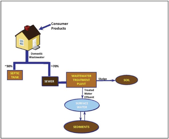
Environmental fate of surfactants from consumer products in the United States.

A. Concentration in Wastewater Effluent from Home Use

Because these chemicals are used predominantly in down-the-drain consumer and industrial products such as laundry detergents, dishwashing detergents, and personal cleansing, the first step in the pathway of these chemicals to the environment is their release from the household into the wastewater conveyance systems (Fig 3). The equation used to calculate their concentration in household wastewater, C_ww is:

(1)

where AMT is the amount of the chemical used by a person daily and W is the daily per capita water usage. The AMT is typically estimated from the tonnage of the chemical sold over a year in the country or region of interest (such as the data summarized in Section II) divided by the number of people in the population, P, and the number of days in a year (i.e., 365 days). Default values chosen for P are 3.37 × 10⁸ people (calculated from a population of 3.04 × 10⁸ people in 2008 in the United States (U.S. Census Bureau, 2008), combined with 3.33 × 10⁷ people in Canada in 2008 (Statistics Canada, 2011). The default for W was selected to be 388 L/day/person (U.S. Environmental Protection Agency [EPA], 1999 (Table 7); Kenny et al., 2009).

TABLE 7.

Recommended default values for fate assessment

Symbol	Parameter	Recommended default	Comments
P	US and Canadian Population	3.37 × 108 people	U.S. Census (2010) and Statistics Canada (2011)
W	Daily per capita wastewater	388 L/day/person	U.S. EPA (1999) and Kenny et al. (2009)
DF	Dilution factor	1 for conservative assessment, site-specific dilution factors when available
SS	Suspended solids concentration	10 mg/L	see references in Cowan et al. (1995)
SD	Sediment solids concentration	1 kg/L	see references in Cowan et al. (1995)

B. Sewer Loss

As shown in Figure 3, most domestic sewage in North America is conveyed via sewers to WWTPs. Therefore, the next step in the pathway to the surface water environment is transport in sewer conveyance systems. Although sewers were once thought to be just conveyance systems, several studies have demonstrated that these actually serve as bioreactors (Matthijs et al., 1995; Flamink et al., 2005). The approach for incorporating sewer loss into the exposure assessment is to treat sewer conveyance as a completely mixed reactor with a first-order loss rate in wastewater under conditions representative of a sewer. Typically sewers have low but not fully anoxic, dissolved oxygen levels (approximately 0.5 mg/L), subterranean temperatures, and residence times that range from a few hours to a couple of days depending on the size of the sewer system and the distance from the discharge point to the treatment plant. The average concentration in the sewer would be the influent concentration to the WWTP but if degradation has occurred, the influent concentration will be less than the concentration in the wastewater from the home estimated in Equation (1). The average concentration in the sewer, C_sew, can be calculated using the following equation:

(2)

where C_ww is the concentration in the household wastewater, k_sew is the first-order loss rate in the sewer and HRT_sew is the average hydraulic residence time for wastewater in the sewer. If information on HRT does not exist, then loss in the sewer can conservatively be assumed to be zero.

Alternatively, as is done here (see Section IV.B), the loss rate in the sewer can be estimated from the measured WWTP influent concentration compared to the estimated household wastewater concentration. Lower concentrations in the influent than those estimated from household use could also occur if the household wastewater is diluted with non-household wastewater discharged to the same sewers; therefore, to estimate the loss rate in sewers the presence of non-household discharges must be minimal. As will be discussed in Section IV.B, the measured influent concentrations in Sanderson et al. (2006b) were much lower than would be anticipated based on the amount of AE, AES, and LAS used in down-the-drain products and Equation (1) in Section III.A (Dyer, personal communication). For example, the ratio of measured to estimated influent values of AES was 0.082, meaning that nearly 98% of the AES was lost in-sewer.

C. WWTP Effluent Concentration

The main site for removal of the chemicals before entering the environment is in WWTPs (Fig 3) by sorption on sewage sludge and loss via biodegradation. The effluent concentration discharged to the surface water from WWTP, C_effluent, is calculated as:

(3)

where f_sorbed is the fraction of chemical removed via sorption onto sludge, and f_degraded is the fraction chemical removed via degradation. WWTP operational parameters (e.g., hydraulic retention time, sludge retention time) lead to variability in the overall removal of chemicals during wastewater treatment. For activated sludge plants, the effects of these operational parameters can be accounted for by wastewater simulation models (Struijs et al., 1991; Cowan et al., 1993; Lee et al., 1998; McAvoy et al., 1999). The prediction of effluent concentration, C_effluent, and sludge concentrations, C_sludge, will depend on the treatment plant operational parameters. The ASTREAT WWTP model (McAvoy et al., 1999) is useful for North American assessments.

D. Predicted Environmental Concentration in Surface Water

The bulk of WWTP effluents are released into surface waters. At the local scale, surface water concentrations at the point of the effluent discharge, C_{surface water}, can be calculated by:

(4)

where DF is the dilution factor of the volume of the effluent water in the receiving surface water. Although single default dilution factors are commonly used (U.S. Food and Drug Administration [FDA], 1998; European Commission, 2003; European Agency for the Evaluation of Medicinal Products [EMEA], 2006), in reality riverine and estuarine flow rates (and, hence, dilution) vary over several orders of magnitude depending on the flow conditions (e.g., mean or low flow), the location and season (Rapaport, 1988; Reiss et al., 2002). A default value for DF of 1, which represents no dilution of the WWTP effluent can be used to provide a conservative estimate of the surface water concentration. For this assessment, the GIS-based iSTREEM® water quality model (Wang et al., 2000, 2005), which contains WWTP infrastructure and water flow data at their discharge points across the continental United States, is used to determine individual dilution factors for each of these WWTP effluents (Section IV.B).

Once the WWTP effluent is diluted into surface waters, the processes of sedimentation and biodegradation will act to further reduce the C_surface water. The fate of the specific chemical will be dependent on the residence time of that chemical in the surface water, its sorption, and degradation properties, presence and type of suspended solids, sedimentation of solids, and presence of an active microbial community. These factors may be considered in the calculation of downstream surface water concentrations, C_downstream, by:

(5)

where f_sorb is the fraction removed during sedimentation of suspended solids; and f_biodeg is the fraction biodegraded during the travel time downstream of the effluent discharge point. Clearly, one of the chief determinants here is the duration of the travel time downstream from the point of discharge. The iSTREEM® water quality model (Wang et al., 2000, 2005) contains river flow data that is used to estimate the travel times and first-order losses due to biodegradation between points in the river system.

E. Predicted Environmental Concentration in Sediment

Any of the chemical that is attached to particles can become incorporated into sediment due to settling of these particles. A chemical's concentration in the sediment depends on the sorption constant to the suspended and sediment solids and the concentration of these solids in the water column and the sediment. The two possible calculation methods are provided below to estimate the sediment concentration.

The first is explained in detail in Cowan et al. (1995). The first step is to calculate the dry weight concentration of the chemical on the suspended particles in the water column, C_ss, using the following equation:

(6)

where K_d is the partition coefficient between suspended solids and water with units of L/kg, and SS is the suspended solids concentration with units of mg/L, and CF is the appropriate conversion factor (10⁻⁶). Next, the concentration of the chemical on the sediment solids, C_sd, is calculated using the following equation, C_sd = C_ss*SD, where SD is the sediment solids concentration in kg/L. If in addition to the concentration of the chemical on the sediment solids, the interstitial water concentration, C_iw, and/or the total sediment concentration, C_t, are needed, then these are calculated as C_iw = C_sd/K_d and C_t = C_iw + C_sd, respectively. Default values for SS and SD are 10 and 1 kg/L, respectively (Cowan et al., 1995).

Alternatively, the sediment concentration can be estimated from the surface water concentration, the organic carbon partition coefficient, K_oc, and the organic carbon content of the sediment (i.e., S_oc). This approach assumes that the sediment is in equilibrium with the overlying water which is not unreasonable for surface sediment. The equation is:

(7)

IV. EXPOSURE ESTIMATES

To conduct the prospective risk assessment of the five chemical classes, the concentrations of these chemicals in surface waters and sediments are estimated using the approach described in Section III and the specific physical, chemical, and degradation data for each surfactant in Section II. Section II of the paper presents these environmental exposure estimates. The exposure estimates will then be used with the ecotoxicity data in Section V to conduct the Prospective Risk Assessment described in Section VI.

A. Removal in Sewer Conveyance Systems

The influent adjustment factor for loss of the chemicals during transport in the sewers was determined for AE, AES, and LAS from the ratio of the average measured WWTP influent concentration determined in Sanderson et al. (2006b) to the predicted wastewater concentration from the household based on the national volume of the chemical in 2008 using Equation (1) in Section III.B (Dyer, personal communication). This ratio of measured to estimated influent values from Sanderson et al. (2006b) for AES was 0.082, meaning that nearly 98% of the AES was lost in-sewer. The in-sewer losses for AE were about 4% and for LAS were approximately 50%. The influent adjustment factors for loss of during transport in sewer conveyance systems for AS and LCOH were chosen to be the same as that for AES and AE, respectively.

B. Removal in Wastewater Treatment Systems

As described previously, to predict the concentrations in surface waters, the next step is to determine the removal of the surfactants in wastewater treatment systems. Data are available from monitoring studies at a wide range of wastewater treatment systems for these surfactants. The typical wastewater treatment systems used in North America are primary (PT), activated sludge (AST), trickling filter (TFT), rotating biological contactor (RBCT), oxidation ditch (ODT), and lagoon (LT).

1. Long-Chain Alcohols

Alkyl chain length and isotope signatures of carbon and hydrogen have been used to assess the removal of LCOHs as well as to distinguish among the sources of alcohols (i.e., natural fecal and detergent sources) in environmental media such as wastewater and receiving water sediments. Recent studies by Mudge (2012) and Mudge et al. (2008), Mudge et al. (2010), and Mudge et al. (2012) have shown that LCOHs from both fecal and detergent sources rapidly biodegrade in wastewater treatment facilities, as discussed below. In effluent, the remaining alcohols have a signature that is unlike influent, as a result of mixed-liquor in situ (bacterial) synthesis of alcohols. These studies also found that surface water and sediment alcohol signatures correspond to in situ (algae, bacteria) production or terrestrial sources (runoff of feces and/or plant-based alcohols) instead of detergent-based sources. Therefore, LCOHs measured in surface water and sediments are from natural in situ synthesis or terrestrial runoff sources not detergents.

A summary of U.S. monitoring data for total long-chain aliphatic alcohols (C_12–15) in WWTPs is presented in Table 8. Two studies reported concentrations of LCOH for AST treatment (Midwest Research Institute [MRI], 2004; Morrall et al., 2006). The average influent concentrations for LCOH ranged from 149 to 644 μg/L and average final effluent concentrations ranged from 0.22 to 0.29 μg/L. The average removal of LCOH for AST treatment in the U.S. ranged from 99.8% to 99.9% with an average removal of 99.9% from the five treatment plants monitored in these two studies. Only one study reported concentrations of LCOH for RBCT, TFT, ODT, and LT treatment (Morrall et al., 2006). For these four treatment types, the average influent concentrations ranged from 157 to 516 μg/L, the average effluent concentrations ranged from 0.06 to 3.45 μg/L, and the average removals ranged from 98.8 to 99.9%. The removal of LCOH in RBCT treatment was 99.9% (n = 1), the average for TFT treatment was 99.3 (n = 2), the average removal in ODT treatment was 99.8% (n = 2), and the average removal for LT treatment was 98.8% (n = 2). There is no information on removal of LCOH in PT treatment plants.

TABLE 8.

Monitoring data and removal values for long-chain alcohols in U.S. wastewater treatment; data for n ≥ 3 plants shown as mean ± 6SD; data for n = 2 plants shown as mean (range)

Treatment type	Number of plants	Influent (mg/L)	Final effluent (mg/L)	Final removal (%)
AST	3	0.644 ± 0.559	0.00029 ± 0.00025	99.9 ± 0.141
AST	2	0.149 (0.092–0.205)	0.00022 (0.00022–0.00022)	99.8 (99.8–99.9)2
TFT	2	0.516 (0.499–0.532)	0.0035 (0.0020–0.0049)	99.3 (99.1–99.6)2
RBCT	1	0.157	0.00006	99.92
ODT	2	0.476 (0.249–0.702)	0.00053 (0.00031–0.00074)	99.8 (99.7–99.9)2
LT	2	0.182 (0.067–0.297)	0.0015 (0.0011–0.0020)	98.8 (98.4–99.3)2

AST, activated sludge treatment; TFT, trickling filter treatment; RBCT, rotating biological contractor treatment; ODT, oxidation ditch treatment; LT, lagoon treatment.

¹MRI (2004), ²Morrall et al. (2006).

2. Alkylethoxylates

A summary of U.S. monitoring data for AEs removal in WWTPs is presented in Table 9 Because analytical methods for AE have changed, a consistent basis for comparison among the historical AE monitoring data requires that the values in the 1998 study be adjusted by a factor of 0.62 (see McAvoy et al. (2006) for details). Also, the removal values are based on measured total concentrations which include LCOH. For PT treatment, the removal was estimated based on the first stage of three activated sludge and five tricking filter plants. The removal of AE during PT treatment ranged from 18.7% to 19.3% with an average removal of AE of 18.9% (n = 8) in PT treatment.

TABLE 9.

Monitoring data and removal values for AE in U.S. wastewater treatment; data for n ≥ 3 plants shown as mean ± SD; data for n = 2 plants shown as mean (range)

Treatment type	Number of plants	Influent (mg/L)	Primary effluent (mg/L)	Final effluent (mg/L)	Primary removal (%)	Final removal (%)
AST	3	2.06 ± 60.20	1.65 ± 60.10	0.019 ± 60.022	19.3 ± 67.4	99.2 ± 60.91
AST	4	0.85 ± 60.36		0.002 ± 60.002		99.7 ± 60.32
AST	2	0.39 (0.29–0.50)		0.0007 (0.0004–0.0010)		99.8 (99.8–99.9)3
TFT	5	1.47 ± 60.63	1.20 ± 60.50	0.149 ± 60.134	18.7 ± 610.6	90.3 ± 67.21
TFT	2	1.85 (1.82–1.87)		0.0047 (0.0022–0.0073)		99.8 (99.6–99.9)3
RBCT	1	1.26		0.004		99.73
ODT	2	0.90 (0.62–1.19)		0.0022 (0.0005–0.0039)		99.8 (99.7–99.9)3
LT	2	0.84 (0.21–1.47)		0.0055 (0.0051–0.0059)		98.6 (97.5–99.6)3

AS, activated sludge treatment; TF, trickling filter treatment; RBC, rotating biological contractor treatment; OD, oxidation ditch treatment; L, lagoontreatment.

^*Values adjusted by a factor of 0.62 to account for analytical method differences between studies; see McAvoy et al. (2006) for details.

¹McAvoy et al. (1998)*; ²McAvoy et al. (2006); ³Morrall et al. (2006).

The average removal of AE for AST treatment in the United States ranged from 99.2 to 99.8% with an average removal from these three studies (McAvoy et al., 1998, 2006; Morrall et al., 2006) of 99.6% (n = 9). This U.S. removal value is similar to laboratory continuous activated sludge (CAS) studies where AE removal was >99.7% (Battersby et al., 2001; Wind et al., 2006) and to field monitoring data in Europe where AE removal was >99% (Matthijs et al., 1999).

Two studies reported concentrations of AE for TFT treatment (McAvoy et al., 1998; Morrall et al., 2006). The average TFT removal values ranged from 90.3% to 99.8% with average removal for the two studies of 93.0% (n = 7).

One study reported concentrations of AE for RBCT, ODT, and LT treatment systems (Morrall et al., 2006). For these three treatment types, the average removals ranged from 98.6% to 99.8%. The removal of AE in RBCT treatment was 99.7% (n = 1), the average for ODT treatment was 99.8% (n = 2), and the average removal for LT treatment was 98.6% (n = 2).

Thus removal of AE is greater than 90% for all wastewater treatment types except PT treatment where the removal is approximately 19%.

3. Alkylsulfates

Monitoring data for AS in WWTPs are very limited. In the United States, one study by Fendinger et al. (1992) monitored two TFT treatment plants. This monitoring study reported an average influent concentration of 578 μg/L (with a range of 401–755 μg/L), average effluent concentration of 41 μg/L (with a range of 36–46 μg/L). These values correspond to an average removal of 92% (with the range of 90–94%). Sanderson et al. (2006a) also measured >97% removal for three AST treatment plants. Matthijs et al. (1999) conducted monitoring at four oxidation ditch and one activated sludge WWTPs in Europe. An average removal for the ODT treatment plant was 99.2% with a range of 99–99.6% and for the single AST treatment plant was 99.3%. Thus, removal of AS is expected to be greater than 92% in these types of treatment plants (i.e., AST, TFT, and ODT).

4. Alkylethoxysulfates

One study (McAvoy et al., 1998) reported concentrations of alkyl ethoxylate sulfates (AES) for two AST treatment plants and four TFT treatment plants. Also, the removal values are based on total concentrations, which include AS. The average influent, effluent, and removal values for the AST treatment plants were 0.576 mg/L, 0.011 mg/L, and 98.0%, respectively (n = 2). For TFT treatment, the average influent, effluent, and removal values were 0.914 mg/L, 0.073 mg/L, and 83.5%, respectively (n = 4). Sanderson et al. (2006a) reported removals greater than 99% for three AST treatment plants.

5. Linear Alkylbenzene Sulfonates

A large number of monitoring studies have been conducted in the United States to determine the removal of LAS in various types of wastewater treatment (Table 10). Only one U.S. study reported the removal of LAS in PT treatment (Rapaport and Eckhoff, 1990) where the average removal was determined to be 27% (n = 4).

TABLE 10.

Monitoring data and removal values for LAS in U.S. wastewater treatment; data for n ≥ 3 plants shown as mean ± 6SD; data for n = 2 plants shown as mean (range)

Treatment type	Number of plants	Influent (mg/L)	Effluent (mg/L)	Removal (%)
AST	15	5.0 ± 61.9	0.04 ± 60.03	99.3 ± 60.11
AST	4	5.9 ± 62.1	0.034 ± 60.037	99.4 ± 60.12
AST	3	4.7 ± 60.8	0.004 ± 60.002	99.9 ± 60.13
TFT	12	4.2 ± 61.7	1.04 ± 60.98	77.4 ± 615.51
TFT	5	4.3 ± 661.6	0.84 ± 660.85	81.9 ± 615.42
TFT	6	4.2 ± 61.8	0.75 ± 60.57	82.3 ± 69.53
RBCT	9	4.7 ± 62.5	0.19 ± 60.38	96.2 ± 66.11
RBCT	1	2.2	0.022	99.02
ODT	6	5.7 ± 60.8	0.12 ± 60.27	98.0 ± 64.21
LT	8	4.5 ± 62.7	0.06 ± 60.01	98.5 ± 61.81
PT	4	—*	2.10 ± 60.40	27.0 ± 619.04

AS, activated sludge; TF, trickling filter; RBC, rotating biological contractor; OD, oxidation ditch; L, lagoon; P, primary.

^*Influent concentrations for the four treatment plants were not provided.

¹McAvoy et al. (1993), ²Trehy et al. (1996), ³McAvoy et al. (1998), ⁴Rapaport and Eckhoff (1990).

For AST treatment, four studies (McAvoy et al., 1993, 1998; Trehy et al., 1996; Sanderson et al., 2006b) reported average removals that ranged from 99.3% to 99.9% with an overall average removal from these studies of 99.4% (n = 25). These U.S. removal values were similar to the range of values (98.0–99.9%) reported in Europe (Cavalli et al., 1993; Waters and Feijtel, 1995; Matthijs et al., 1999) with an average removal value of 99.3% (n = 10) (Holt et al., 2003), and to laboratory CAS studies where LAS removal was greater than 99% (Cavalli et al., 1996; Leòn et al., 2006).

For TFT treatment, three studies (McAvoy et al., 1993, 1998; Trehy et al., 1996) reported average removal values that ranged from 77.4% to 82.3%. The overall average removal from these three studies was 79.7% (n = 23). These U.S. removal values are lower than those reported in Europe, which ranged from 89.1% to 99.9% (n = 24) with an average removal rate of 95.9% (Holt et al., 2003).

For RBCT treatment, two studies (McAvoy et al., 1993; Trehy et al., 1996) reported an overall average removal rate of 96.5% (n = 10). One study in the United Staes for OD treatment (McAvoy et al., 1993) reported an average removal value of 98.0% (n = 6). This average removal of LAS in OD treatment was slightly lower than the average removal rate 99.5% (n = 4) reported in Europe for OD treatment (Matthijs et al., 1999).

One U.S. study reported the removal of LAS in LT treatment (McAvoy et al., 1993). The average removal value was 98.5% (n = 8). Two studies in Europe reported removal values for LAS in LT treatment, and their average removal values ranged from 90% to 97% (Moreno et al., 1994; Marcomini et al., 2000).

C. Receiving Water Exposure Concentrations

Receiving water exposure concentrations of the chemicals were predicted using the iSTREEM® water quality model (Wang et al., 2000, 2005). iSTREEM® is a national-scale model that requires the following inputs: product chemical consumption per capita per day, removal of the chemical by wastewater treatment type, and in-stream first-order loss rates of the chemical. This information, along with effluent dilution by the receiving stream which is calculated from the WWTP flow and the receiving water flow, is used to predict receiving water concentrations under either mean or low-flow (7Q10) conditions for all U.S. rivers. The 7Q10 values represent the lowest 7-day average flow in a year that occurs during 7 consecutive days on average once every 10 years.

The input parameters used to predict receiving water exposure concentrations for each of the surfactants are provided in Table 11. The volume of the chemicals and the population numbers used to estimate the per capita use are based on 2008. As indicated in Table 11, when WWTP removal values were not available for a particular treatment plant type (e.g., ODT, RBCT, LT, and PT) for a chemical, the average of the removal values for LAS and AE in that treatment type were used since these two chemicals had complete sets of removal values across all wastewater treatment types. The in-stream degradation rates for AE, AES, and LAS were determined from river water die-away testing using the method described in Federle et al. (1997). Kikuchi (1985) and Knaggs et al. (1965) reported biodegradation half-lives for C₁₂AS ranging from 0.3 to 1 day in surface waters or a degradation rate of faster than 0.7/day using natural river waters to which the AS had been added. An in-stream loss rate of 0.7/day for LCOH, which is similar to in-stream BOD removal rates, was assumed for the loss rates of AS and LAS degradation.

TABLE 11.

Input parameters used in iSTREEM® for predicting exposure concentrations; the sources for the values are given in the text

	Chemicals
Parameters	LCOH	AE	AS	AES	LAS
North America use (metric tons)	29,000	166,070	56,000	229,330	269,000
Per capita use (g/cap/d)	0.24	1.35	0.454	1.86	2.18
Influent adjustment factors	0.86	0.86	0.082	0.082	0.5
Adjusted per capita use (g/cap/d)	0.202	1.158	0.037	0.153	1.091
WWTP process
Activated sludge	99.9	99.6	99.3	98.0	99.4
Oxidation ditch	99.8	99.8	99.2	97.3*	98.0
Rotating biological contactor	99.9	99.7	96.6*	96.6*	96.5
Lagoon	98.8	98.6	97.0*	97.0*	98.5
Trickling filter	99.3	93.0	92.0	83.5	79.7
Primary	22.6*	18.9	22.6*	22.6*	27.0
In-stream degradation
River loss (d−1)	0.7	31.2	0.7	24	0.7

^*Based on removals of LAS and AE.

The predicted exposure concentrations from iSTREEM® (presented as percent of U.S. river miles < concentration) for mean and 7Q10 (low) flow conditions for each of the chemicals are presented in Tables 12 and 13. Under low flow conditions, 90% of the river miles in the United States are expected to have concentrations of LCOH <0.0041 mg/L, AE <0.0053 mg/L, AS <0.0027 mg/L, AES <0.0053 mg/L, and LAS <0.074 mg/L under low flow conditions. Likewise, 90% of the river miles are expected to have concentrations of LCOH <0.00032 mg/L, AE <0.00089 mg/L, AS <0.00048 mg/L, AES <0.00093 mg/L, and LAS <0.014 mg/L under mean flow conditions.

TABLE 12.

Exposure concentrations predicted by iSTREEM® for LCOH, AE and AS (presented as% of U.S. river miles < concentration) for mean and low (7Q10) flow conditions

Percentile River miles (%)	LCOH (mg/L) Mean flow	LCOH (mg/L) Low flow	AE (mg/L) Mean flow	AE (mg/L) Low flow	AS (mg/L) Mean flow	AS (mg/L) Low flow
90	3.2 × 10−4	4.1 × 10−3	8.9 × 10−4	5.3 × 10−3	4.8 × 10−4	2.7 × 10−3
75	1.4 × 10−5	3.3 × 10−4	1.4 × 10−5	2.5 × 10−4	1.2 × 10−5	3.5 × 10−4
50	1.6 × 10−6	1.5 × 10−5	< 1.0 × 10−8	< 1.0 × 10−8	1.4 × 10−6	1.5 × 10−5
25	< 1.0 × 10−8	1.0 × 10−8	< 1.0 × 10−8	< 1.0 × 10−8	4.0 × 10−8	1.0 × 10−8
10	< 1.0 × 10−8	< 1.0 × 10−8	< 1.0 × 10−8	< 1.0 × 10−8	< 1.0 × 10−8	< 1.0 × 10−8

TABLE 13.

Exposure concentrations predicted by iSTREEM® for AES and LAS (presented as% of U.S. river miles < concentration) for mean and low (7Q10) flow conditions

Percentile River miles (%)	AES (mg/L) Mean flow	AES (mg/L) Low flow	LAS (mg/L) Mean flow	LAS (mg/L) Low flow
90	9.3 × 10−4	5.3 × 10−3	1.4 × 10−2	7.4 × 10−2
75	1.4 × 10−5	2.6 × 10−4	3.9 × 10−4	1.0 × 10−2
50	< 1.0 × 10−8	< 1.0 × 10−8	3.8 × 10−5	4.1 × 10−4
25	< 1.0 × 10−8	< 1.0 × 10−8	1.1 × 10−6	2.4 × 10−7
10	< 1.0 × 10−8	< 1.0 × 10−8	< 1.0 × 10−8	< 1.0 × 10−8

Due to analytical detection limits of LCOH, AE, AS, AES and LAS, the monitoring of these chemicals in receiving waters is limited to poorly operating treatment plants (e.g., TFT) that discharge into low dilution receiving waters. Because of this, predicted exposure concentrations are used when assessing ecological risk in the prospective risk assessment (Section VI).

V. ECOTOXICITY

The objective of this section is to describe how the predicted no-effect concentration (PNEC) for each of the surfactants is derived. These PNEC values are then used in conducting the prospective risk assessment (Section VI). The mechanism of toxicity for surfactants is accepted to be nonpolar narcosis in which the surfactant's presence in the cell membrane is believed to interfere with membrane-dependent life processes such as energy metabolism and transport of nutrients and oxygen across the membrane. For example, the toxicity of several anionic and nonionic surfactants has been observed to be highly correlated with properties like standard free energies and interfacial activity (Rosen et al., 1999, 2001), longer hydrocarbon chains, and higher log K_ow, which led to more efficient penetration of the cell membrane, supporting the hypothesis that the toxicity of surfactants is determined by adsorption on biological membranes and cell membrane penetration. Both the nature of the hydrophobe (the alkyl chain) and the nature of the hydrophilic head group contribute to defining the magnitude of these properties for a specific surfactant homologue. The hydrophobe determines the ease with which the surfactant will insert itself into the membrane bilayer and the amount of disturbance due to hydrophobic interactions caused once it is in the membrane. This explains the observed pattern, typical for the ecotoxicity of surfactants in general, of increasing toxicity with increasing alkyl chain length—until a point is reached where water solubility becomes the limiting factor. For several of the very long-chain length surfactants, solubility is greatly reduced and thus the toxicity decreases, especially for hydrocarbon chain lengths of 15 and above. Bernhard and Dyer (2005), using cellular levels of surfactants (including LAS and AE), verified a narcotic mechanism of action where the lethal concentration for fish hepatic cells was approximate to fish tissue residues associated with narcosis.

The PNEC for the aquatic environment can be determined in several ways based on the quantity of and species and taxa range covered by the available acute, chronic, and mesocosm toxicity data and whether any reliable QSARs have been developed from these data. For small data sets, the PNEC is estimated using the most toxic standardized (e.g., LC/EC50, no-observed-effect-concentration (NOEC)) end point and applying an assessment factor (AF) that is consistent with the amount and type of data available (Cowan et al., 1995). These surfactants all have large sets of acute and chronic toxicity data, and in many cases mesocosm data; therefore, this simple method is not used. For surfactants with larger data sets of chronic toxicity data, the PNEC can be estimated using several approaches. To apply these approaches, the aquatic toxicity data are first normalized to an environmentally relevant homologue or distribution based on monitoring studies, if available, (e.g., individual chronic toxicity data for LAS is normalized to C_11.6). If there is a large set of chronic toxicity data across a wide range of species and taxa, then the PNEC can be determined using a species sensitivity distribution (SSD) based on these normalized data using the methods of van de Plaasche et al. (1999). SSDs can be used to calculate the concentration at which a specified proportion of species are expected to suffer toxic effects. This concentration is estimated by maximum likelihood assuming a log-logistic (or other statistically suitable) distribution of these data values, i.e., fitting a logistic distribution to the log-transformed data values with confidence intervals on this distribution computed by the methods of Aldenberg and Slob (1993). The interval on the HC₅ (5th percentile of the SSD) is intended to ensure that there is a high probability (95%) that the true HC₅ is within the limits of the interval, based upon the model fitted to the data. The PNEC is estimated by this HC₅ with no additional application factor if sufficient data of high quality are available (European Chemicals Agency, 2008). This approach was used for AE, AES, and LAS. Another approach when chronic toxicity data are available but limited in the species and taxa coverage, as illustrated for LCOH and AS, is to use one or more chronic toxicity QSAR to estimate a toxicity value for the environmentally relevant homologue or distribution. Addition of measured concentration/measured or predicted effect or no effect concentrations (i.e., toxic units) can also be used for any surfactant chain length distribution since all chain lengths operate with the same mode of action. This toxic unit approach for AS and AE is described in more detail in Belanger et al. (2006) and HERA (2009b).

As compared to single-species tests, meso- or microcosm studies involving more than one species are recognized to be a better approximation of environmental reality and therefore, have a higher predictive value. Therefore, in estimating the PNEC, a smaller application factor is applied to these results if the mesocosm is suitably biologically diverse, contains sensitive flora and fauna, and the exposure is of a chronic time frame (Belanger, 1997). Typically, this AF is between one and five (Solomon et al., 2008). Thus, when there are mesocosm studies, these are of greater weight than acute or chronic ecotoxicity data when a weight-of-evidence (WoE) approach is used to estimate the PNEC for a specific homologue. These studies are also used in combination with a QSAR based on these data to extrapolate these mesocosm data to an environmental relevant homologue or distribution. Because the surfactants discussed in this paper are generally all HPV chemicals, the detergent industry devoted significant resources to develop mesocosm studies on them. Stream mesocosm studies are therefore available for AE, AES, AS, and LAS and will be discussed below. Due to the wealth of data, an AF of 1 was used for determining the PNEC for each surfactant.

A. Long-Chain Alcohols

An extensive review and summary of the LCOHs acute and chronic toxicity data with tabular summaries can be found in OECD (2006), Fisk et al. (2009), and Schäfers et al. (2009). The objective of this section is to summarize the toxicity understanding from these available data, and how these data are then used to derive the environmental relevant aquatic PNEC. The reader is recommended to refer those documents for specific details of the toxicity data studies.

1. Aquatic and Sediment Toxicity

Sufficient measured data exist to quantify the acute and chronic aquatic toxicity of essentially pure alcohols and mixtures of these alcohols to fish, invertebrates, and algae (OECD, 2006). Because alcohols act by nonpolar narcosis (Lipnick et al., 1985), read-across is scientifically justified for filling any gaps in the data. Furthermore, as discussed in Fisk et al. (2009), the toxicity of mixtures of fully dissolved alcohols can be estimated based on simple addition of the contribution of each component of the alcohol mixture. The acute and chronic toxicity data for LCOH which are discussed below are summarized in Table 14.

TABLE 14.

Range of acute and chronic toxicity of LCOH to algae, invertebrates, and fish

	Chain length	End point	Range (mg/L)
Acute toxicity
Algae	C6–C16	72 hr EC50	80 (C6)–0.97(C12)
Aquatic invertebrates	C6–C14	24–96 hr EC50	200 (24 hr C6)–0.77 (48 hr C12)
Fish	C6–C22	96 hr LC50	97 (C6)–>0.33 (C13)
Chronic toxicity
Algae	C6, C12	NOEC 72 hr	11 (C6), 0.40 (C12)
Aquatic invertebrates	C8–C15	EC10 survival	1.0 (C8)–0.033 (C12)
		EC10 reproduction	1.0 (C8)–0.0063 (C14)
Fish	C6	NOEC 7d	0.75–3

The best quality acute toxicity data on single carbon chain linear alcohols from C₆ to C₂₂ (OECD, 2006; Fisk et al., 2009) for fish show that the toxicity of the single carbon number chain length alcohols increases from an LC₅₀ of 97 mg/L for C₆ to 1.0 mg/L for C₁₂. At higher carbon numbers up to C₂₂, the measured acute toxicity shows an absence of acute toxicity as evidenced by reported LC₅₀ values that are greater than the highest test concentration. This is explained by the low water solubility of these LCOHs, which limits their bioavailability, such that an acutely toxic concentration is not achieved (Fisk et al., 2009). The best quality invertebrate acute toxicity data for single carbon chain length linear alcohols from C₆ to C₁₄ (OECD, 2006) show the toxicity of the alcohols increases from an EC₅₀ of 200 mg/L for C₆ to 0.77 mg/L for C₁₂. Effects have also been observed in tests with C₁₃ and C₁₄ alcohols but at concentrations that exceeded the solubility of the alcohols; therefore, the observed toxicity may be due to physical effects (rather than true toxicity) for these two alcohols (OECD, 2006). The best quality algal toxicity data for single carbon chain lengths from C₆ to C₁₆ (OECD, 2006) show the toxicity of the alcohols to increase from an E_rC₅₀ of 80 mg/L for C₆ to 0.62 mg/L for C₁₂. The C₁₄ and C₁₆ alcohols were not toxic to algae. These results suggest that for alcohols in the range of C₁₂–C₁₄, there are no acute toxicity effects on fish, invertebrates, and algae driven by the low solubility of these alcohols, although there may be physical effects and that the three types of organisms are about equally sensitive acutely to alcohols of the same chain length (Table 14).

The acute toxicity data for fish, invertebrates, and algae to multicomponent substances of different carbon chain length alcohols as would be found in commercial products (OECD, 2006) have also been determined. These multicomponent substances containing alcohols with carbon numbers in the ranges of C₆–C₁₂, where all the components would be completely dissolved, are acutely toxic at concentrations as expected from the contribution of the individual linear alcohols to the mixture. By contrast for multicomponent substances which contain one or more alcohols with chain lengths greater that C₁₂–C₁₄, where not all components were fully dissolved, toxicity not only appears to be the result of toxic effects from the soluble portion of the alcohols but also includes toxic effects as a result of physical fouling of the test organism by the longer-chained alcohols.

This extensive acute toxicity database for these pure linear alcohols (OECD, 2006) was used to derive specific QSARs for fish and Daphnia magna as a function of log K_ow (Fisk et al., 2009) Insufficient data are available to develop a QSAR for algae.

The acute toxicity QSAR for fish is:

96-h log LC₅₀ in mmol/L = −0.691log K_ow + 1.29

And for Daphnia is:

48-h logEC₅₀ in mmol/L = −0.83 log K_ow + 1.92

Chronic aquatic toxicity data for fish and algae (OECD, 2006) are limited to one or two studies (Table 14). Invertebrates, represented by D. magna, have a robust database of 21-day chronic toxicity data across a range of chain lengths from C₈ to C₁₅. These data were used by Schäfers et al. (2009) to develop a set of QSARs for chronic toxicity represented by mortality/survival and reproductive effects based on the initial mean concentration or total mean concentration of the alcohol. These QSARs are

Mortality:

• log EC₁₀ (μmol) = −0.36 log K_ow + 2.13 (initial mean concentration)

• log EC₁₀ (μmol) = −0.63 log K_ow + 2.92 (total mean concentration)

Reproduction:

• log EC₁₀ (μmol) = −0.49 log K_ow + 2.54 (initial mean concentration)

• log EC₁₀ (μmol) = −0.88 log K_ow + 3.80 (total mean concentration)

These QSARs show that the chronic response of D. magna is consistent with a nonpolar narcotic mode of action as discussed in Schäfers et al. (2009).

There are no data on the acute or chronic toxicity of alcohols to sediment dwelling organisms.

2. Predicted No-Effect Concentration

As described in OECD (2006), available data suggest that the three taxonomic groups—fish, invertebrates, and algae—are of comparable susceptibility to the individual long-chain aliphatic alcohols, consistent with narcosis structure activity. Therefore, the database for chronic aquatic effects of single carbon number alcohols from D. magna reproduction tests was used to estimate the aquatic PNEC for each of the individual chain lengths. The PNEC was estimated by dividing the NOEC value for the D. magna, either measured or estimated using the QSAR derived for reproductive effects, by an AF of 10. Justification for use of the AF of 10 can be found in Belanger et al. (2009). Furthermore, it is assumed that for alcohols with chain lengths >C₁₅, there will be no chronic effects and thus no appropriate PNEC. The PNEC values are given in Table 15.

TABLE 15.

Measured or predicted NOEC as well as PNEC for ecosystem protection for LCOH chain lengths ranging from 6 to 14 carbon units

Chain length	Chemical name	Measured or predicted NOEC (mg/L)	PNEC (mg/L)
C6	1-Hexanol	6.8	0.680
C8	1-Octanol	1.0	0.100
C10	1-Decanol	0.11	0.011
C11	1-Undecanol	0.17	0.017
C12	1-Dodecanol	0.014	0.0014
C13	1-Tridecanol	0.046	0.0046
C14	1-Tetradeconal	0.0016	0.00016

However, in the environment, the alcohols will not appear as individual chain lengths but rather as mixtures of chain lengths as evidenced by monitoring studies of WWTP effluents in North America (Dyer et al., 2006a, 2006b; Eadsforth et al., 2006; Morrall et al., 2006). The most prominent chain length found in those sewage treatment plant effluents across a wide range of treatment types, including lagoons, oxidation ditches, trickling filter, activated sludge and rotating biological contactor, was C₁₂–C₁₈. As described previously, because of the low solubility of LCOH with chain lengths greater than C₁₅, no toxic effects will be exerted by these longer chain lengths, and these are thus eliminated from this analysis (Belanger et al., 2009). The average chain length based on the range of C₁₂–C₁₅ in the effluent is C_13.3 (based on data in table 3 of Belanger et al., 2009). The average chain length based on the range of C₁₂–C₁₅ was C₁₃ after correction was made to the effluent concentrations based on bioavailability corrections for each of the monitored sites (based on data in table 4 of Belanger et al., 2009). The resulting PNEC for C₁₃LCOH would then be 0.0046 mg/L (Table 15).

Because there are no data on the acute or chronic toxicity of alcohols to sediment dwelling organisms, no PNEC can be estimated for LCOH in sediment.

3. Bioconcentration Factor

No reliable guideline-standard measured bioconcentration factors (BCFs) are available for the LCOHs in part because of their rapid degradation (OECD, 2006; Fisk et al., 2009). BCF values can be estimated using available QSARs such as Veith et al. (1979), Connell and Hawker (1988), and the BCFBAF module in EPI Suite^TM v4.10 (http://www.epa.gov/opptintr/exposure/pubs/episuitedl.htm). As discussed in Fisk et al. (2009), Veith et al. (1979), and Connell and Hawker (1988), QSARs tend to result in overly conservative estimates of the BCF because these do not include the impact of biotransformation of alcohols. Biotransformation would be expected since alcohols serve as an energy source (food) through metabolism for a wide range of biota from bacteria to mammals (Mudge et al., 2008; Veenstra et al., 2009). The BCFBAF module estimates a biotransformation half-life in a 10 g fish of from 0.146 days for 1-hexanol to 21 days for 1-docosonol with estimated BCF of 6.6 and 13.7, respectively. Branched structures are predicted to have slightly lower BCF values than the corresponding linear alcohols consistent with their lower log K_ow.

B. Alkylethoxylates

An extensive review and summary of the AE acute and chronic toxicity data with tabular summaries can be found in Belanger et al. (2006), HERA (2009b), and Madsen et al. (2001). The objective of this section is to summarize the toxicity understanding from the available data, and how these data are used to derive the environmentally relevant PNEC for AE. The reader is recommended to refer those documents for details of the data and any particular studies.

1. Aquatic and Sediment Toxicity

Acute aquatic toxicity studies to AE homologs and commercial mixtures have been conducted for a wide range of species, life forms, feeding strategies, and trophic levels, including green and blue-green algae, diatoms, saltwater shrimp, freshwater isopods, freshwater flatworms, freshwater midge larva, Daphnia, and a wide range of both freshwater and saltwater fish species (Madsen et al., 2001; HERA, 2009b). These data (Table 16) illustrate that algae appear somewhat more sensitive to AE than either invertebrates or fish. The acute fish, invertebrate, and algal acute eco-toxicity test results also indicate that the branched and essentially linear AE are not more toxic than the linear AE of the same hydrocarbon chain length and EO number. The acute toxicity data also show that toxicity decreases with increasing EO chain length and increases with increasing hydrocarbon chain length, so long as the AE remains soluble in water. For example a C_14–15EO₇ is more toxic than a C_9–11EO₆, essentially demonstrating carbon chain length effects (Wong et al., 1997).

TABLE 16.

Ranges of acute toxicity for AE to algae, invertebrates and fish

	AE	End point	Range (mg/L)
Algae	Linear AE	72 hr EC50	0.05 (C15 EO7–8) to 50 (C12–14EO9)
	Branched AE	72 hr EC50	0.05 (C15 EO7–8 25% branching) to 50 (Iso-C10 EO7–8 highly branched)
Aquatic invertebrates	Linear AE	LC50	0.1 (C13EO1) to > 100 (C16–18 EO4–7)
	Branched AE	LC50	0.5 (C13 EO7–8 10% branching and C15 EO7–8 25% branching) to 50 (Iso-C10 EO7–8 with 3 internal CH3-groups, highly branched)
Fish	Linear AE	LC50	0.4 (C16–18 EO14) to > 100 (C16–18EO204)
	Branched AE	LC50	0.25 (oxy-C9–15 EO2) to 40 (oxy-C9–15 EO>10)

Sources: Madsen et al. (2001); HERA (2009b).

Chronic aquatic toxicity (Table 17) has also been determined for 17 different aquatic species, ranging from algae, Daphnia, mollusks, rotifers, and to several fish species, for AEs representing a range in hydrocarbon chainlength distribution and the EO chainlength distribution (HERA, 2009b). These studies were most recently summarized by HERA (2009b), Belanger et al. (2006), Belanger and Dorn (2004), and in the Dutch Risk Assessment of Surfactants, summarized in van de Plaasche et al. (1999). These studies demonstrate that the rainbow trout, a mollusk (clam), and rotifers are amongst the most sensitive taxa, although differences in sensitivity across trophic levels were not significantly different (Belanger et al., 2006, Table 16). As was seen with acute toxicity, chronic toxicity increases with increasing hydrocarbon chain length and decreases with increasing EO chainlength.

TABLE 17.

Ranges of chronic toxicity of AE to algae, invertebrates, and fish

	Species and lifestage	End point	Range (mg/L)
Algae	Desmodesmus (Scenedesmus)subspicatus and Pseudokirchneriella subcapitata (Selenastrum caprcicornutum) (Growth rate)	EC10	0.03 (C12EO2) to 9.791 (C8–10 EO5)
Aquatic invertebrates	Daphnia (reproduction) and Hyallela (larvae survival), respectively.	LC10	0.082 (C12–15 EO6) to 3.882 (C9–11EO6)
Fish	Rainbow trout egg to alevin weight gain and Bluegill juvenile survival, respectively	LC10	0.079 (C12–15EO9) to 8.983 (C9–11EO6)

Source: HERA (2009b).

The relationship between hydrophobicity and toxicity demonstrated by both the complete acute and chronic toxicity data sets were used as the basis for developing AE chronic QSARs for algae, Daphnia, and fish based on selected studies of specific AE homologues and their K_ow. The algal QSAR was based on the EC₂₀ values determined for Desmodesmus subspicatus for biomass/yield from a high-quality study of the toxicity of six AE homologues ranged from 10 to 16 carbons in the hydrocarbon chain and from 2 to 8 EO groups (Wind and Belanger, 2006). The resulting QSAR is

72-h EC₂₀ in mM = 10^{−0.378*log K_ow−4.072}

The chronic D. magna QSAR was developed from seven data sets measuring the most sensitive end point, survival, for six distinct AE homologue mixtures (see Boeije et al. (2006) for details on the studies selected). The AE homologues provided a good representation of the hydrocarbon range from C₉ to C₁₅ and good coverage of the EO range from 0 to 15. The resulting QSAR is

21-day EC₂₀ in μ mol/L = 10^{−0.532*log K_ow+2.975}

The chronic fish QSAR was developed by Boeije et al. (2006) using a high-quality data set obtained by Lizotte et al. (1999). This data consisted of an early life stage study for fathead minnow (Pimephalespromelas) exposed to three AE surfactant mixtures (C_9–11EO6, C_12–13EO_6.5, and C_14–15EO₇). Due to the limited number of data points, Boeije et al. (2006) consider the QSAR to be of low reliability. The resulting QSAR is

28-day EC₂₀ in μ mol/L = 10^{−0.307* log K_ow+2.08}

As can be seen by comparing the three QSARs, their slopes (range −0.3 to −0.5) and intercepts (range −3 to −4) are very similar. Thus, Wind and Belanger (2006) concluded that no one trophic group appears to be uniquely sensitive or insensitive to AEs, based upon the chronic data. Belanger et al. (2006) used this observation as the basis for determining SSD for all the AE homologues and from this the HC5 using the methods of Aldenberg and Jaworska (2000) and Van Vlaardingen et al. (2003).

AEs have an unparalleled set of mesocosm studies (Table 18). These are summarized in Belanger et al. (2000). These studies came from a strategy to test the range of commercial mixtures from a relatively low alkyl carbon range (C₉–C₁₁) to relatively high (C_14–15) and short (6) to moderate (9) ethoxylation. Studies were detailed ecological investigations including microbial and invertebrate communities and caged fish of 1–2 months duration of exposure to the test materials. The NOECS of these AE mesocosm studies were found to be very similar to the HC5s from SSDs using chronic toxicity data (Mitchell et al., 1993; Tattersfield et al., 1995; Dorn et al., 1996a, 1996b, 1997a, 1997b; Harrleson et al., 1997; Lizotte et al., 1999; Belanger et al., 2000; Wong et al., 2004; Belanger et al., 2006). Boeije et al. (2006) used these underlying data to develop an average-structure QSAR at the ecosystem level:

TABLE 18.

Summary of model ecosystem studies conducted on AE

AE tested	Location of study	NOEC (μg/L)	LOEC (μg/L)	Principal effects
45-7	University of Mississippi	80	160	Simulium abundance
23-6.5	University of Mississippi	—	320	Invertebrate abundance reduced; loss of Simulium
91-6	University of Mississippi	730	2040	Fathead minnow survival and reproduction
25-9	Shell Sittingbourne Research Center, UK	70	160	Simulium and Gammarus abundance reduced
25-6	P&G, Cincinnati, OH	13	37	Several taxa and total invertebrate abundance and richness reduced

Source: Table 5 in Belanger et al. (2000).

mesocosm NOEC in μ g/L = 10^{−0.74×K_ow−2:78}

Both the acute and chronic aquatic toxicity data sets for sediment dwelling taxa, such as Chironomus tentans and Corbicula fluminea, and others which live near or in the top sediment surface such as Hyallela azteca, Dugesia gonocephala, Chlorella vulgaris, and Navicula pelliculosa. Aquatic macrophytes have also been assessed (Lemna minor). These aquatic test data (Table 19) are reported as the concentration in the water above the sediment. The lowest EC₁₀ value for C_12–15EO₆ of 0.062 mg/L is for C. fluminea based on length growth.

TABLE 19.

AE toxicity for aquatic species that live in sediment or top surface of the sediment

Species name	Life stage	Compound	Most sensitive end point	Effect conc (EC10) (mg/L)
Chlorella vulgaris	Vegetative	C12–15EO3	Growth rate	2.179
Chironomus tentans	Larvae	C9–11EO6	Survival	3.635
Hyallela azteca	Larval	C9–11EO6	Survival	3.882
Dugesia gonocephala	Immature	C14EO10	Survival	0.840
Navicula pelliculosa	Vegetative	C14–15 EO7	Cell density	0.140
C. fluminea	Juvenile	C12–15EO6	Length gain	0.062

Source: Table 1 in Belanger et al. (2006).

2. Predicted No-Effect Concentration

Given the plethora of data, the PNEC for AE in the aquatic environment can be determined in several ways based on the acute and chronic toxicity data used, QSARs, and mesocosms. These alternative PNEC derivation methods are explained in detail in Belanger et al. (2006) and HERA (2009b) and include (1) using the chronic D. magna QSAR and applying an AF, (2) using the chronic probabilistic QSAR approach, and (3) using a mesocosm-based QSAR. These approaches and resulting PNEC are based primarily on chronic AE effects data and QSARs that have been determined for linear AEs. The use of this linear AE data is considered appropriate because the acute toxicity data show that the toxicity is essentially the same for the essentially linear and branched AEs.

Using the first approach, namely the chronic D. magna QSAR (Boeije et al., 2006) and an AF of 10, which is probably conservative, was applied to the QSAR results for each AE homologue to determine the PNEC (HERA, 2009b). Using this approach for the range of potential AEs in the environment, the PNEC for C₈EO₃ is 0.4 mg/L and for C₁₈EO₁₂ is 0.009 mg/L.

The second approach, namely the chronic probabilistic QSAR from Belanger et al. (2006), is essentially an SSD approach where the chronic QSARs for D. subspicatus, D. magna, and P. promelas are applied to algae, invertebrates, and fish to estimate the PNEC for a particular AE homologue. The reader is referred to Belanger et al. (2006) for details on the approach. No additional AF is required to be applied to the resulting chronic toxicity SSD because of the high quality of the data (approximately 60 chronic studies) and the range of species (17 different taxa) represented by the QSARs. The full set of PNEC values calculated using this approach is given in table 4 of Belanger et al. (2006) and presented in Table 20. The corresponding PNEC values for C_8–9E₃ is 0.271 mg/L and that of C₁₈E₁₂ is 0.0179 mg/L, using this approach are very similar to those estimated using the first approach based on the Daphnia QSAR.

TABLE 20.

Predicted HC5 values (mg/L) for pure AE homologs using chronic probabilistic QSAR

Ethoxylate chain length	Alkyl chain length
	C9	C10	C11	C12	C13	C14	C15	C16	C18
	3	0.2706	0.1845	0.1232	0.0801	0.0505	0.0307	0.0181	0.0103	0.0031
4	0.3394	0.2305	0.1536	0.0998	0.0629	0.0384	0.0226	0.0129	0.0039
5	0.4174	0.2828	0.1882	0.1223	0.0773	0.0472	0.0279	0.0160	0.0048
6	0.5056	0.3421	0.2276	0.1481	0.0937	0.0575	0.0341	0.0196	0.0059
7	0.6050	0.4091	0.2723	0.1774	0.1126	0.0693	0.0412	0.0237	0.0072
8	0.7169	0.4846	0.3227	0.2106	0.1341	0.0828	0.0495	0.0286	0.0088
9	0.8425	0.5695	0.3795	0.2482	0.1585	0.0983	0.0590	0.0342	0.0106
10	0.9831	0.6647	0.4434	0.2906	0.1861	0.1159	0.0698	0.0407	0.0127
11	0.1404	0.7712	0.5151	0.3383	0.2173	0.1359	0.0823	0.0482	0.0151
12	0.3159	0.8903	0.5953	0.3918	0.2525	0.1585	0.0965	0.0568	0.0179

Source: Table 4 in Belanger et al. (2006).

The final approach is to use the data from the mesocosm studies (Table 19) on various AEs which were conducted in the mid-1990s to derive a PNEC. The AE mixtures represented in these mesocosm studies cover the full range of commercially relevant uses in detergents. Belanger et al. (2000) provide a review of the mesocosm studies and, as mentioned previously, Boeije et al. (2006) developed a nonlinear QSAR based on a toxic unit approach for these studies. Toxicity predictions based on both the previous approaches and this mesocosm approach provided very similar results. The fact that mesocosm and the chronic toxicity QSAR outcomes are so similar supports the use of no additional application factor to the results in Table 19. Ultimately, the SSD approach, approach two, is considerably more flexible and spans a greater range of AE mixtures and is, therefore, used to develop the PNEC for the environmentally relevant form of AE.

The average AE in effluents in the United States is C_14.7EO_9.1 and in Canada is C_13.6EO_8.4 (Belanger et al., 2006, table 2). Based on this average distribution of AE structure in effluent and the HC₅ values in Belanger et al. (2006) and Table 19 which are based on the second approach, the HC₅ which will be used to represent the aquatic PNEC for the North America would be the range of 0.0983 mg/L (U.S. average structure) to 0.1341 mg/L (Canadian average structure).

The limited toxicity data for sediment dwelling or associated organisms suggest that this same PNEC could be used to represent sediment toxicity when expressed as the interstitial water concentration because the EC₁₀ value for the most sensitive chronic end point for a sediment dwelling taxa of 0.062 mg/L is within the range of EC₅ values for that range of alkyl chain lengths (i.e., 0.1481 (C₁₂) to 0.0341 (C₁₅) mg/L) with an ethoxylate chain length of 6 units (Table 19).

3. Bioconcentration Factor

Bioaccumulation of AE in aquatic organisms had been determined only for fish (Madsen et al., 2001). Furthermore, the majority of the limited data were based on studies with ¹⁴C-labeled compounds that do not allow the distinction between the parent compound and metabolites, or material incorporated into the cells during growth. Because AEs are metabolized in aquatic organisms (Madsen et al., 2001; Dyer et al., 2008), the BCF for the parent compound may well be overestimated in experiments in which ¹⁴C-labeled model surfactants are used. Tolls (1998) and Tolls et al. (2000a) combined ¹⁴C-techniques and chemical analysis to determine the amount of AE actually present as the parent molecule in the fish. This showed that the parent AE (e.g., C₁₃EO₈) was rapidly eliminated by transformation into metabolites, which were eliminated at a slower rate. The BCF factors which Tolls obtained using this combined technique for several AE homologues in fathead minnow range from <5 for C₁₄EO₁₄ to 387.5 for C₁₆EO₈ (HERA, 2009b). The time to steady state and the BCF for AE increase with decreasing length of the ethoxylate chain (e.g., t₉₅ for C₁₃EO₈ = 2.4 hr and BCF = 30–55, and t₉₅ for C₁₃EO₄ = 17.1 hr and BCF = 233) (Madsen et al., 2001). Environment Canada and Health Canada (2006) found that the 16 measured BCF values for 15 AE homologues showed a lack of a linear relationship between alkyl or ethoxylate chain length and BCF. They concluded that the AE metabolism rates prevent any significant accumulation.

C. Alkylsulfates

An extensive review and summary of the AS acute and chronic toxicity data with tabular summaries can be found in HERA (2002), OECD (2007), Könnecker et al. (2011), and BUA (1996). The objective of this section is to summarize the toxicity understanding from the available data and how these data are used to derive the environmentally relevant PNEC for AE. The reader is recommended to go to those documents for specific details of the toxicity studies.

1. Aquatic and Sediment Toxicity

Extensive acute and chronic toxicity data to fish, both freshwater and marine species, invertebrates, and algae for AS ranging from chainlengths of C₈–C₁₈ both as single chainlengths and in mixtures of chain lengths, are presented in HERA (2002) and OECD (2007). The lowest acute and chronic toxicity values from this extensive database are summarized in Tables 21 and 22, respectively. While data exist for chain lengths ranging from C₈ to C₁₈, the homologue C₁₂ has the largest ecotoxicological database of the group. Due to AS's susceptibility to biodegradation and propensity to form calcium salts especially at the longer chainlengths, greatest confidence is given to the results from toxicity tests that utilize flow-through or static/renewal exposure methods with measured concentrations.

TABLE 21.

Summary of lowest acute aquatic toxicity data for AS

Chain length	Species	Toxicity end point	Value (mg/L)
C8
Fish	Leuciscus idus	48 hr LC50	1721
Aquatic invertebrates	D. magna	24 hr EC50	43502
C9
Aquatic invertebrates	D. magna	24 hr EC50	23002
C10
Fish	Cyprinus carpio prelarva	48 hr LC50	133
Aquatic invertebrates	D. magna	24 hr EC50	4704
C12
Fish	Cyprinus carpio prelarva	48 hr LC50	133
Aquatic invertebrates	C. dubia	48 hr EC50	5.555
Algae	Pseudokirchneriella subcapitata	96 hr EC50	1176
C13
Fish	Leuciscus idus	48 hr LC50	2.17
Aquatic invertebrates	D. magna	24 hr EC50	422
C14
Fish	Oryzias latipes	48 hr LC50	2.58
Aquatic invertebrates	C. dubia	48 hr EC50	1.585
C15
Fish	Leuciscus idus	48 hr LC50	159
Aquatic invertebrates	C. dubia	48 hr EC50	0.595
C16
Fish	Oryzias latipes	48 hr LC50	0.53
Aquatic invertebrates	C. dubia	48 hr EC50	0.155
C18
Fish	Leuciscus idus	48 hr LC50	>27010
Aquatic invertebrates	C. dubia	48 hr EC50	>0.695
C10–16
Algae	Pseudokirchneriella subcapitata	72 hr EC50	6011
C12–14
Algae	D. subspicatus	72 hr EC50	2712
C12–18
Algae	D. subspicatus	96 hr EC50	3813
C14–15
Algae	Pseudokirchneriella subcapitata	72 hr EC50	4.614
C16–18
Algae	D. subspicatus	72 hr EC50	3415

¹Cognis (2001a) in OECD (2007), ²Lundahl and Cabridenc (1978), ³Kikuchi et al. (1976),⁴Sánchez Leal et al. (1991),⁵Dyer et al. (1997), ⁶Nyholm and Damgaard (1990), ⁷Cognis (2006a) in OECD (2007), ⁸Kikuchi and Wakabayashi (1984), ⁹Cognis (2006c) in OECD (2007), ¹⁰Cognis (2001f) in OECD (2007), ¹¹Yamane et al. (1984), ¹²Verge and Moreno (1996), ¹³Henkel KGaA (1992g) in OECD (2007), ¹⁴Procter & Gamble (1986) in OECD (2007),¹⁵Cognis (2001ee) in OECD (2007).

TABLE 22.

Summary of lowest chronic aquatic toxicity data for AS

Chain length	Species	Test method	NOEC (mg/L)
C12
Fish	P. promelas Larva	42 day, flow through	>1.361
Bivalves	Corbincula fluminea	42 day, flow through	0.4181
Mollusks	Goniobasis	42 day, flow through	>1.361
Insects	Lymnephilus Larva	42 day, flow through	>0.4181
Aquatic invertebrates	Brachionus calyciflorus	2 days life cycle test, static	EC20 = 0.772
Algae	D. subspicatus	72 hr, static	303
Algae	Pseudokirchneriella subcapitata	4 days, growth inhibition	EC10 = 124
C14
Aquatic invertebrates	C. dubia	7 days, flow through	LOEC5<0.062
C15
Aquatic invertebrates	C. dubia	7 days, flow through	0.2305
C16
Aquatic invertebrates	C. dubia	7 days, flow through	0.2045
C18
Aquatic invertebrates	C. dubia	7 days, flow through	0.6025
C12–18
Algae	D. subspicatus	OECD 201	0.96
C14–15
Fish	P. promelas	34-day early life stage test, flow- through	0.117
Aquatic invertebrates	C. dubia	7 days, flow through	0.815
C16–18
Fish	Danio rerio	OECD 204	1.78
Aquatic invertebrates	D. magna	OECD 202	16.58
Algae	D. subspicatus		349

¹Belanger et al. (1995b), ²Versteeg et al. (1997), ³Henkel KGaA (1994) in OECD (2007), ⁴Nyholm and Damgaard (1990), ⁵Dyer et al. (1997), ⁶Henkel KgaA (1992g) in OECD (2007), ⁷Procter & Gamble (1987) in OECD (2007), ⁸Steber et al. (1988), ⁹Cognis (2001ee) in OECD (2007).

The acute toxicity database (Table 21) for fish is quite extensive with reliable studies available for 13 different species covering a variety of both freshwater and marine species (OECD, 2007). According to Könnecker et al. (2011), the acute toxicity to freshwater and marine fish for chain lengths of C₈–C₁₂ (13–172 mg/L) is considered to be low to moderate over a range of toxicity end points (e.g., 48-h LC₅₀, 96-h EC₅₀). The acute toxicity increases with increasing chain length with the most toxic chainlengths, C₁₃–C₁₅ having 48-h LC₅₀ values ranging approximately from 2 to 15 mg/L. For those AS chain lengths up to C₁₆, toxicity values appear to be independent of the fish species tested, the counterions present or the test conditions. In fact, the range in toxicity is rather homogenous for a given chain length in this range despite toxicity tests done with highly varied exposure methods (i.e., static, semistatic, and flow-through), and whether they used nominal or measured concentrations (Könnecker et al., 2011). There also appears to be no influence of the counterion (e.g., Na, K, Mg, NH₄, monoethanolamine, TEA salts) on toxicity. Studies examining the influence of water hardness on the toxicity of AS do not reveal a consistent relationship (Könnecker et al., 2011). The toxicity reported for AS of chain lengths of C₁₆ and higher are inconsistent, probably due to variability in bioavailability as a result of reduced water solubility.

A broad database of reliable studies for acute invertebrate toxicity is available (Table 21), covering a range of freshwater, marine, and estuary organisms (OECD, 2007; Könnecker et al., 2011). Toxicity increased with increasing alkyl chain length for the freshwater species of D. magna (Lundahl and Cabridenc, 1978; Sánchez et al., 1991) and Ceriodaphnia dubia (Dyer et al., 1997). The Dyer et al. study, which utilized a flow-through design with analytical verification, observed a linear relationship between chain length and toxicity from C₁₂ (48-h EC₅₀ = 5.55 mg/L) to C₁₆ (48-h EC₅₀ = 0.15 mg/L). Furthermore, the Dyer et al. study observed no mortality for C₁₈AS, due to solubility limitations. In summary, for invertebrates, AS acute toxicity increases with increasing length of the hydrocarbon chain up to C₁₆ and decreases at C₁₈.

Bioassays measuring the acute growth inhibition of algae (Table 21) are available for C₁₂ and several commercial mixtures (all sodium salts) (OECD, 2007; Könnecker et al., 2011). The available E_rC₅₀ values range from 117 mg/L for C₁₂AS to 4.6 mg/L for C_14–15AS. The results do not allow for the prediction of a chain length dependency of algal toxicity due to the fact that most of the available studies were conducted with mixtures containing a range of chain lengths. However, the overall impression is that algae are more variable in their sensitivity to AS exposure compared to fish and invertebrates.

Valid tests to measure the chronic toxicity of the sodium salts of C₁₂ and C_16–18 AS to 6 fish species are available (OECD, 2007) and summarized in Table 22. The tests were conducted on embryo-larval or juvenile stages of several different fish species under flow-through or semistatic conditions, ensuring the stability of the test solutions. Effect values (NOEC, LOEC, LC₅₀) determined after 7–10 days of exposure to C₁₂AS were reported to be in the narrow range of 1.8–7.97 mg/L (Könnecker et al., 2011) A 42-d exposure of P. promelas to C₁₂AS resulted in a NOEC of >1.36 mg/L (Belanger et al., 1995b). The lowest measured toxicity was obtained from a 34-day chronic early life stage test to P. promelas exposed to a technical product containing C₁₄ and C₁₅ AS in a flow-through system (Procter & Gamble, 1987, as reported in OECD (2007)). Using analytical measurements of the test substance, the NOEC was calculated to be 0.11 mg/L, and the LOEC to be 0.35 mg/L based on survival of larvae.

Long-term tests with invertebrates in either semistatic or flow-through systems are summarized in OECD (2007) and in Table 22. The lowest chronic ecotoxic end point for C₁₂AS to invertebrates of EC20 = 0.77 mg/L is for Brachionus calyciflorus (Versteeg et al., 1997). In addition to acute toxicity, Dyer et al. (1997) studied the chronic aquatic toxicity of the range of commercially relevant homologues of AS (C_12–18) to the freshwater invertebrate, C. dubia, using the 7-day flow-through method. They found a range in the NOECs from <0.06 mg/L (C₁₄) to 0.88 mg/L (C₁₂). Unlike the linear response observed in the acute tests, a parabolic structure–activity relationship was observed from the chronic tests where C₁₄AS was the most toxic single chain length. Increased toxicity from C₁₂AS to C₁₄AS followed the trend observed from the acute assays (i.e., toxicity is a function of chain length or hydrophobicity). However, toxicity decreased with chain lengths beyond C₁₄AS most likely due to solubility constraints. These data were used to develop a QSAR:

7-day EC₂₀ in M = 5.12 × 10⁻⁷(CL)² − 1.49 × 10⁻⁵ (CL) + 11.1 × 10⁻⁵

This QSAR is advocated for estimating the chronic toxicity to AS chain lengths for which there are no reliable data (Dyer et al., 1997).

Only a few algal bioassay studies (Table 22) summarized in OECD (2007) reported NOEC or EC₁₀ values, and most of these were for mixtures of chain lengths. The lowest effect value obtained from the various algal chronic tests is a 96-h NOEC of 0.9 mg/L for growth inhibition of D. subspicatus (Henkel KgaA, 1992g, as reported in OECD (2007)) for a mixture of C₁₂–C₁₈ AS. For the single chain length only data for C₁₂, the lowest 72-hr NOEC was 30 mg/L for D. subspicatus (Henkel KgaA, 1994, as reported in OECD (2007)).

C₁₂AS and C_14–15AS have been investigated by various authors in a number of multispecies tests at ecosystem level (Table 23). Extensive experiments were conducted for C₁₂AS in an experimental stream facility (ESF), which was run with natural river water under outdoor conditions (Belanger et al., 1995a, 1995b; Guckert et al., 1996; McCormick et al., 1997). A second study was performed on C_14–15 AS in the same system and is summarized in Belanger et al. (2004). The experimental design was the same in both studies. These mesocosms were assessed for algal, bacterial, protozoan, and invertebrate population and community structure and function. Measured end points included, but were not limited to, total and population abundance, total and population biomass, relative abundance, taxa richness, Shannon diversity, trophic functional feeding group abundance and biomass, drift rate and density, drift richness, and drift Shannon diversity. A NOEC of 0.106 mg/L for C_14–15 AS was concluded for several individual algal and invertebrate species based on univariate statistical analyses (Belanger et al., 2004). A multivariate analysis based on principal response curves indicated that communities in streams exposed to 222–419 mg/L were significantly different from the controls leading to an overall (multivariate and univariate) conclusion that 0.106 mg/L was the ecosystem NOEC. For C₁₂AS, a mesocosm level NOEC of 0.224 mg/L was concluded primarily as a result of reduced mayfly abundance due to increased heterotrophic periphyton biomass driven by metabolism of the C₁₂AS test chemical (Belanger et al., 1995a, 1995b; Guckert et al., 1996; McCormick et al., 1997). Steber et al. (1988) tested a mixture of C₁₆ and C₁₈AS in a microcosm-fed sewage effluent from a laboratory sewage treatment system. A NOEC of 0.550 mg/L was derived although this is difficult to compare to the mesocosm data for C₁₂ and C_14–15AS. The chain length used has very low solubility and would most likely be sorbed to sewage solids.

TABLE 23.

Summary of model ecosystem studies conducted on AS

Chain length	NOEC (mg/L)	Type of study
C12	0.2241	Mesocosm
C14–15	0.1062	Mesocosm
C16–18	0.5503	Microcosm

¹Belanger et al. (1995a, 1995b); Guckert et al. (1996); McCormick et al. (1997), ²Belanger et al. (2004), ³Steber et al. (1988).

Due to AS's rapid biodegradability, observed toxicity in sediment tests (Table 24) has shown AS to be similar to or less toxic compared to aqueous studies (Madsen et al., 2001). The budding in Hydra attenuata was more affected by C₁₀AS than by C_12–16AS (Bode et al., 1978). The authors suggested that this decrease in toxicity with increasing alkyl chain length was attributable to reduced solubility in water of the longer alkyl chain length AS. The range of sediment toxicity expressed as LC₅₀ or EC₅₀ based on the water concentration is 0.35 mg/L for C₁₂AS (48-h LC₅₀) towards Tresus carpax lavae (Painter, 1992) to <688 mg/L towards H. attenuata for C₁₆AS (Bode et al., 1978).

TABLE 24.

Effects of AS to sediment-living organisms

Species	Chain length	EC50/LC50 (mg/L)	Test duration
H. attenuata	10	55	24 hr1
H. attenuata	12	58	10d1
H. attenuata	14	NOEC: 63	10d1
H. attenuata	16	LOEC: 688	10d1
Arenicola marina	12	15.2	48 hr2
Tresus carpax (larva)	12	0.35	48 hr2
Crassostrea gigas (larva)	12	0.70–1.16	48 hr3
Crassostrea gigas (larva)	12	1.0	48 hr4

¹Bode et al. (1978); ²Painter (1992); ³Cardwell et al. (1977); ⁴Cardwell et al. (1978).

2. Predicted No-Effect Concentration

As illustrated previously and shown in Tables 21 and 22, the toxicity of AS to fish, invertebrates and algae revealed that all are statistically similar in their sensitivity to AS (Könnecker et al., 2011); therefore, any set of data for these taxa could be used to determine the PNEC. To calculate the aquatic PNEC for each chain length of AS, the lowest chronic NOECs, which were obtained for C. dubia (Dyer et al., 1997) and the QSAR developed based on these data, were used. The PNEC was estimated from the chronic data using an AF of 10. The resulting PNEC is given in Table 25. The aquatic PNEC for individual chain lengths of AS thus was determined to range from 0.0045 mg/L (“worst case”) for C₁₄AS to 0.088 mg/L (“best case”) for C₁₂AS.

TABLE 25.

Aquatic PNEC for AS based on lowest measured or estimated chronic NOECs to C. dubia and AF = 10

Chain length	7d-NOEC (mg/L)	Aquatic PNEC (mg/L)
C12	0.88	0.088
C13	Estimated	0.020
C14	<0.062 (estimated)	0.0045
C15	0.23	0.023
C16	0.204	0.020
C18	0.0602	0.060

In the aquatic environment, the AS will not be present in just one chain length but rather as a range of chain lengths. In an effluent from a trickling filter WWTP in the United States, 4.6 μg/L (C₁₂), 1.2 μg/L (C₁₃), 3.9 μg/L (C₁₄), and 4.3 μg/L (C₁₅) AS were detected (McAvoy et al., 1998). The weighted average chain length was 13.6. Using the PNEC values in Table 22 and the relative proportion of these chain lengths in this effluent (0.33 for C₁₂, 0.08 for C₁₃, 0.28 for C₁₄ and 0.31 for C₁₅), the resulting PNEC for this mixture is 0.039 mg/L. This approach, based on toxic units, can be used to determine the PNEC for any mixture of AS chain lengths found in the aquatic environment. This PNEC is less than the NOECs from the mesocosm studies and thus would be conservative.

The sediment PNEC can be estimated from the limited set of sediment toxicity data described previously and would be close to 0.035 mg/L using an AF of 10 applied to the lowest chronic toxicity end point. This is very similar to the aquatic PNEC of 0.039 mg/L.

3. Bioconcentration Factor

Experimental results from bioaccumulation studies are available for the C₁₂, C₁₄, C₁₅, and C₁₆ homologues of AS consisting of data from single species-tests as well as from ESF involving a broad range of species (Könnecker et al., 2011). Whole body BCF values, as well as specific tissue BCF values, have been determined in fish for C_12–16AS. The BCF values for C_12–16AS in fish are in the range between 2.1 and 73 (BUA, 1996). These BCF values are possibly overestimated due to the use of radiolabeled compounds, since AS is subject to metabolism. Due to this metabolism, AS is generally considered to have a low potential for bioconcentration in aquatic organisms (Madsen et al., 2001).

Könnecker et al. (2011) investigated uptake, depuration, and bioconcentration of AS and conducted a comprehensive series of studies designed to understand the relationship between aqueous exposure to and the critical body burdens (internal tissue concentrations which result in toxicity) of AS. Fish (fathead minnow, channel catfish) and invertebrates (C. fluminea [Asiatic clam]) were assessed in 11 to 35-d exposures to C_14–15AS. BCFs for fathead minnows, catfish, and clams ranged from 180 to 422, 402 to 972, and 81 to 400 L/kg, respectively. The burden of C₁₅AS was 6.5 times greater than that of C₁₄–₁₅AS. In a separate study of C₁₂AS, BCFs for fathead minnow exposed acutely (4-d) and chronically (33-d) were 1–4 L/kg. From these results, it can be concluded that some chain length dependency and interspecies differences exist with respect to bioaccumulation of AS, but that generally bioaccumulation is low.

D. Alkylethoxysulfates

An extensive review and summary of the AES acute and chronic toxicity data with tabular summaries can be found in HERA (2004), SDA (1991b), NVZ (1994), and Madsen et al. (2001). The objective of this section is to summarize the toxicity understanding from the available data and the approach used to generate the PNEC value from these data. The reader is recommended to go to those documents for specific details of the toxicity studies.

1. Aquatic and Sediment Toxicity

Acute aquatic toxicity studies to AES homologs and commercial mixtures have been conducted for green algae, Daphnia species, and a wide range of freshwater fish species. The SDA (1991b) reports that the majority of LC₅₀ values for fish species are between 1 and 10 mg/L. NVZ (1994) reports that the geometric average EC₅₀ for 12 different fish species is 4.3 mg/L. Several invertebrate species have been tested for toxicity (e.g., Daphnia pulex, shrimp, oyster), but D. magna is the only invertebrate tested with multiple tests. The geometric average 24-hr LC₅₀ value for AES for D. magna is 12 mg/L (NVZ, 1994; van de Plassche et al., 1999). EC₅₀ values for three species of freshwater algae range between 10 and 1000 mg/L (SDA, 1991b) with the geometric average EC₅₀ of 21 mg/L. (NVZ, 1994). Due to the large variation in toxicity values across the various trophic levels to AES, no taxa appears to be especially sensitive, although it may be argued that fish and invertebrates appear to be the most sensitive.

Because there is a substantial chronic database available for AES, including freshwater fish, rotifer, daphnids, freshwater clam, gastropod, caddisfly, and green algae which is described in details in HERA (2004), these data were used to derive the PNEC. The NOEC and 10% effect concentration (NOEC, EC₁₀) data from these studies are reported in Table 26. Because the toxicity studies were conducted for a range of AES carbon alkyl chain lengths and number of ethoxylate groups, it is difficult to compare the toxicity results. Because the aquatic toxicity of AES varies according to alkyl and ethoxylate chain lengths, QSARs have been used to “normalize” information from diverse structures to a single structure or mixture which can then be used to compare the toxicity data and eventually derive the aquatic PNEC described by van de Plassche et al. (1999). The process involves first identifying the structure of the AES that is typically present in the environment (i.e., C_13.5EO₃S). The normalization procedure is based on the use of a chronic toxicity-based QSAR. Dyer et al. (2000) developed a QSAR for chronic toxicity to Ceriodaphnia using data on single AES homologues, including EO = 0, which is AS. The QSAR advocated for PNEC development was:

TABLE 26.

Original chronic NOEC for aquatic species to AES. When there are more than one reported NOEC for a species, the geometric means are calculated; these geometric mean NOEC values will be used in the SSD (Figure 4) to represent that species

Carbon	EO	Species	End point	Original value (mg/L)	Normalized* value (mg/L)
Fish species
12.5	1	P‥ promelas	30 days NOEC	0.88	1.0471
13.67	2.25	P. promelas	365 days NOEC	0.1	0.0662
13.5	3	P. promelas	30 days NOEC	0.7	0.73
13.5	3	P. promelas	30 days NOEC	2.2	2.23
Geometric mean for P. promelas					0.573
13	2	Oncorhynchus mykiss	28 days NOEC	0.1	0.1021
13.5	3	O. mykiss	28 days NOEC	0.12	0.121
Geometric mean for O. mykiss					0.110
13.5	3	Lepomis macrochirus	30 days NOEC	2.2	2.23
Aquatic invertebrates
13.67	2.25	D. magna	21 days NOEC	0.27	0.1812
13	2	D. magna	21 days NOEC	0.72	0.7311
13.5	3	D. magna	21 days NOEC	0.34	0.341
Geometric mean for D. magna					0.355
12	2	Brachionus calyciflorus	2 days EC20	0.97	3.4694
12	4	B. calyciflorus	2 days EC20	2.3	18.1494
13	2	B. calyciflorus	2 days EC20	0.49	0.4974
14	2	B. calyciflorus	2 days EC20	0.13	0.06744
14	4	B. calyciflorus	2 days EC20	0.37	0.4204
15	4	B. calyciflorus	2 days EC20	0.22	0.2294
Geometric mean for B. calcyciflorus					0.767
13.5	3	C. dubia	7 days NOEC QSAR Estimate		0.4245
14.5	2.17	C. fluminea	56 days NOEC	0.075	0.0376
12	0	C. fluminea	42 days NOEC	0.418	0.6726
Geometric mean for C. fluminea					0.158
14.5	2.17	Goniobasis sp.	56 days NOEC	0.730	0.2096
12	0	Limnephilus sp.	42 days NOEC	0.418	0.6816
Algae
14.5	1.1	Pseudokirchne riella subc apitata	72 hr EC10	0.21	0.0687
13	2	D. subspicatus	72 hr NOEC	0.72	0.7311
13	2	D. subspicatus	96 hr NOEC	0.35	0.3551
13.5	3	D. subspicatus	72 hr NOEC	0.9	0.91
Geometric mean for D. subspicatus					0.616

¹HERA (2004), ²Maki (1979), ³Lizotte et al. (2002), ⁴Versteeg et al. (1997), ⁵Dyer et al. (2000),⁶Belanger et al. (1995a), ⁷The Procter & Gamble Company (2000).

^*In the sixth column, the toxicity values are reported as normalized to a single average environmentally relevant AES structure (i.e., C_13.5EO₃S) based on the Dyer et al. (2000) QSAR.

NOEC in mol/L = 10^{0.128(C)2−3.767C+0.152EO+21.182}

where C refers to the alkyl carbon chain length and EO refers to the number of ethoxylate groups. Using this QSAR, the alkyl chain length and number of ethoxylate groups for the specific AES in Table 26, the ratio between the predicted EC₅₀ for the structure found in the environment, and the predicted EC₅₀ for the tested structure are calculated. The measured NOEC for the tested structure is multiplied by this ratio to obtain the normalized NOEC value. The normalized toxicity values using C_13.5E₃S are given in Table 26. As can be seen in Table 26 by comparing the normalized NOEC values and the geometric means for a species when there are several toxicity measurements, there is very little difference in sensitivity among the species tested.

In addition to single species tests, two AES mesocosm studies have been conducted—one by P&G (C_14–15EO_2.17S) and the other by the University of Mississippi and Shell (C_12–15EO₃S). The AES (C_14–15EO_2.17S) was tested in the Experimental Stream Facility (P&G) and included parallel long-term chronic studies using C. fluminea (the Asian clam), Goniobasis sp. (a snail), Limnepholus sp. (a case building cadis fly) and P. promelas (the fathead minnow). The NOEC was determined to be 0.251 mg/L based on Corbicula (Belanger et al., 1995b). The second study tested C_12–15EO₃S linear AES in a 30-d outdoor stream mesocosm which contained invertebrates, fish, periphyton, and an aquatic macrophyte. The results from this study support an ecosystem value of >2.0 mg/L for C_12–15EO₃S (Lizotte et al., 2002). These mesocosm studies incorporate both direct and indirect effects. Thus, these provide the greatest ecological realism.

There are no data on the acute or chronic toxicity of AESs to sediment dwelling organisms.

2. Predicted No-Effect Concentration

A chronic SSD was constructed (Figure 4) based on the normalized AES structure (i.e., C_13.5EO₃S) NOEC data given in Table 26. From the SSD, the HC₅ was derived. The relationship of the HC₅ to mesocosm studies provided evidence to determine whether an additional AF was needed to derive the final PNEC (Solomon et al., 2008). The normalized HC₅ was 0.073 mg/L, whereas the mesocosm value based on the study of Lizotte et al. (2002) was 1.5 mg/L. The non-normalized NOEC from the Belanger et al. (1995b) study was also greater than the HC5. These comparisons support the conclusion that there is more than sufficient evidence for AES to preclude the need for an additional AF to derive the final PNEC. Therefore, the aquatic PNEC for C_13.5EO₃S is 0.073 mg/L.

FIGURE 4.

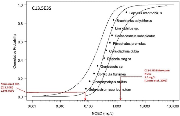
SSD based on chronic NOEC normalized to C_13.5E₃S and resulting HC₅. The data used to develop this distribution are given in Table 26. The mesocosm NOEC for C_12–15E₃S based on Lizotte et al. (2002) normalized to C_13.5E₃S is also shown for comparison.

Because there are no data on the acute or chronic toxicity of AES to sediment dwelling organisms, no PNEC for sediments could be estimated. Even so, given the relative lack of sorptivity of AES, it is reasonable to conclude that PNECs based on aqueous exposure would be protective of sediment dwelling organisms.

3. Bioconcentration factor

Due to AES's polarity, it is not expected to bioconcentrate in aquatic organisms. Experimental data confirm that AES is not bioconcentrated in fish. Kikuchi et al. (1980) conducted bioaccumulation studies in the common carp using ³⁵S-labeled C₁₂EO₃S and C₁₂EO₅S. Whole body BCFs (measured as ³⁵S residue) were 18 and 4.7 for C₁₂EO₃S and C₁₂EO₅S, respectively. Using ¹⁴C-C₁₄EO₂S, Dyer et al. (2009) determined metabolic clearance rates in subcellular liver fractions of the common carp and rainbow trout and cellular fractions of the carp and then used an in vitro to in vivo extrapolation model (Cowan-Ellsberry et al., 2008) to estimate whole-body clearance rates and BCFs. Predicted BCFs were 13.1 for both trout and carp using subcellular fractions whereas the predicted BCF for carp using hepatocyte cells was 10.3.

E. Linear Alkylbenzene Sulfonate

The toxicity of LAS has been widely investigated, and studies are available on acute, chronic, microcosm, mesocosm, and in situ exposures in the aquatic, and sediment environment. Compilations and summaries of these data are given in SDA (1991a), BKH (1993), OECD (2005), and HERA (2009a). The objective of this section is to summarize the toxicity of LAS and the relationship between the physical and chemical properties of LAS associated with toxicity and to describe how the PNEC which will be used in the prospective risk assessment was determined. A thorough summary of the toxicity of LAS is beyond the scope of this chapter, therefore the reader is recommended to go to the specific references for details on the toxicity studies cited.

1. Aquatic and sediment toxicity

A comprehensive review of the toxicity data for the aquatic compartment is found in BKH (1993) which contains 749 records of toxicity data for LAS covering several taxonomic groups and the SIDS assessment report (OECD, 2005). Intra and interspecies variability is large, particularly in the case of algae due to the fact that these toxicity values refer to different individual compounds and mixtures of isomers of LAS. Differences in test design as well as can account for some of this large range of species sensitivity.

The acute toxicity for commercial LAS is summarized in Table 27, where D. magna, P. promelas, and Lepomis macrochirus are chosen as representative organisms to illustrate the typical toxicity to invertebrates and fish. Data for algae refer to various species. The values in Table 27 are the geometric means of several studies, demonstrating the abundance of acute toxicity test data. These data are only for information because the abundance of higher tier data for LAS (i.e., chronic and mesocosm) means that these data are not required to determine the PNEC.

TABLE 27.

Aquatic acute toxicity for commercial LAS

Taxon	Geometric mean (mg/L)*
Algae	IC50 9.1 (n = 12, SD = ±3.9)
Aquatic invertebrate (D. magna)	EC50 4.1 (n = 17, SD = ±2.0)
Fish (Lepomis macrochirus)	LC50 4.1 (n = 12, SD = ±1.7)
Fish (P. promelas)	LC50 3.2 (n = 4, SD = ±1.6)

^*No. of records in parenthesis with standard deviations.

Source: Table 12 in HERA (2009a).

The chronic freshwater aquatic toxicity of LAS, based on effects on growth, survival, and reproduction, and evaluated in 19 different species with a broad taxonomic distribution, is summarized in OECD (2005). All the data in this summary are from studies judged to be “Reliable without restriction” (Klimisch values of 1) or “Reliable with restriction (Klimisch values of 2) based on criteria given in Klimisch et al. (1997). The details of the studies can be found in IUCLID5 entries in the Chemical Safety Report for the registered substance (LAS: 68411-30-3). This data set included algae, aquatic macrophytes, invertebrates, and fish. Photosynthetic organisms include blue-green and green algae as well as two floating aquatic macrophytes. Mollusks, water fleas, rotifers, and insects are representative invertebrates. Fish species include members of the salmonids, centrarchid, and cyprinid families and cover warm and cold water species. Across this large data set, the chronic aquatic toxicity to C_11.6LAS for the toxicity-weighted average structure (see Section V.E.2), ranged from 0.23 mg/L (rainbow trout) to 4.15 mg/L (Elimia, snail).

A variety of model aquatic ecosystem and mesocosm studies have been conducted on LAS. Many of these studies have been evaluated and summarized in two papers (Van de Plassche et al., 1999; Belanger et al., 2002). There is a substantial level of variability in the data among the 13 studies (Maki, 1981; Lewis, 1986; Lewis and Hamm, 1986; Huber et al., 1987; Fairchild et al., 1993; Lewis et al., 1993; Holt and Mitchell, 1994; Takamura, 1995; Tattersfield et al., 1995; Takamatsu et al., 1997; Jorgenson and Christoffersen, 2000; Belanger et al., 2002) with NOECs ranging almost 2.5 orders of magnitude, from 0.055 to 22.2 mg/L with an overall NOEC (mean ± 1 standard deviation) of 3.3 ± 6.04 mg/L. The extremes in the NOEC values are reported for lentic studies that were primarily conducted as single dose exposures. There was less variability in the NOECs when the test system was composed of lentic species and test solutions were renewed during the exposure (Maki, 1981; Huber et al., 1987). The structure and study design of the systems significantly impacts the study outcome because the lentic studies focused primarily on the autotrophic portion of the aquatic ecosystem. As reported by Fendinger et al. (1994) and van de Plaasche et al. (1999), algae are least sensitive and fish and invertebrates are similarly and more sensitive to anionic surfactants, such as LAS. Therefore, effects on autotrophs, which are the principal taxonomic group assessed in the lentic studies, would be observed at a higher concentration than for lotic studies that focused more on benthic fauna. In fact, lentic and lotic exposures had NOECs (mean ± 61 standard deviation) of 5.7 ± 67.64 and 0.53 ± 60.43 mg/L, respectively (Belanger et al., 2002). Belanger et al. (2002) conducted the most comprehensive study of LAS in aquatic stream mesocosms to date. Dodecyl LAS was dosed for 56 days, and microbial and invertebrate populations and communities were assessed. In addition, several species of invertebrates and fish were evaluated in cage enclosures in the flowing freshwater channels (Versteeg and Rawlings, 2003). An integrated mesocosm NOEC of 0.268 mg/L, adjusted for LAS bioavailability, was determined and reflected changes in stonefly, mayfly, and caddisfly species in exposed streams. The long-term comprehensive nature of the mesocosm study and its close reflection of natural systems have resulted in the direct use of the mesocosm NOEC in PNEC derivation (Versteeg et al., 1999; Belanger et al., 2002; OECD, 2005; HERA, 2009a).

Similar to the other surfactants, these aquatic toxicity data demonstrate that an increase in the chain length of LAS is associated with increases in toxicity. Increasing chain length causes an increase in the overall hydrophobicity of LAS, in conformity with the general observation that toxicity increases with increased hydrophobicity (Auer et al., 1990). Fendinger et al. (1994) observed an increase in toxicity of a factor of 2.7 for each increase in carbon number for fish and aquatic invertebrates due to increased hydrophobicity and increased uptake rate constants. Branching and the location of the phenyl position have also been associated with changes in toxicity due to changes in hydrophobicity (Roberts, 1988). For example, homologues with the same molecular weight (i.e., same number of carbons in the alkyl chain) but with a more terminal phenyl position (e.g., the 2-phenyl position) will be more toxic than homologues with a more central phenyl position (e.g., 5-phenyl position). This appears to be due to the intrachain carbon–carbon interactions which require fewer water molecules to solvate the alkyl chain leading to reduced hydrophobicity (Roberts, 1988). Similarly, branching on the alkyl chain causes reduced toxicity via a similar mechanism.

Three studies have been conducted that determine the toxicity of LAS to sediment organisms. The first study (Comber et al., 2006) determined the toxicity to freshwater sediment dwelling worms, Lumbriculus variegatus, using natural sediment with organic carbon content of 1.7% spiked with LAS. Exposure lasted 28 days, at which time the survival and change in biomass were determined. The EC₅₀ was ≥105 mg/kg sediment dry weight (dw). The NOEC was 81 mg/kg sediment dw. Significant degradation was measured over the 28-day duration of the study, equating to a half-life of 20 days in sediment. The second study (Comber et al., 2006) determined the toxicity to nematode species, Caenorhabditis elegans, using artificial sediment with organic carbon content of 2% spiked with C_11.4 LAS. Exposure lasted 3 days, at which time the survival and reproduction were determined. The NOEC for egg production was 100 mg/kg sediment dw, the NOEC for fertility was 200 mg/kg sediment dw, and the EC₁₀ for growth was 275 mg/kg sediment dw.

In the third toxicity study, Pittinger et al. (1989) exposed the filter and deposit feeding Chironomus riparius to natural stream sediments spiked with C_11.8 LAS and monitored midge emergence for approximately 24 days (until all midges emerged as adults). Emergence was significantly reduced at 993 but not at 319 mg/kg dw sediment. In 10-day survival and growth studies of L. variegatus exposed to C₁₂ 2-phenyl LAS, Mäenpää and Kukkonen (2006) reported NOECs in two different natural lake sediments of 344 and 510 mg/kg dw sediment. LOECs were 475 and 692 mg/kg dw. sediment. In both sediments, larval wet weight was a more sensitive indicator of toxicity than head capsule length. Body burdens at which effects occurred were 474 and 692 mg/kg of dw tissue.

2. Predicted No-Effect Concentration

In the aquatic environment, different homologues and isomers are present. The average alkyl chain length of LAS in the effluent of 15 activated sludge WWTPs is C11.8 (McAvoy et al., 1993). This value can be used as an environmental fingerprint in receiving water. However, because toxicity is not linearly related with chain length, the actual ecotoxicity of the environmental fingerprint is not the same as the ecotoxicity associated with this average structure. To take this into account, the toxicity-weighted average structure was calculated using the QSAR calculations (Köneman, 1981). This resulted in a toxicity-weighted average corresponding to a structure of C_11.6LAS. The ecotoxicity associated with a C_11.6 alkyl chain is, thus, expected to be representative of that of the overall LAS aquatic fingerprint in the aquatic environment.

To determine a single species-based PNEC, freshwater chronic toxicity values were normalized to C_11.6 LAS, and the method of van de Plaasche et al. (1999) was used to develop a SSD and estimate the HC₅. The freshwater SSD is plotted (Figure 5) as a cumulative distribution of normalized C_11.6 LAS chronic toxicity values for 20 taxa shown in Table 28. The 5th percentile value calculated from the SSD, the HC₅, was 0.21 mg/L (95th percentile confidence interval 0.059–0.402 mg/L). This single species HC₅ is at the low end of the range of model ecosystem NOEC values (0.055–22.2 mg/L), but similar to the NOEC from the most comprehensive model ecosystem study on C₁₂LAS, 0.268 mg/L. When corrected to a chain length of 11.6, the mesocosm NOEC is 0.395 mg/L. Given the duration of the mesocosm study, the rigor of the methods, diversity of species, and the need to assess effects at the community level, the mesocosm value of 0.395 mg/L is used as the definitive PNEC for risk assessment.

FIGURE 5.

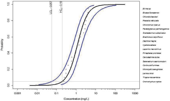
SSD for the full C_11.6 LAS data set (n = 19 taxa). The blue lines represent the 95% upper and lower confidence intervals of the regression. The predicted HC₅ of 0.19 mg/L is slightly less than the most sensitive species tested, rainbow trout, at 0.23 mg/L.

TABLE 28.

Original chronic NOEC for aquatic species to LAS. (In the seventh column, the toxicity values are reported as normalized to a single average environmentally relevant LAS structure (i.e., C_11.6). These geometric mean NOEC values will be used in the SSD (Figure 5) to represent that species.)

Taxon	Effect	Duration	End point	Original chain length	Original value (mg/L)	Normalized value (mg/L)
Fish
Lepomis macrochirus	Growth	30 days	NOEC	11.6	1.0	1.0
P. promelas	Survival	28 days	NOEC	11.8	0.90	1.09
P. promelas	Survival	196 days	NOEC	12	0.63	0.93
Geometric mean for P. promelas						1.0
O. mykiss	Growth	28 days	NOEC	11.6	0.43	0.43
O. mykiss	Growth	70 days	NOEC	11.6	0.23	0.23
O. mykiss	Growth	70 days	NOEC	11.6	0.32	0.32
Geometric mean for O. mykiss						0.32
Poecelia reticulata	Growth	28 days	NOEC	11.6	3.2	3.2
Tilapia mossambica	Reproduction	90 days	NOEC	11.6	0.25	0.25
Aquatic invertebrates
C. dubia	Reproduction	7 days	NOEC	11.8	0.5	0.61
C. dubia	Reproduction	7 days	EC10	11.8	0.99	1.20
Geometric mean for C. dubia						0.85
Chironomus riparius	Emergence	24 days	NOEC	11.8	2.4	2.91
D. magna	Reproduction	21 days	NOEC	11.8	1.18	1.43
D. magna	Reproduction	21 days	NOEC	11.8	2.19	2.66
Geometric mean for D. magna						1.95
H. azteca	Growth	32 days	EC20	12	0.95	1.40
Paratanytarsus parthenogenica	Survival	28 days	NOEC	12	2.0	2.94
Elimia sp	Growth	32 days	EC20	12	2.9	4.27
Brachionus calyciflorus	Reproduction	2 days	EC10	12.3	1.18	2.32
C. fluminea	Growth	32 days	EC20	12	0.27	0.40
Algae
Microcystis aeruginosa	Growth rate	96 hr	NOEC	11.9	0.30	0.40
Pseudokirchneriella subcapitata	Growth rate	96 hr	NOEC	11.9	0.50	0.67
D. subspicatus	Growth rate	72 hr	NOEC	11.6	2.4	2.4
D. subspicatus	Growth rate	72 hr	NOEC	11.6	0.4	0.4
Geometric mean for D. subspicatus						0.98
Chlorella kessleri	Growth rate	15 days	NOEC	11.6	3.0	3.0
Macrophytes
Elodea canadensis	Growth	28 days	NOEC	11.6	4	4
Lemna minor	Frond count	7 days	EC10	11.8	0.21	0.25

The PNEC for sediment can be derived from the chronic sediment toxicity data for the three species that represent different living and feeding conditions. To estimate the PNEC, an AF of 10 is applied to the lowest available NOEC value resulting in a conservative PNEC for sediment of 8.1 mg/kg dw sediment.

3. Bioconcentration Factor

LAS bioconcentration was studied employing a flow-through test system, in line with the OECD guidelines, using P. promelas as test fish (Tolls et al., 2000b). The test system used single homologue and isomer representatives of the commercial LAS to determine their uptake and elimination rates in fish. LAS reached a steady-state concentration in the fish body in about 3 days with biotransformation contributing more than 40% of the elimination for the C₁₂ 2-phenyl LAS homologue (Tolls et al., 2000b). BCF values were determined for each of the tested LAS homologues and isomers. The BCF values ranged from 2 L/kg for 6-phenyl C₁₀LAS to 990 L/kg for C₁₃ 2-phenyl LAS (Tolls et al., 1997). Using these values the BCF was estimated for the commercial LAS (C_11.6 alkyl chain length) and the environmentally representative average LAS of C_10.8 alkyl chain length. The BCFs were 87 L/kg and 22 L/kg, respectively, indicating that the bioconcentration potential of LAS is low and is decreased by environmental processes such as biodegradation and absorption (Tolls, 1998).

In addition, BCF was determined for P. promelas and three invertebrate species which were caged in streams during a C₁₂LAS model ecosystem experimental study (Versteeg and Rawlings, 2003). Total C₁₂LAS BCFs for these species ranged from 9 to 116 L/kg. In general, bioconcentration was affected by isomer position, exposure concentration, and species. BCF values tended to decrease as isomer position moved from external (e.g., 2-phenyl) to internal (e.g., 5,6-phenyl). BCFs also decreased as exposure concentration increased. BCFs for L. variegatus exposed to freshwater sediments spiked with the C₁₂ 2-phenyl LAS homologue were measured and found to be in the range of 0.5–4.7 L/kg depending on the sediment organic content (Mäenpää and Kukkonen, 2006).

VI. PROSPECTIVE RISK ASSESSMENT

To estimate the potential impact on the aquatic environment from each of the four surfactants and LCOHs, a prospective risk assessment is conducted. This prospective risk assessment calculates the ratio of the predicted surface water exposure concentrations (PEC) at the 90th percentile low flow and 90th percentile mean flow with the predicted no-effect concentration (PNEC) for each of the surfactants. This ratio (PEC/PNEC) is called the risk quotient. Values less than 1 indicate that there is a low potential for adverse effects in the aquatic environment because the predicted exposure concentration is less than the concentration that would not cause any adverse effects.

Table 29 summarizes the environmentally relevant structure for each of the chemicals and the calculated PNEC from Section V, as well as the exposure predictions from Section IV for this environmentally relevant structure. The risk quotient for each of the chemicals is below 1 for the aquatic environment. In fact, for most of the scenarios evaluated, the risk quotient is almost 2 orders of magnitude less than 1, indicating that the potential for any adverse effect on the environment from the use of these surfactants and LCOH as a result of dispersive release to the aquatic environment after wastewater treatment is very low.

TABLE 29.

Prospective risk assessment values; PNEC values came from Section Vand PEC values from Section IV

	Chemicals
	LCOH	AE	AS	AES	LAS
PNEC—predicted aquatic no-effect concentration (mg/L)
Environmental Relevant Structure	C13	C14.7EO9.1 (U.S.)	C13.6	C13.5E3S	C11.6
PNEC	0.0046	0.0983	0.039	0.076	0.21
PEC—predicted aquatic exposure concentration (mg/L)
90th percentile low flow	4.1 × 10−3	5.3 × 10−3	2.7 × 10−3	5.3 × 10−3	7.4 × 10−2
90th percentile mean flow	3.2 × 10−4	8.9 × 10−4	4.8 × 10−4	9.3 × 10−4	1.4 × 10−2
Risk quotient (PEC/PNEC)
Low flow	0.8913	0.0539	0.0692	0.0697	0.3524
High flow	0.0696	0.0091	0.0123	0.0122	0.0667

For most of these surfactants (i.e., AE, AS, and AES), the limited sediment toxicity data expressed as overlying water or pore water concentration shows that the risk assessment for the aquatic environment will protect the community of organisms that dwell in the sediment from adverse impact. Only LAS has a specific PNEC based on sediment concentration of 8.1 mg/kg dw sediment. The exposure concentration in the sediment can be calculated using the approach discussed in Section III.E. Using the 90th percentile low flow concentration of LAS predicted for the surface water (Table 13) of 7.4 × 10⁻² mg/L, a K_d value of 5360 L/kg for a C₁₂ 2-phenyl LAS (Belanger et al., 2002, in “Sorption” section in Section II.E.5) and the recommended defaults for surface water sediment concentration and sediment density (Section III.E), the sediment exposure concentration would be 7.3 mg/kg. Using the same 90th percentile low flow concentration for LAS, an organic carbon content of the sediment of 0.02 kg/kg, and a log K_oc of 4.83 for C₁₂ LAS (Traina et al., 1996, “Sorption” section in Section II.E.5), the sediment concentration would be 5.54 mg/kg. Thus, the risk quotient for sediments using these two exposure calculations would be 0.9 and 0.7, respectively. Both indicate that no adverse effect on the sediment dwelling organisms is expected.

In addition to the objective safety of these surfactants and LCOH in the aquatic and sediment environments, the BCFs for each of these chemicals are well below the regulatory concern levels of 2,000–5,000 (United Nations Environment Program [UNEP], 2001; European Commission, 2003). These regulatory concern levels indicate where a chemical could be considered “bioaccumulative” up the food chain such that the chemical could lead to toxic effects on higher trophic level organisms. Thus, in addition to no adverse effects upon direct contact with the surfactant in surface waters or sediments, there is no concern for any secondary effect of these surfactants on organisms that could be exposed to the surfactant through food.

VII. RETROSPECTIVE RISK ASSESSMENT USING MONITORING DATA

For chemicals that have been in commerce for an extended time, like the surfactants that are the subject of this paper, retrospective risk assessments can be done through comparison of chemical and biological environmental monitoring. Retrospective approaches require building an integrated assessment that provides a measure of the importance of the chemical discharges relative to other factors that can cause adverse biological responses. These other factors include in-stream habitat, and altered hydrology which impact the biological quality (e.g., structure and function). These factors, among others, occur in the ecosystem independently of the potential effects of the chemical. Because retrospective approaches evaluate the contribution of all of these potential causes of adverse impacts on the ecosystem, these approaches provide an ecological reality check by identifying which of the factors is a priority concern pertinent for appropriate management. Furthermore, a retrospective risk assessment can be used to verify and give confidence in the predictive risk assessment methods and to confirm the conclusions of prospective risk assessment. In order to conduct a retrospective risk assessment, there are several important factors to consider in choosing the site, designing the monitoring program, and conducting the analysis of the results.

A. Site Selection

When choosing sites for conducting the retrospective risk assessment for these surfactants, the ideal site would include a river that receives well-treated WWTP effluent, has little or no industrial discharges either to the water body or the WWTP, other stressors, natural habitat, low to minimal dilution, and is easily accessed for collecting samples. To choose sites that would meet as many of these criteria as possible, several pieces of information are required. These include:

• Information on the location of the discharge point(s) and quality and quantity of the effluent from the WWTP(s);

• Characteristics of the associated receiving water body. Characteristics of the water body of interest include the flow of the receiving water, depth, width, and substrate and stream/river bank quality;

• The presence of industrial discharges either directly to the water body or to the WWTP;

• Predominant type of land use around the water body, e.g., agricultural, urban.

This information can be obtained from a variety of sources such as satellite images, WWTP databases (e.g., U.S. EPA Clean Water Needs Survey and Permit Compliance System) and receiving water body characteristics (e.g., Enhanced Reach File 1, National Hydrography Dataset). Typically, these data are managed spatially via geographic information systems (GIS). Models such as iSTREEM® (Wang et al., 2000, 2005) can also be helpful as these integrate wastewater and receiving system attributes.

For example, in Sanderson et al. (2006a, 2006b), Atkinson et al. (2009) and Slye et al. (2011) studies, the monitoring sites were chosen based on the following criteria: (1) typical treatment efficiency (i.e., activated sludge); (2) wastewater influent that receives less than 10% industrial contributions; (3) low dilution (i.e., 7Q10 flow yielding dilution factors between 1 and 3) and (4) accessibility for sampling water, sediment, and biota. The presence of industrial contributions to domestic wastewater can both provide potential confounding chemical influences to wastewater treatment efficiencies as well as dilute the domestic sources of surfactants. Type II errors (i.e., accepting that there is no impact when an impact occurs) in field-based assessments are reduced by selecting low dilution sites. Hence the conclusions from the Sanderson, Atkinson, and Slye studies can be considered conservative. Another key attribute in site selection is an assessment of the physical habitat for aquatic fauna. For Sanderson et al. (2006a, 2006b), the RAPID bioassessment methodology by the United States Protection Agency (U.S. EPA, 1999) was used. For the Trinity River studies by Atkinson et al. (2009) and Slye et al. (2011), the Habitat Quality Index Score method was used (Texas Commission of Environmental Quality, 1999). Adequate habitat quality for fish and macroinvertebrates is essential for assessing the potential effects of chemicals. All useful habitat qualifications are based upon “reference conditions”. That is, there is an expectation that less human-altered habitats will yield the greatest potential for a diverse and highly functional ecological community. Sites that have reference-like qualities have the greatest potential to provide statistically significant relationships between chemical stressors and biological impacts (e.g., greatest signal to noise ratio). However, if insufficient habitat exists, then relationships of chemical measurements in the aquatic and/or sediment compartments to biological impacts will be confounded.

B. Monitoring Study Design

The second component of designing a retrospective assessment is to have a well-designed and executed monitoring program that provides information not only on the chemical(s) of interest but also on other potential stressors and the biological community status of the receiving water body. The subsequent paragraphs represent a synthesis of several surfactant monitoring studies, including Sanderson et al. (2006a, 2006b), Atkinson et al. (2009), and Slye et al. (2011).

The surfactant monitoring at each of the selected sites should consist of samples of WWTP influent and/or effluent, and upstream and downstream samples of the receiving water and sediments. Typically composite samples of influent are used to average out fluctuations during the day. Due to the hydrologic retention period of most WWTPs, a grab sample of effluents is typically sufficient. The number of upstream and downstream samples depends on the goals of the study and especially on whether the sites are on a single water course. At least one sample of water and sediment should be taken upstream of the first WWTP discharge to allow for characterization of background conditions. Other sample locations are located downstream of effluent mixing zones to ensure complete mixing of the effluent and the receiving water. Sediment sampling should be biased towards areas of fine, recently deposited sediments, since these are most likely to contain surfactants and other chemicals of interest. Sediment samples should be taken from the upper 5–10 cm depth and from several locations in the deposition zone and composited. The composited samples would be centrifuged to remove the porewater which should also be analyzed for water chemistry and the surfactant of interest. The surfactant samples should be preserved with 8% v/v formalin (or another preservation scheme that is deemed adequate) within minutes after collection in the field to ensure that the samples do not lose associated surfactants due to biodegradation.

In addition to the surfactants, the monitoring studies should include other chemicals to allow for determining if other stressors may be present. Therefore, all samples that are collected (i.e., effluent mixing zone, upstream and downstream receiving water and sediments) should be analyzed for general water chemistry, key ionic constituents, nutrients and trace elements as given in Table 30, using the appropriate analytical methods. Understanding of conventional pollutants, such as BOD and ammonia, provides an indication of how well the WWTP are performing at the time of the study. Poor performance of a WWTP could confound relationships to biological impacts. Habitat and physical/chemical field data should be collected at each sampling location in order to conduct a habitat assessment (e.g., Chapman and Anderson, 2005; Sanderson et al., 2006b). The parameters measured for the Trinity River studies are given in Table 31 (Atkinson et al., 2009). Each parameter is scored according to a predefined algorithm, and the scores are summed for an overall index of quality for each transect. These habitat parameters are useful in determining Habitat Quality Index Score that indicates if there have been beneficial or detrimental effects to vertebrate and invertebrate fauna. For example, the Habitat Quality Index Score established by the Texas Commission of Environmental Quality (1999) are based on nine parameters: available instream cover, bottom substrate stability, number of riffles, dimensions of largest pool, channel flow status, bank stability, channel sinuosity, riparian buffer vegetation, and esthetics of reach. Each parameter is rated according to predefined scoring categories (potential scores range from 0 to 4), and then the nine scores are summed for an overall index of quality for each sampling site. Theoretically, the HQIS can range from 4 to 31 with the higher scores indicating a higher quality habitat.

TABLE 30.

Analytical analyses typically conducted on water and sediment samples with methods indicated

Field parameters	Laboratory parameter
Sediment
Texture	Moisture content (ASTM D2216)
Redox potential	Bulk density (ASTM C127)
pH	Grain size (ASTM D422)
	Total organic carbon (EPA 415.1)
	Total sulfide (EPA 376.1)
	Organic matter content (ASTM 2974)
	Kjeldahl nitrogen (EPA 351.2)
	Total phosphorous (EPA 365.1)
	Atterberg limits (ASTM D4318)
	Cation exchange capacity (EPA SW846 9080)
Surface water
Temperature	Total dissolved solids (EPA 160.1)
Dissolved oxygen	Total organic carbon (EPA 415.1)
Turbidity	Biological oxygen demand (EPA 405.1)
Redox potential	Chemical oxygen demand (EPA 401.1)
Salinity	Hardnesss (EPA 130.1)
Conductivity
pH
Sediment porewater
Temperature	Total dissolved solids (EPA 160.1)
Dissolved oxygen	Total organic carbon (EPA 415.1)
Redox potential	Biological oxygen demand (EPA 405.1)
Salinity	Chemical oxygen demand (EPA 410.1)
Conductivity	Hardness (EPA 130.1)
pH

TABLE 31.

Habitat and physical/chemical parameters collected on the Trinity River

Substrate
Pool substrate type(s)	Variability in pool substrate type
Sediment deposition rate	Substrate stability
Channel
Longitude and latitude	Width and depth profile
Flow status and rate	Extent of anthropogenic alteration
Sinuosity	Number of riffles
Dimension of pools	Esthetics of reach
Bank
Stability and slope of bank	Presence of vegetation
Vegetative zone width	Vegetation types
Extent of in-stream cover	Adjacent land use

Biological monitoring for the invertebrate and vertebrate fauna should be included to determine the ecological status at the sites. Status can be expressed in a myriad of ways, including species richness, evenness, ecological functional groups, and pollution tolerance. Macroinvertebrate community monitoring can be conducted via direct sampling such as D-frame dip net, or by artificial substrates. Artificial substrate samplers should be placed in depositional areas and to the extent possible arranged in similar substrate types along the course of the river, downstream from the WWTPs. Another a common method used to collect benthic invertebrates is a D-frame dip net (650 μm mesh size), which is jabbed into the sediment across each stream. The number of jabs for each habitat type would be proportional to habitat types present in each location. Samples should be collected from similar habitats at each location at each stream. Each sample should be placed in plastic jars, preserved with ethanol, and stored for identification and enumeration in the laboratory.

C. Analysis of the Monitoring Data

Ascertaining ecological status or impacts requires comparison to a “reference site or condition”. Reference sites are typically minimally affected by humans, therefore providing an expectation of what “should be” found in a similar habitat. If no differences in biological status are found at sites downstream of WWTPs, as compared to reference sites, then it can be concluded that these surfactants as well as other chemicals that co-emanate from the selected wastewater discharge site do not adversely affect ecological status and, therefore, do not cause concern. The relative confidence of such conclusions and their application to non-monitored sites will be based upon the quality of the site selection. However, once it is determined that the state of the water body is less than that expected by the reference condition and the degree to which it is impacted, the next step is to determine the cause or causes for this reduction in state before any attempt is to be made to develop or implement remediation or environmental management action. A framework for relating measured biological impacts to the presence of potential chemical mixtures has been described by ECETOC (2011) and is shown in Figure 6.

FIGURE 6.

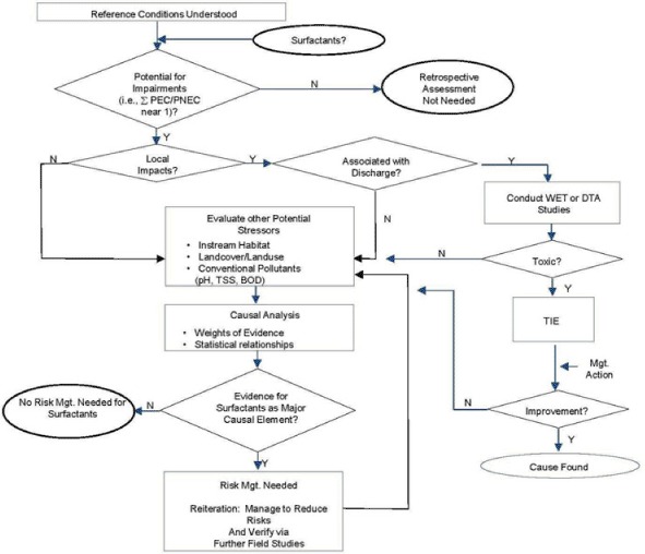
Suggested approach to assessment of ecologic risk of mixtures of chemicals in the aquatic environment.

The summations of exposures of surfactants described in this review have the potential to exceed an additive PNEC. Consequently, it is important that prospective approaches, as described in Section VI, be verified via field studies. Figure 6 illustrates the potential analysis options when conducting a retrospective field study on surfactants. Given the high volume of these chemicals, it is reasonable to assume that only a direct comparison of PEC/PNEC ratios to biological community status downstream of a given WWTP will provide sufficient evidence to indicate that a risk retrospective assessment is not needed. On the contrary, because surfactants are discharged from thousands of WWTPs in North America, a retrospective study of surfactants should be considered on a multisite, even a river basin-based scale. As illustrated in Figure 6, the primary analysis option is to consider potential effects to be dispersive in nature not localized. If in the analysis surfactants are found to be associated with localized impacts, further verification could be pursued via traditional whole effluent toxicity or directed toxicity assessment approaches followed by appropriate risk management schemes. However, given that whole effluent studies typically indicate that surfactants are not a primary cause of toxicity, other analysis methods are needed to more fully assess the potential effects. These methods need to include potentially cooccurring stressors associated with effluent discharge, such as conventional pollutants, local in-stream habitat alterations, and hydrological and chemical perturbations caused by changes in land-use and land-cover (e.g., urbanization). In essence, these field studies require methods that will allow the relative effect of the surfactants relative to other stressors to be evaluated. Relative causality can be established via statistical as well as WoE approaches. If the exposure to surfactants provides a relatively low weight compared to that of other stressors with regard to measured in-stream biological impacts, or lack of impact, then it can be reasonably concluded there is no need for surfactant mitigation efforts. However, if there is an impact, management of other chemicals or nonchemical stressors may be required.

D. Review of Retrospective Risk Studies

Sanderson et al. (2006b) conducted a WoE risk assessment in three streams in Ohio and Indiana. The team developed a WoE assessment methodology as described previously. Biota and habitat information was collected to ground-truth the predicted risk levels within field assessments and to correlate the collected variables. Each variable constituted a line-of-evidence (LoE) which was summarized in a WoE analysis. This information was used to test different hypotheses—e.g., regarding risks from surfactant exposure. Evaluation of surfactant risks in surface water and sediments required the assessment of surfactant exposure, presence of other environmental stressors and statistically relate these to biological community condition—hence, a complex analysis (Dyer and Wang, 2002). A framework for considering all data associated with the potentially perturbed locations warranted a WoE approach. Chapman and Anderson (2005) provided a comprehensive and pragmatic framework for assessment of sediment contamination on a WoE basis. Since the Sanderson et al. (2006b) study focuses on the perturbation and risk of a few constituents (surfactants) from municipal WWTPs, it is appropriate to adapt and combine the Chapman and Anderson (2005) decision matrix for WoE categorization with the U.S. EPA (1999) RAPID bioassessment method for assessment of environmental perturbation and risk of surfactants in streams. Sanderson et al. (2006b) defined a 20% and 50% alteration of benthos (relative to the total mean or upstream abundance) as significant using both the RAPID and Chapman and Anderson (2005) methodologies. That is, upstream of the WWTP served as the reference condition in this approach. Ecological status was determined by examining species richness and percent EPT (i.e., Ephemeroptera sp., Plecoptera sp., and Trichoptera sp.) taxa as a community quality compositional measures; percent tolerant taxa as a measure of tolerance to perturbation; and percent clingers as a measure of sediment habitat quality. The toxicity statement was substituted with a risk expression based on the measured environmental concentrations divided by the PNEC, plus the biomagnification potential of the compound as suggested by Chapman and Anderson (2005). Chapman and Anderson's (2005) three ordinal ranking levels were adapted to achieve a semiquantitative analysis (0, 1, and 2), which could then be summed across various LoE.

Atkinson et al. (2009) and Slye et al. (2011) conducted a retrospective risk assessment study on the Trinity River in Texas. The Trinity River system has been extensively studied. In fact, a major survey was conducted in 1987 to 1988 by the University of North Texas (UNT) Institute of Applied Sciences (IAS) (“A Water Quality and Ecological Survey of the Trinity River” conducted for City of Dallas Water Utilities, 1989). For the past 20 years, benthic macro-invertebrate community structure studies have been conducted on the upper Texas Trinity River, USA, which is dominated by municipal WWTP and industrial effluents. The Trinity River in North Central Texas flows through the highly populated Dallas-Fort Worth (DFW) metroplex area and is typical of many urban rivers in the Southern United States that have flows dominated by input from WWTPs. As such, the Trinity River represents a near-worst-case scenario and presents an opportunity to examine the environmental effects of domestic-municipal and industrial effluents on aquatic life.

The Trinity River studies indicate that many stretches of the river support a diverse benthic community structure (Slye et al., 2011); however, a decline in taxa richness occurred immediately downstream of WWTPs. Furthermore, these studies show the PEC/PNEC ratios for surfactants to be below unity, indicating that there is little evidence to suggest that surfactants are a primary driver of receiving water ecological status. This conclusion was verified via regression modeling, where benthic macroinvertebrate metrics were not correlated with surfactant levels. However, surface water surfactant levels may act as surrogates to other potential stressors emanating from WWTPs, as multiple linear regression modeling indicates that surfactant toxic units were often found within the top three factors associated with various aspects of ecological status.

Another retrospective study (De Zwart et al., 2006) is an ecoepidemiological assessment of several metals, ammonia, and chemicals from household products, including AS, AES, AE, and LAS, at 695 sites in the state of Ohio. This study combined several existing databases using GIS software. The baseline river mapping data for Ohio came from the U.S. EPA's reach file Version 1 (RF1) (U.S. EPA, 1992). This was then combined with fish survey data by location provided by the Ohio Environmental Protection Agency (Ohio EPA), Columbus, Ohio, USA, for 98 native and 19 introduced fish species (Trautman, 1981; Barbour et al., 1999) for the years 1990–1996. Local, site-specific, fish habitat data by location was also provided by the Ohio EPA. Habitat data included sampling location (latitude, longitude), drainage area above each sample site, and the individual metrics used to derive Ohio EPA's qualitative habitat evaluation index (QHEI; Rankin, 1989). Ambient water-chemistry data for Ohio streams from U.S. EPA's STORET database (U.S. EPA, 1995). Parameters were total metal concentrations (Cd, Cu, Pb, Ni, Zn), dissolved oxygen, hardness, total ammonia, pH, and total suspended solids for the years 1990–1996, the same time period over which data on fish assemblages were compiled. The median and 90th-percentile concentrations for each water-chemistry parameter were determined per site from these data. Using mean flow data for all receiving waters from U.S. EPA's RF1 river file (U.S. EPA, 1992) and flow data obtained from municipal WWTPs, the cumulative percentage WWTP effluent as a surrogate measure of persistent wastewater constituents within stream reaches was estimated. The GIS-ROUT model (Dyer and Caprara, 1997; Wang et al., 2000, 2005), which is the precursor to the iSTREEM® model, was used to estimate riverine concentrations of chemicals derived from household products.

Using SSDs for the metals, ammonia and the chemicals in household products, the potentially affected fraction (PAF) of species at a given concentration was estimated for each particular site, these values were then added to derive msPAF (multi substance) values for the sites. The identification of sites with impairment involved comparing the biological condition from the fish survey data with predictions from RIVPACS-type models (Moss et al., 1987; Hawkins, 2006), which estimates the aquatic fauna expected to occur in the absence of (or minimal) human-caused stress. Statistically significant associations between impacts on species abundances and stressor variables, represented by the PAF values, were used to identify likely causes of biological impairment.

Of the 695 sites assessed, De Zwart et al. (2006) showed that 3% of adverse effects to Ohio fish communities could be associated with down-the-drain product chemicals. In comparison, the presence of municipal effluent (3%) altered habitat (16%) and water chemistry (28%) were associated with impacts to fish community status.

The relatively minor contributions of down-the-drain chemicals determined in the Trinity River and Ohio studies are further verified by Dyer and Wang (2002), where they used simple t-tests to determine upstream to downstream differences in macroinvertebrate and fish communities. No significant differences in macroinvertebrate and fish community status were observed in rural environments.

Therefore, considering all the retrospective studies mentioned above, there is little evidence to suggest that surfactants as a whole (e.g., mixture) are primary stressors on receiving water ecological communities which supports the conclusions of the prospective risk assessment (Section VI).

VIII. KEY SCIENTIFIC ADVANCES

The environmental risk assessment of surfactants described in this paper would not have progressed as far as it has without the development of key technologies. The most important areas of the risk assessment are development of exposure data and toxicological information to derive the PEC/PNEC ratios and thus a risk factor. In the absence of measured data, advances in our predictive capabilities for exposure and effects have significantly reduced the uncertainty associated with evaluating chemical risk in the aquatic environment.

Development of the environmental exposure is premised upon the ability to measure surfactant and surfactant components in environmental media. In early days of study, surfactant analytical methods used colorimetric indicators, such as CTAS for AE (nonionics) and MBAS for AES and LAS (anionics). The earliest documented methods for MBAS date back to the late 1950s and 1960s with the Association of American Soap and Glycerine Producers (Sallee et al., 1956; Weaver and Coughlin, 1960), which would become The SDA in the 1960s. The detection limits for total surfactants using these methods were approximately 0.5 mg/L, and these values could have been compromised by matrix interactions and environmental contamination. As the need for lower detection limits arose, new methods emerged that increased sensitivity. These methods still lacked specificity, for example, the hydrogen bromide derivitization method for measuring alcohol-based surfactants by Fendinger et al. (1995). Therefore, methods quickly evolved including LC ELSD (liquid chromatography—evaporative light scattering detection), which lowered detection limits to approximately 500 μg/L. This technique was still not sensitive enough for deriving a PEC/PNEC (Dubey et al., 1995) because environmental concentrations were much lower. To detect surfactants in the low ppt (ng/L) concentration range, more sophisticated technologies were developed using thermospray LC/MS (Evans et al., 1994; Popenoe et al., 1994) and later LC/MS with derivitization by pyridinium methods (Dunphy et al., 2001). These methods allowed for ppt (ng/L) levels of quantitation. For example, low ppt concentrations of AE could now be detected in the environment, and individual homologues could be identified and quantified. The number of homologues for AE is quite large. For example, C_12–15AE with an average of 7 ethoxylate groups would have a distribution of C₁₂, C₁₃, C₁₄, and C₁₅ chain lengths, each with a distribution of ethoxylation from EO₀ to EO₂₁. For this example, the number of homologues could be greater than 88. These later methods enable a “fingerprint” of these homologues to be developed.

Significant improvements were also achieved in our ability to measure fate parameters in wastewater, activated sludge, and aquatic environments. Advanced methods for biodegradation testing including the shake flask test and semiCAS procedure (SDA, 1965) became approved international methods (i.e., ASTM International D2667-95; OECD 301, 302 and 303 guidelines). The most important advances were facilitated by advances in radiolabel (¹⁴C) synthesis and analysis of parent compounds. For example, the use of LC-and TLC-RAD techniques to measure parent compounds at extremely low concentrations allowed for more accurate determinations of biodegradation rate constants (Steber and Wierich, 1987; Steber et al., 1988; Nuck and Federle, 1996; Nielsen et al., 1997; Itrich and Federle, 2004; Federle and Itrich, 2006) and sorption coefficients (Kerr et al., 2000; McAvoy and Kerr, 2001; van Compernolle et al., 2006).

In addition to improved laboratory testing methodologies, better predictive mathematical models were developed for assessing the fate and transport of surfactants in activated sludge treatment and receiving waters. For example, the ASTreat model (Lee et al., 1998; McAvoy et al., 1999) has been successfully used to predict effluent concentrations of surfactants in activated sludge treatment and the iSTREEM® model (Wang et al., 2000, 2005) was used in this paper to predict receiving water exposure concentrations of LAS, AE, LCOH, AS, and AES in U.S. rivers. Accurate fate data are needed for predicting exposure concentrations in aquatic environments, thus improvements in the fate laboratory testing methods has also improved our predictive capabilities.

The improvements in analytical chemistry for quantification of surfactant concentration and homologues have also facilitated the development of higher-order toxicity testing. Laboratory toxicity testing methods were improved because acute tests in 24–96 hr exposures were found inadequate for estimating environmental toxicity of surfactants at low ppb concentrations. Chronic laboratory methods were modified to enable testing of readily biodegradable surfactants with half-lives (DT₅₀) from a few days to less than 1 day. Morrall et al. (2003), for example, evaluated several AE in chronic, flow-through 21-d D. magna studies where renewal frequency was titrated to account for losses due to degradation balanced against flow rates suitable for Daphnia health. Dosing techniques were developed for highly insoluble materials and those that were readily biodegradable. The analytical development mirrored the toxicity testing development to provide chronic exposures for many species using measured concentrations. However, closer to field exposures were desired to further quantify environmental effects of surfactants. Flowing water experiments in artificially derived indoor and outdoor streams (mesocosms) were developed so as to expose in situ biological communities natural to an area to a quantified dose and concentration of surfactant. The mesocosms allowed algae, macrophysics, stream invertebrates, fish and amphibians of different life stages to be exposed under controlled surfactant exposures allowing for replication and exposure series of carefully dosed chemicals that were fingerprinted to describe exposures (Belanger, 1992; Belanger et al., 1994; Rodgers et al., 1996; Association Internationale de la Savonnerie et de la Detergence [AISE] & Comité Européen des Agents de Surface et leurs Intermédiaires Organiques [CESIO], 1995).

To better describe the effects side of the risk equation, QSARs were developed for many taxa in experimental systems in single species experiments up to complex multispecies mesocosm systems and could be quantified for the specific homologues mixture identified using LC/MS techniques. Class-specific acute and chronic toxicity QSARs were developed for alcohols (Fisk et al., 2009; Schäfers et al., 2009), AS (Dyer et al., 1997), AES (Dyer et al., 2000), AE (Gillespie et al., 1999; Lizotte et al., 1999; Boeije et al., 2006; Wind & Belanger, 2006; Wong et al., 1997), and LAS (Fendinger et al., 1994). Other structure–activity-related developments included advancements relative to biodegradation (Federle and Itrich, 2006) and sorption (van Compernolle et al., 2006).

Toxicity QSARs were developed for many species, and those results could be further refined in SSD to derive a chronic concentration for the populations (HC₅). This approach, initially explored in van de Plaasche et al. (1999), was limited at the time due to gaps in toxicity data and complete knowledge of environmental fingerprints. Homologue-specific monitoring and experience has refined how this approach can be used for environmental risk assessment, which is exemplified by AE (Belanger et al., 2006).

The QSAR developments allowed the use of homologue fingerprint to predict the toxicity in an environment from environmental samples taken from either a discharge effluent or in a water body. In fact, the QSAR could predict the “bioavailable” fraction of the homologues by accounting for sorption to particles in solution within the wastewater stream or water body. This ability to use a fingerprint to predict toxicity from QSAR(s) of species or species distributions modified for sorption to particles enabled refinement of the AF that had been used in past assessments. The use of AF was believed to account for toxicological uncertainty between acute and chronic, chronic and mesocosm as well as interspecies differences. Using fingerprint specific, HC₅ distributions and site factors (e.g., accounting for reduced bioavailability due to solids in solutions), an AF of 1,000 typically used to estimate toxicity to in stream concentrations could be significantly reduced. In addition, these studies supported the refinement of the AF based on the level of data available (i.e., acute, chronic, and mesocosm) resulting in a more realistic risk prediction of surfactants in the environment.

The chemicals described in this paper are all HPV chemicals with tonnages well above 1,000 tons per year, and are included in the voluntary HPV programs of the U.S. EPA and the OECD. Policy makers recognize that the assessment and regulation of chemicals globally is best accomplished by assessing categories of chemicals, rather than individual chemicals, whenever possible. The surfactant industry has conducted and submitted some of the largest HPV category assessments, both in terms of CAS#s and tonnage in the world. These assessments serve as examples of how category assessments can be successfully conducted under emerging chemical regulations, e.g., REACH. One of the best illustrations of this category approach is that of the OECD assessment of the long-chained aliphatic alcohols (OECD, 2006). Moreover, in developing this category assessment, the LCOHs challenged the science and current toxicity and biodegradation test methods in a number of ways, e.g., how to conduct chronic testing of a very rapidly degraded/metabolized compound up to and beyond their solubility? These challenges and their solutions were described in a special issue of Ecotoxicology and Environmental Safety (2009; vol. 72). Once these challenges were met, the next challenge from a risk perspective was the environmental forensic sorting of the surfactant contribution of LCOH from LCOH coming from natural sources as well as understanding the contribution of in-stream loss of LCOH versus LCOH formed from degradation and in situ de novo synthesis. How these challenges were addressed and overcome is described in Mudge et al. (2010, 2012).

Ground-truthing of environmental risk assessment results in the environment is a difficult endeavor, especially for chemicals with wide-dispersive use such as the detergent surfactants discussed in this paper. For this reason, the science of eco-epidemiology was pioneered. The goal of eco-epidemiology is to develop a WoE ecological approach that can be used to determine the relative contributions of down-the-drain chemicals and all other stressors to environmental impacts observed in receiving environments. The relative contributions can be used to identify the degree to which down-the-drain consumer product ingredients contribute to the ecological status and quality downstream of wastewater treatment facilities in the context of all other potential stressors and whether any risk management actions are required. The papers cited in Section VII (Dyer and Wang, 2002; De Zwart et al., 2006; Sanderson et al., 2006a, 2006b; Atkinson et al., 2009; Slye et al., 2011) describe and have contributed to the development of this methodology.

IX. SUMMARY AND CONCLUSIONS

The Association of American Soap and Glycerine Producers first started to study and make publicly available the environmental fate and hazards of synthetic surfactants in the 1950s to understand the potential for environmental effects associated with their usage. Successor organizations, including The SDA and the ACI, have continued the commitment to ensure that high-quality data and risk assessments are available in order to illustrate the environmental safety of surfactants, and continuously improve the sustainability of the industry and the transparency of data.

This paper summarizes over 250 published and unpublished studies on the environmental properties and impacts of the four major, high-volume surfactant classes (AS, AE, AES, and LAS) as well as the linear alcohol feedstock (LCOH). To date, this is the most comprehensive report on these surfactants’ chemical structures, use and volume information, physical/chemical properties, and environmental fate properties such as biodegradation and sorption. Moreover, this compilation includes a review of the most relevant surfactant monitoring studies through sewers, WWTPs and eventual release to the environment. Further, this paper includes a comprehensive summary of aquatic and sediment toxicity information, drawing from fish, algae and microorganism acute and chronic toxicity studies and numerous stream mesocosm assessments for the surfactant categories.

These data are then used in the paper to illustrate the process for conducting both prospective and retrospective risk assessments for large-volume chemicals and categories of chemicals with wide dispersive use. The prospective assessment approach builds on a thorough understanding of the processes that lead to release of these types of chemicals into the aqueous environment, and the fate of the chemical along this fate train. The surfactant and cleaning products industry has devoted many years and countless resources in understanding, for example, how wastewater treatment processes effect the fate and eventual release to surface waters of a chemical in WWTP effluents. In addition, the industry has developed and conducted necessary monitoring and in situ studies to demonstrate how a retrospective assessment can be used to refute or validate the conclusions of prospective risk assessments. Through these efforts, the detergent industry has been able to improve the risk assessment process and result in more confidence in the assessment process.

This paper also highlights the many years of research that the surfactant and cleaning products industry has supported to improve environmental analytical and testing methods, many of which have become approved international standard methods. From the SDA shake culture test and semi CAS procedure to determine surfactant biodegradability which were developed in the 1960s for tracing detergent alcohols through the environment via stable isotope labeling in 2010, this industry has been at the forefront of designing and refining analytical methods for environmental monitoring and testing. Similarly, the industry has improved animal test methods, including flow-through systems for degrading chemicals to enable chronic aquatic toxicity testing as well as advancing mesocosm assessment methods and approaches. Finally, the industry has supported the advancement of innovative environmental models. QSAR, PEC/PNEC ratios, iSTREEM® have all been developed through surfactant research. These key tools, approaches, methods and research findings have been shared with the wider chemical community as part of the efforts to promote responsible chemical stewardship globally. This thorough review and the resulting prospective risk assessments of AS, AES, AE, and LAS have demonstrated that these surfactants and the long-chain linear alcohols, LCOH, although used in very high volume and widely released to the aquatic environment, have no adverse impact on the aquatic or sediment environments at current levels of use. The retrospective risk assessments of these same chemicals have clearly demonstrated that the conclusions of the prospective risk assessments are valid and confirm that these surfactants do not pose a risk to the aquatic or sediment environments. The supporting data as well as the resulting prospective and retrospective risk assessments demonstrate the industry's environmental sustainability commitment, “To only market products that have been shown to be safe for humans and the environment, through careful consideration of the potential health and environmental effects, exposures and releases that will be associated with their production, transportation, use and disposal.”

REFERENCES

- Aldenberg T., Slob W. Confidence limits for hazardous concentrations based on logistically distributed NOEC toxicity data. Ecotoxicol. Environ. Saf. 1993;25:48–63. doi: 10.1006/eesa.1993.1006. [DOI] [PubMed] [Google Scholar]
- Aldenberg T., Jaworska J. Uncertainty of the hazardous concentration and fraction affected for normal species sensitivity distributions. Ecotoxicol. Environ. Saf. 2000;46:1–18. doi: 10.1006/eesa.1999.1869. [DOI] [PubMed] [Google Scholar]
- Association Internationale de la Savonnerie et de la Detergence [AISE] & Comité Européen des Agents de Surface et leurs Intermédiaires Organiques [CESIO] Environmental risk assessment of detergent chemicals. Proceedings of the AISE/CESIO Limelette III workshop. 1995, November:73. Retrieved from: http://www.erasm.org/workshop.htm. [Google Scholar]
- Atkinson S. F., Johnson D. R., Venables B. J., Slye J. L., Kennedy J. R., Dyer S. D., Price B. B., Ciarlo M., Stanton K., Sanderson H., Nielsen A. Use of watershed factors to predict consumer surfactant risk, water quality, and habitat quality in the upper Trinity River, Texas. Sci. Total Environ. 2009;407:4028–4037. doi: 10.1016/j.scitotenv.2009.02.029. [DOI] [PubMed] [Google Scholar]
- Auer C. M., Nabholz J. V., Baetcke K. P. Mode of action and the assessment of chemical hazards in the presence of limited data: Use of Structure-Activity Relationships (SAR) under TSCA, Section 5. Environ. Health Perspect. 1990;87:183–197. doi: 10.1289/ehp.9087183. Retrieved from http://www.ncbi.nlm.nih.gov. [DOI] [PMC free article] [PubMed] [Google Scholar]
- Barbour M. T., Gerritsen J., Snyder B. D., Stribling J. B. Rapid bioassessment protocols for use in streams and wadeable rivers: Periphyton, benthic macroinvertebrates and fish (2nd Ed) Washington, DC: U.S. EPA, Office of Water; 1999. Retrieved from: http://water.epa.gov/scitech/monitoring/rsl/bioassessment/index.cfmEPA 841-B-99-002. [Google Scholar]
- Battersby N. S., Kravetz L., Salanitro J. P. Proceedings of 5th CESIO World Surfactant Congress. Fienze: Fortezza da Basso; 2000. Effect of branching on the biodegradability of alcohol-based surfactants; pp. 1397–1407. [Google Scholar]
- Battersby N. S., Sherren A. J., Bumpus R. N., Eagle R., Molade I. K. The fate of linear alcohol ethoxylates during activated sludge treatment. Chemosphere. 2001;45:109–121. doi: 10.1016/S0045-6535(01)00030-3. [DOI] [PubMed] [Google Scholar]
- Belanger S. E. Use of experimental stream mesocosms to assess ecosystem risk: A case study with a cationic surfactant. In: Cairns J. Jr., Neiderlehner B. R., Orvos D. R., editors. Predicting ecosystem risk. New York, NY: Princeton Scientific Publishing Company; 1992. pp. 263–287. [Google Scholar]
- Belanger S. E. Literature review and analysis of biological complexity in model stream ecosystems: Influence of size and experimental design. Ecotoxicol. Environ. Saf. 1997;36:1–16. doi: 10.1006/eesa.1996.1487. [DOI] [PubMed] [Google Scholar]
- Belanger S. E., Barnum J. B., Woltering D. M., Bowling J. W., Ventullo R. M., Schermerhorn S. D., Lowe R. L. Algal periphyton structure and function in response to consumer chemicals in stream mesocosms. In: Graney R. L., Kennedy J. M., Rodgers J. R., editors. Aquatic mesocosm studies in ecological risk assessment. Boca Raton, FL: SETAC Special Publication Series, Lewis; 1994. pp. 535–568. [Google Scholar]
- Belanger S. E., Bowling J. W., Lee D. M., LeBlanc E. M., Kerr K. M., McAvoy D. C., Christman S. C., Davidson D. H. Integration of aquatic fate and ecological responses to linear alkyl benzene sulfonate (LAS) in model stream ecosystems. Ecotoxicol. Environ. Saf. 2002;52:150–171. doi: 10.1006/eesa.2002.2179. [DOI] [PubMed] [Google Scholar]
- Belanger S. E., Dorn P. B. Burridge L. E., Haya K., Niimi A. J., editors. Chronic aquatic toxicity of alcohol ethoxylates (AE) surfactants under Canadian exposure conditions. Proceedings of the 31st annual aquatic toxicity workshop: October 24 to 27. Can. Tech. Rep. Fish. Aquat. Sci. 2004;2526:95–104. [Google Scholar]
- Belanger S. E., Dorn P. B., Toy R., Boeije G., Marshall S. J., Wind T., Van Compernolle R., Zeller D. Aquatic risk assessment of alcohol ethoxylates in North America and Europe. Ecotoxicol. Environ. Saf. 2006;64:85–99. doi: 10.1016/j.ecoenv.2005.11.003. [DOI] [PubMed] [Google Scholar]
- Belanger S. E., Guckert J. B., Bowling J. W., Begley W. M., Davidson D. H., LeBlanc E. M., Lee D. M. Responses of aquatic communities to 25-6 alcohol ethoxylate in model stream ecosystems. Aquat. Toxicol. 2000;48:135–150. doi: 10.1016/S0166-445X(99)00048-X. [DOI] [PubMed] [Google Scholar]
- Belanger S. E., Lee D. M., Bowling J. W., LeBlanc E. M. Responses of periphyton and invertebrates to tetradecyl-pentadecyl sulfate mixture in stream mesocosms. Environ. Toxicol. Chem. 2004;23:2202–2213. doi: 10.1897/04-49. [DOI] [PubMed] [Google Scholar]
- Belanger S. E., Meiers E. M., Bausch R. G. Direct and indirect ecotoxicological effects of alkyl sulfate and alkyl ethoxysulfate on macroinvertebrates in stream mesocosms. Aquat. Toxicol. 1995a;33:65–87. doi: 10.1016/0166-445X(95)00008-R. [DOI] [Google Scholar]
- Belanger S. E., Rupe K. L., Bausch R. G. Responses of invertebrates and fish to alkyl sulfate and alkyl ethoxylate sulfate anionic surfactants during chronic exposure. Bull. Environ. Contam. Toxicol. 1995b;55:751–758. doi: 10.1007/BF00203763. [DOI] [PubMed] [Google Scholar]
- Belanger S. E., Sanderson H., Fisk P. R., Schäfers C., Mudge S. M., Willing A., Kasai Y., Nielsen A. M., Dyer S. D., Toy R. Assessment of the environmental risk of long-chain aliphatic alcohols. Ecotoxicol. Environ. Saf. 2009;72:1006–1015. doi: 10.1016/j.ecoenv.2008.07.013. [DOI] [PubMed] [Google Scholar]
- Beratergremium fur Umweltrelevante Altstoffe (BUA) Fatty alcohol sulfates (Report No.189) Stuttgart, Germany: S. Hirzel; 1996. [Google Scholar]
- Berna J. L., Cassani G., Hager C.-D., Rehman N., Lopez I., Schowanek D., Steber J., Taeger K., Wind T. Anaerobic biodegradation: Scientific review. Tenside Surf. Det. 2007;44:312–347. Retrieved from: http://www.tsd-journal.com/directlink.asp?TS100351. [Google Scholar]
- Bernhard M. J., Dyer S. D. Fish critical cellular residues for surfactants and surfactant mixtures. Environ. Toxicol. Chem. 2005;24(7):1738–1744. doi: 10.1897/04-234R.1. [DOI] [PubMed] [Google Scholar]
- Biermann M., Lange F., Piorr R., Ploog U., Rutzen H., Schindler J., Schmid R. Synthesis of surfactants. In: Falbe J., editor. Surfactants in consumer products; theory, technology and application. Heidelberg: Springer-Verlag; 1987. pp. 23–132. [Google Scholar]
- BKH Consulting Engineers. The use of existing toxicity data for estimation of the maximum tolerable environmental concentration of linear alkyl benzene sulfonate, part I: Main report. In: Blok J., Balk F., Noppert F., Okkerman P. C., editors. Study carried out for ECOSOL, a Sector Group of CEFIC. Delft, NL. 1993. p. 69. [Google Scholar]
- Bode H., Ernst R., Arditti J. Biological effects of surfactants, III Hydra as a highly sensitive assay animal. Environ. Pollut. 1978;17:175–185. doi: 10.1016/0013-9327(78)90035-6. [DOI] [Google Scholar]
- Boeije G., Cano M. L., Marshall S. J., Belanger S. E., van Compernolle R., Dorn P. B., Gümbel H., Toy R., Wind T. Ecotoxicity quantitative structure-activity relationships for alcohol ethoxylate mixtures based on substance specific toxicity predictions. Ecotoxicol. Environ. Saf. 2006;64:75–84. doi: 10.1016/j.ecoenv.2005.08.009. [DOI] [PubMed] [Google Scholar]
- Brownawell B. J., Chen H., Zhang W., Westall J. C. Sorption of nonionic surfactants on sediment materials. Environ. Sci. Technol. 1997;31:1735–1741. doi: 10.1021/es960692k. [DOI] [Google Scholar]
- Cano M. L., Dorn P. B. Sorption of two model alcohol ethoxylate surfactants to sediments. Chemosphere. 1996;33:981–994. doi: 10.1016/0045-6535(96)00240-8. [DOI] [Google Scholar]
- Cano M. L., Dyer S. D., DeCarvalho A. J. Effect of sediment organic carbon on the toxicity of a surfactant to Hyalella Azteca. Environ. Toxicol. Chem. 1996;15:1411–1417. doi: 10.1002/etc.5620150821. [DOI] [Google Scholar]
- Cardwell R. D., Woelke C. E., Carr M. I., Sanborn E. Appraisal of a reference toxicant for estimating the quality of oyster larvae. Bull. Environ. Contam. Toxicol. 1977;18:719–725. doi: 10.1007/BF01691984. [DOI] [PubMed] [Google Scholar]
- Cardwell R. D., Woelke C. E., Carr M. I., Sanborn E. Variation in toxicity tests of bivalve mollusc larvae as a function of termination technique. Bull. Environ. Contam. Toxicol. 1978;20:128–134. doi: 10.1007/BF01683496. [DOI] [PubMed] [Google Scholar]
- Cavalli L., Cassani G., Lazzarin M. Biodegradation of LAS and AE. Tenside Surf. Det. 1996;33:158–165. [Google Scholar]
- Cavalli L., Gellera A., Landone A. LAS removal and biodegradation in wastewater treatment plant. Environ. Toxicol. Chem. 1993;12:1777–1788. doi: 10.1002/etc.5620121004. [DOI] [Google Scholar]
- Chapman P. M., Anderson J. A decision making framework for sediment contamination. Integr. Environ. Assess. Manage. 2005;1:163–173. doi: 10.1897/2005-013R.1. [DOI] [PubMed] [Google Scholar]
- Colin A. Houston & Associates, Inc. Surfactant growth forecast to improve in second half of the 2000′s. 2002, July 31. Retrieved from: http://colinhouston.com/files/Surfactants%20For%20Consumer%20Products%20-%20PR_0.pdf.
- Comber S. D.W., Conrad A. U., Höss S., Webb S., Marshall S. Chronic toxicity of sediment associated linear alkylbenzene sulphonates (LAS) to freshwater benthic organisms. Environ. Pollut. 2006;144:661–668. doi: 10.1016/j.envpol.2005.12.049. [DOI] [PubMed] [Google Scholar]
- Texas Commission on Environmental Quality. Receiving water assessment procedures manual. Austin (TX), USA. Texas Natural Resource Conservation Commission; 1999. Prepared by Surface Water Quality Monitoring Program: Water Quality Division. [Google Scholar]
- Connell D. W., Hawker D. W. Use of polynomial expressions to describe the bioconcentration of hydrophobic chemicals by fish. Ecotoxicol. Environ. Saf. 1988;16:242–257. doi: 10.1016/0147-6513(88)90054-1. [DOI] [PubMed] [Google Scholar]
- Coughlin F. J. Detergents and water pollution abatement. Am. J. Public Health. 1965;55:760–771. doi: 10.2105/AJPH.55.5.760. [DOI] [PMC free article] [PubMed] [Google Scholar]
- Cowan C. E., Larson R. J., Feijtel T. C.J., Rapaport R. A. An improved model for predicting the fate of consumer product substances in wastewater treatment plants. Water Res. 1993;27:561–573. doi: 10.1016/0043-1354(93)90165-E. [DOI] [Google Scholar]
- Cowan C. E., Versteeg D. J., Larson R. J., Kloepper-Sams P. J. Integrated approach for environmental assessment of new and existing substances. Reg. Toxicol. Pharm. 1995;21:3–31. doi: 10.1006/rtph.1995.1003. [DOI] [PubMed] [Google Scholar]
- Cowan-Ellsberry C., Belanger S., Versteeg D., Boeije G., Feijtel T. The application of environmental risk assessment to detergent ingredients in consumer products. In: Zoller U., editor. Handbook of detergents part B: Environmental impacts. Monticello, NY: Marcel Dekker; 2004. pp. 347–371. [Google Scholar]
- Cowan-Ellsberry C. E., Dyer S. D., Erhardt S., Bernhard M. J., Roe A. L., Dowty M. E., Weisbrod A. V. Approach for extrapolating in vitro metabolism data to refine bioconcentration factor estimates. Chemosphere. 2008;70:1804–1817. doi: 10.1016/j.chemosphere.2007.08.030. [DOI] [PubMed] [Google Scholar]
- CSTEE. Opinion of the Scientific Committee on Toxicity, Ecotoxicity and the Environment (CSTEE) on a proposed “ready biodegradability” approach to update detergent legislation. 1999. Adopted at the 12th CSTEE plenary meeting. Retrieved from: http://ec.europa.eu/health/scientific_committees/environmental_risks/opinions/sctee/sct_out51_en.htm.
- de Almeida J. L.G., Dufaux M., Taarit Y. B., Naccache C. Linear alkylbenzene. J. Am. Oil Chem. Soc. 1994;71:675–694. doi: 10.1007/BF02541423. [DOI] [Google Scholar]
- De Zwart D., Dyer S. D., Posthuma L., Hawkins C. P. Predictive models attribute effects on fish assemblages to toxicity and habitat alteration. Ecol. Appl. 2006;16:1295–1310. doi: 10.1890/1051-0761(2006)016[1295:PMAEOF]2.0.CO;2. [DOI] [PubMed] [Google Scholar]
- Dorn P. B., Rodgers J. H., Jr, Dubey S. T., Gillespie W. B., Figueroa A. R. Assessing the effects of a C14-15 linear alcohol ethoxylate surfactant in stream mesocosms. Ecotoxicol. Environ. Saf. 1996a;34:196–204. doi: 10.1006/eesa.1996.0064. [DOI] [PubMed] [Google Scholar]
- Dorn P. B., Rodgers J. H., Dubey S. T., Gillespie W. B., Jr, Lizotte R. E., Jr An assessment of the ecological effects of a C9–11 linear alcohol ethoxylate surfactant in stream mesocosm experiments. Ecotoxicology. 1997a;6:275–292. doi: 10.1023/A:1018687029748. [DOI] [Google Scholar]
- Dorn P. B., Rodgers J. H., Gillespie W. B., Lizotte R. E., Dunn A. W. The effects of a C12–13 linear alcohol ethoxylate surfactant on periphyton, macrophytes, invertebrates and fish in stream mesocosms. Environ. Toxicol. Chem. 1997b;16:1634–1645. doi: 10.1002/etc.5620160811. [DOI] [Google Scholar]
- Dorn P. B., Tattersfield L., Holt M., Dubey S. T. Proceedings of the Fourth CESIO World Surfactants Congress. Barcelona, Spain: Comite Espanol de la Detergencia; 1996b. Development of effects data for alcohol ethoxylate surfactant using stream mesocosms; pp. 197–212. June 3–7, 1996 ISBN 84-921507-0-X. [Google Scholar]
- Dubey S. T., Kravetz L., Salanitro J. P. Analysis of nonionic surfactants in bench-scale biotreater samples. J. Am. Oil Chem. Soc. 1995;72:23–30. doi: 10.1007/BF02635774. [DOI] [Google Scholar]
- Dunphy J. C., Pessler D. G., Morrall S. W. Derivatization LC/MS for the simultaneous determination of fatty alcohol and alcohol ethoxylate surfactants in water and wastewater samples. Environ. Sci. Technol. 2001;35:1223–1230. doi: 10.1021/es001491q. [DOI] [PubMed] [Google Scholar]
- Dyer S. D., Bernhard M. J., Cowan-Ellsberry C., Perdu-Durand E., Demmerle S., Cravedi J. P. vitro biotransformation of surfactants in fish. Part I: Linear alkylbenzene sulfonate (C12-LAS) and alcohol ethoxylate (C13EO8) Chemosphere. 2008;72:850–862. doi: 10.1016/j.chemosphere.2008.02.019. [DOI] [PubMed] [Google Scholar]
- Dyer S. D., Caprara R. J. A method for evaluating consumer product ingredient contributions to surface and drinking water: Boron as a test case. Environ. Toxicol. Chem. 1997;16:2070–2081. doi: 10.1002/etc.5620161013. [DOI] [Google Scholar]
- Dyer S. D., Lauth J. R., Morrall S. W., Herzog R. R., Cherry D. S. Development of a chronic toxicity structure-activity relationship for alkyl sulfates. Environ. Toxicol. Water Qual. 1997;12:295–303. doi: 10.1002/(SICI)1098-2256(1997)12:4<295::AID-TOX3>3.0.CO;2-3. [DOI] [Google Scholar]
- Dyer S. D., Sanderson H., Waite S. W., Van Compernolle R., Price B., Nielsen A. M., Evans A., Decarvalho A. J., Hooton D. J., Sherren A. J. Assessment of alcohol ethoxylate surfactants and fatty alcohols mixtures in river sediments and prospective risk assessment. Environ. Monit. Assess. 2006a;120:45–63. doi: 10.1007/s10661-005-9048-x. [DOI] [PubMed] [Google Scholar]
- Dyer S. D., Stanton D. T., Lauth J. R., Cherry D. S. Structure-activity relationships for acute and chronic toxicity of alcohol ether sulfates. Environ. Toxicol. Chem. 2000;19:608–616. doi: 10.1002/etc.5620190312. [DOI] [Google Scholar]
- Dyer S. D., Versteeg D. J., Belanger S. E., Chaney J. G., Mayer F. L. Interspecies correlation estimates (ICE) predict protective environmental concentrations. Environ. Sci. Technol. 2006b;40:3102–3111. doi: 10.1021/es051738p. [DOI] [PubMed] [Google Scholar]
- Dyer S. D., Wang X. A comparison of stream biological responses to discharge from wastewater treatment plants in high and low population density areas. Environ. Toxicol. Chem. 2002;2:1065–1075. doi: 10.1002/etc.5620210524. [DOI] [PubMed] [Google Scholar]
- Eadsforth C. V., Sherren A. J., Shelby M. A., Toy R., Eckhoff W. S., McAvoy D. C., Matthijs E. Monitoring of environmental fingerprints of alcohol ethoxylates in Europe and Canada. Ecotoxicol. Environ. Saf. 2006;64:14–29. doi: 10.1016/j.ecoenv.2005.06.009. [DOI] [PubMed] [Google Scholar]
- Environment Canada, and Health Canada. Response to the ICG aliphatic working group's proposal regarding environment Canada's preliminary categorization of ethoxylated aliphatic alcohols. 2006. Ottawa, Canada.
- European Agency for the Evaluation of Medicinal Products (EMEA) Guideline on the environmental risk assessment of medicinal products for human use (Ref. EMEA/CHMP/SWP/4447/00). Committee for medicinal products for human use. Retrieved from. 2006. http://www.emea.eu.int/pdfs/human/swp/444700en.pdf.
- European Centre for Ecotoxicology and Toxicology of Chemicals (ECETOC) Evaluation of anaerobic biodegradation (Report No. 28) 1988. Retrieved from NGO website: www.ecetoc.org/technical-reports.
- European Centre for Ecotoxicology and Toxicology of Chemicals (ECETOC) Development of guidance for assessing the impact of mixtures of chemicals in the aquatic environment (Report No. TR 111) 2011. Retrieved from NGO website: http://www.ecetoc.org/technical-reports.
- European Chemicals Agency. Guidance on information requirements and chemical safety assessment. Chapter R.10: Characterization of dose [concentration]-response for environment. 2008. Retrieved from: http://echa.europa.eu/documents/10162/13632/information_requirements_r10_en.pdf.
- European Commission. Technical Guidance Document on Risk Assessment in support of Commission Directive 93/67/EEC on Risk Assessment for new notified substances, Commission Regulation (EC) 967 No. 1488/94 on Risk Assessment for existing substances. Directive 98/8/EC of the European Parliament and of the Council concerning the placing of biocidal products on the market. 2003. Retrieved from: http://ihcp.jrc.ec.europa.eu/our_activities/public-health/risk_assessment_of_Biocides/doc/tgd.
- European Union Commission. Study on the possible problems for the aquatic environment related to surfactants in detergents (WRc, EC 4294) Brussels, Belgium: DG III; 1997. [Google Scholar]
- Evans K. A., Dubey S. T., Kravetz L., Dzidic I., Gumulka J., Mueller R., Stork J. R. Quantitative determination of linear primary alcohol ethoxylate surfactants in environmental samples by thermospray LC/MS. Anal. Chem. 1994;66(5):699–705. doi: 10.1021/ac00077a019. [DOI] [Google Scholar]
- Fairchild J. F., Dwyer F. J., LaPoint T. W., Burch S. A., Ingersoll C. G. Evaluation of a laboratory-generated NOEC for linear alkylbenzene sulfonate in outdoor experimental streams. Environ. Toxicol. Chem. 1993;12:1763–1775. doi: 10.1002/etc.5620121003. [DOI] [Google Scholar]
- Federle T. Ready biodegradability test, The Procter & Gamble Company, (Study number 65522) 2009.
- Federle T. W., Gasior S. D., Nuck B. A. Extrapolating mineralization rates from the ready CO2 screening test to activated sludge, river water, and soil. Environ. Toxicol. Chem. 1997;16:127–134. doi: 10.1002/etc.5620160205. [DOI] [Google Scholar]
- Federle T. W., Itrich N. R. Fate of free and linear alcohol-ethoxylate-derived fatty alcohols in activated sludge. Ecotoxicol. Environ. Saf. 2006;64:30–41. doi: 10.1016/j.ecoenv.2005.05.008. [DOI] [PubMed] [Google Scholar]
- Federle T. W., Schwab B. S. Mineralization of surfactants in anaerobic sediments of a Laundromat wastewater pond. Water Res. 1992;26:123–127. doi: 10.1016/0043-1354(92)90121-J. [DOI] [Google Scholar]
- Feijtel T. C. J., van de Plassche E. J. Environmental risk characterization of 4 major surfactants used in the Netherlands (Report no. 679101) The Netherlands: Dutch Soap Association and the National Institute of Public Health and the Environment; 1995. [Google Scholar]
- Fendinger N. J., Begley W. M., McAvoy D. C., Eckhoff W. S. Determination of alkyl sulfate surfactants in natural waters. Environ. Sci. Technol. 1992;26(12):2493–2498. doi: 10.1021/es00036a024. [DOI] [PubMed] [Google Scholar]
- Fendinger N. J., Begley W. M., McAvoy D. C., Eckhoff W. S. Measurement of alkyl ethoxylate surfactants in natural waters. Environ. Sci. Technol. 1995;29:856–863. doi: 10.1021/es00004a004. [DOI] [PubMed] [Google Scholar]
- Fendinger N. J., Versteeg D. J., Weeg E., Dyer S., Rapaport R. A. Environmental behavior and fate of anionic surfactants. In: Baker L. A., editor. environmental chemistry of lakes and reservoirs. Vol. 237. Washington, DC: American Chemical Society; 1994. pp. 527–557. Advances in Chemistry Series. [Google Scholar]
- Fisk P. R., Wildey R. J., Girling A. E., Sanderson H., Belanger S. E., Veenstra G., Nielsen A., Kasai Y., Willing A., Dyer S. D., Stanton K. Environmental properties of long chain alcohols. Part 1: Physicochemical, environmental fate and acute aquatic toxicity properties. Ecotoxicol. Environ. Saf. 2009;72:980–995. doi: 10.1016/j.ecoenv.2008.09.025. [DOI] [PubMed] [Google Scholar]
- Flamink C., Langeveld J., Clemens F. Aerobic transformations in sewer systems: Are they relevant? Water Sci. Technol. 2005;52(3):163–170. [PubMed] [Google Scholar]
- Fox K. K., Holt M. S., Daniel M., Buckland H., Guymer I. Removal of linear alkylbenzene sulfonate from a small Yorkshire stream: Contribution to GREAT-ER project #7. Sci. Total Environ. 2000;251/252:265–275. doi: 10.1016/S0048-9697(00)00389-2. [DOI] [PubMed] [Google Scholar]
- Fraunhofer. Anaerobic biodegradation of detergent surfactants (Report to the European Commission Enterprise Directorate-General) Oberhausen, Germany: Fraunhofer Institute Umwelt, Sicherheits-Energietechnik UMSICHT; 2003. Retrieved from: http://ec.europa.eu/enterprise/sectors/chemicals/files/studies/anaerobic_report_en.pdf. [Google Scholar]
- García M. T., Campos E., Ribosa I., Latorre A., Sanchez-Leal J. Anaerobic digestion of LAS: Biodegradation kinetics and metabolite analysis. Chemosphere. 2005;60:1636–1643. doi: 10.1016/j.chemosphere.2005.02.048. [DOI] [PubMed] [Google Scholar]
- Gejlsbjerg B., Andersen T. T., Madsen T. Mineralization of organic contaminants under aerobic and anaerobic conditions in sludge-soil mixtures. J. Soils Sediments. 2004;4:30–36. doi: 10.1002/etc.5620200402. [DOI] [Google Scholar]
- Gerike P., Jasiak W. How completely are surfactants biodegraded? Tenside Surf. Det. 1986;23:300–304. [Google Scholar]
- Gilbert P. A., Pettigrew R. Surfactants and the environment. Int. J. Cosmet. Sci. 1984;6:149–158. doi: 10.1016/S0304-4157(00)00013-7. [DOI] [PubMed] [Google Scholar]
- Gillespie W. B., Steinriede R. W., Rodgers J. H., Dorn P. B., Wong D. C.L. Chronic toxicity of a homologous series of linear alcohol ethoxylate surfactants to Daphnia magna in 21 day flow-through laboratory exposures. Environ. Toxicol. 1999;14:293–300. doi: 10.1002/(SICI)1522-7278(199907)14:3<293::AID-TOX1>3.0.CO;2-N. [DOI] [Google Scholar]
- Guckert J. B., Walker D. D., Belanger S. E. Environmental chemistry of a surfactant ecotoxicology study supports rapid degradation of C12-alkyl sulfate in a continuous-flow stream mesocosm. Environ. Toxicol. Chem. 1996;15(3):262–269. doi: 10.1002/etc.5620150306. [DOI] [Google Scholar]
- Hand V. C., Williams G. K. Structure-activity relationship for sorption of linear alkyl benzene sulfonates. Environ. Sci. Technol. 1987;21:370–373. doi: 10.1021/es00158a006. [DOI] [PubMed] [Google Scholar]
- Hanna G. P., Weaver P. J., Sheets W. D., Gerhold R. M. A field study of LAS biodegradation—Part I. Water Sewage Works. 1964a;11:478–485. [Google Scholar]
- Hanna G. P., Weaver P. J., Sheets W. D., Gerhold R. M. A field study of LAS biodegradation-Part II. Water Sewage Works. 1964b;12:518–524. [Google Scholar]
- Harrleson R. A., Rodgers J. H., Lizotte R. E., Dorn P. B. Response of fish exposure to a C9-11 linear alcohol ethoxylate nonionic surfactant in stream mesocosms. Ecotoxicology. 1997;6:321–333. doi: 10.1023/A:1018643214727. [DOI] [Google Scholar]
- Hawkins C. P. Quantifying biological integrity by taxonomic completeness: Its utility in regional and global assessments. Ecol. Appl. 2006;16:1277–1294. doi: 10.1890/1051-0761(2006)016[1277:QBIBTC]2.0.CO;2. [DOI] [PubMed] [Google Scholar]
- Holt M. S., Fox K. K., Daniel M., Buckland H. LAS and Boron monitoring in four catchments in the UK contribution to GREAT-ER. Sci. Total Environ. 2003;314–316:271–288. doi: 10.1016/S0048-9697(03)00107-4. [DOI] [PubMed] [Google Scholar]
- Holt M. S., Mitchell G. C. Proceedings of the International Seminar on Surfactants/Detergents. Xian, China: Research Institute for the Chemical Industry; 1994, November. The fate and effects of linear alkylbenzene sulfonate (LAS) in outdoor artificial streams: Developing an approach; pp. 31–38. [Google Scholar]
- Huber W., Zieris F.-J., Fiend D., Neugebaur K. Ecotoxicological evaluation of environmental chemicals by means ofaquatic model ecosystems (trans.) (Report 03-7314-0) Bonn, Germany: Bundesministerium fur Forschung und Technologie; 1987. [Google Scholar]
- Human and Environmental Risk Assessments (HERA) Alkyl sulphates (AS) environmental risk assessment. 2002, March Retrieved from: http://www.heraproject.com. [Google Scholar]
- Human and Environmental Risk Assessments (HERA) Alcohol ethoxysulphates (AES) environmental risk assessment. 2004, June Retrieved from: http://www.heraproject.com. [Google Scholar]
- Human and Environmental Risk Assessments (HERA) Linear Alkylbenzene sulphonate (LAS) human and environmental risk assessment. 2009a, June Retrieved from: http://www.heraproject.com. [Google Scholar]
- Human and Environmental Risk Assessments (HERA) Alcohol ethoxylates (AE) human and environmental risk assessment. 2009b, September Retrieved from: http://www.heraproject.com. [Google Scholar]
- Itrich N. R., Federle T. W. Effect of ethoxylate number and alkyl chain length on the pathway and kinetics of linear alcohol ethoxylate biodegradation in activated sludge. Environ. Toxicol. Chem. 2004;23:2790–2798. doi: 10.1897/04-053.1. [DOI] [PubMed] [Google Scholar]
- Itrich N. R., Federle T. W. Primary and ultimate biodegradation of anionic surfactants under realistic discharge conditions in river water. 2005. Paper presented at SETAC global Congress, Vancouver, Canada.
- Jorgenson E., Christoffersen K. Short-term effects of linear alkylbenzene sulfonate on freshwater plankton studied under field conditions. Environ. Toxicol. Chem. 2000;19:904–911. doi: 10.1002/etc.5620190417. [DOI] [Google Scholar]
- Kenny J. F., Barber N. L., Hutson S. S., Linsey K. S., Lovelace J. K., Maupin M. A. Estimated use of water in the United States in 2005: U.S. Geological Survey Circular 1344. 2009. Retrieved from: http://pubs.usgs.gov/circ/1344/
- Kerr K. M., Larson R. J., McAvoy D. C. Evaluation of an inactivation procedure for determining the sorption of organic compounds to activated sludge. Ecotoxicol. Environ. Saf. 2000;47:314–322. doi: 10.1006/eesa.2000.1991. [DOI] [PubMed] [Google Scholar]
- Kiewiet A., Parsons K., Govers H. Sorption of linear alcohol ethoxylates on suspended sediments. Chemosphere. 1996;323:675–680. doi: 10.1016/0045-6535(95)00346-0. [DOI] [Google Scholar]
- Kiewiet A., Parsons K., Govers H. Prediction of the fate of alcohol ethoxylates in sewage treatment plants. Chemosphere. 1997;34:1795–1801. doi: 10.1016/S0045-6535(97)00035-0. [DOI] [Google Scholar]
- Kiewiet A., Weiland A. R., Parsons J. R. Sorption and biodegradation of nonionic surfactants by activated sludge [Supplemental Material] Sci. Total Environ. 1993;134:417–422. doi: 10.1016/S0048-9697(05)80042-7. [DOI] [Google Scholar]
- Kikuchi M. Biodegradation of some surfactants in river water with relation to chemical structure and water temperature. Bull. Jpn. Soc. Sci. Fish. 1985;51:1859–1864. [Google Scholar]
- Kikuchi M., Wakabayashi M. Lethal response of some surfactants to medaka Oryzias latipes with relation to chemical structure. Bull. Jpn. Soc. Sci. Fish. 1984;50:1235–1240. [Google Scholar]
- Kikuchi M., Wakabayashi M., Kojima H., Yoshida T. Bioaccumulation profiles of 35S-labelled sodium linear alkylpoly(oxythylene) sulfates in carp (Cyprinus carpio) Water Res. 1980;14:1541–1548. doi: 10.1016/0043-1354(80)90022-6. [DOI] [Google Scholar]
- Kikuchi M., Wakabayashi M., Nakamura T., Inoue W., Takahashi K., Kawana T., Kowahara H., Koido Y. A study of detergents II. Acute toxicity of anionic surfactants on aquatic organisms. Ann. Rep. Tokyo Metrop. Res. Inst. Environ. Prot. 1976. pp. 57–69.
- Klimisch H. J., Andreae E., Tillmann U. A systematic approach for evaluating the quality of experimental and ectoxicological data. Reg. Toxicol. Pharmacol. 1997;25:1–5. doi: 10.1006/rtph.1996.1076. [DOI] [PubMed] [Google Scholar]
- Knaggs E. A., Yeager J. A., Varenyi L., Fischer E. Alpha sulfo fatty esters in biologically soft detergent formulations. J. Am. Oil Chem. Soc. 1965;42:805–810. doi: 10.1007/BF02631869. [DOI] [Google Scholar]
- Kocal J. A., Vora B. V., Imai T. Production of linear alkylbenezenes. Appl. Catal. A. 2001;221:295–301. doi: 10.1016/S0926-860X(01)00808-0. [DOI] [Google Scholar]
- Köneman W. H. Quantitative structure activity relationships in fish toxicity studies. Part I: Relationship for 50 industrial pollutants. Toxicology. 1981;19:209–221. doi: 10.1016/0300-483X(81)90130-X. [DOI] [PubMed] [Google Scholar]
- Könnecker G., Regelmann J., Belanger S., Gamonc K., Sedlak R. Environmental properties and aquatic hazard assessment of anionic surfactants: Physico-chemical, environmental fate and ecotoxicity properties. Ecotoxicol. Environ. Saf. 2011;74:1445–1460. doi: 10.1016/j.ecoenv.2011.04.015. [DOI] [PubMed] [Google Scholar]
- Kravetz L., Chung H., Guin K. F., Shebs W. T., Smith L. S. Primary and ultimate biodegradation of an alcohol ethoxylate and nonylphenol ethoxylated under average winter conditions in the United States. Tenside Surf. Det. 1984;20:183–187. [Google Scholar]
- Kravetz L., Chung H., Rapean J. C. Ultimate biodegradation studies of alpha olefin sulfonates. J. Am. Oil Chem. Soc. 1982;59:206–210. doi: 10.1007/BF02680280. [DOI] [Google Scholar]
- Kravetz L., Salanitro J. P., Dorn P. B., Guin K. F. Influence of hydrophobe type and extent of branching on environmental response factors of nonionic surfactants. J. Am. Oil Chem. Soc. 1991;68:610–618. doi: 10.1007/BF02660164. [DOI] [Google Scholar]
- Lara-Martín P. A., Gómez-Parra A., Köchling T., Sanz J. L., Amils R., González-Mazo E. Anaerobic degradation of linear alkylbenzene sulfonates in coastal marine sediments. Environ. Sci. Technol. 2007;41:3573–3579. doi: 10.1021/es062372z. [DOI] [PubMed] [Google Scholar]
- Larson R. J., Payne A. G. Fate of the benzene ring of linear alkyl benzene sulfonate (LAS) in natural waters. Appl. Environ. Microbiol. 1981;41:621–627. doi: 10.1128/aem.41.3.621-627.1981. Retrieved from http://aem.asm.org/ [DOI] [PMC free article] [PubMed] [Google Scholar]
- Larson R. J., Rothgeb T. M., Shimp R. J., Ward T. E., Ventuello R. M. Kinetics and practical significance of biodegradation of LAS in the environment. J. Am. Oil Chem. Soc. 1993;70:645–657. doi: 10.1007/BF02640999. [DOI] [Google Scholar]
- LAUS GmbH. [Determination of the aerobic ready biodegradability of LAS sodium salt in the CO2 evolution test following OECD 301 B (Report No. AB04120901G605)] 2005a. Unpublished raw data.
- LAUS GmbH. [Determination of the aerobic ready biodegradability of LAS sodium salt in the DOC die-away test following OECD 301 A (Report No. AB04120901G618)] 2005b. Unpublished raw data.
- Lee D. M., Guckert J. B., Belanger S. E., Feijtel T. C.J. Seasonal temperature declines do not decrease periphytic surfactant biodegradation or increase algal species sensitivity. Chemosphere. 1997a;35(5):1143–1160. doi: 10.1016/S0045-6535(97)00169-0. [DOI] [PubMed] [Google Scholar]
- Lee D. M., Guckert J. B., Ventullo R. M., Davidson D. H., Belanger S. E. Stream periphytic biodegradation of the anionic surfactant C12-alkyl sulfate at environmentally relevant concentrations. Ecotoxicol. Environ. Saf. 1997b;36:288–296. doi: 10.1006/eesa.1996.1518. [DOI] [PubMed] [Google Scholar]
- Lee K. C., Rittmann B. E., Shi J., McAvoy D. C. Advanced steady-state model for the fate of hydrophobic and volatile compounds in activated sludge wastewater treatment. Water Environ. Res. 1998;70:1118–1131. doi: 10.2175/106143098X123480. [DOI] [Google Scholar]
- Leo A. J., Hansch C. Substituent constants for correlation analysis in chemistry and biology. New York, NY: John Wiley & Sons; 1979. [DOI] [PubMed] [Google Scholar]
- Leòn V. M., Gonzalez-Mazo E., Forja Pajares J. M. Vertical distribution profiles of LAS and their long-chain intermediate degradation products in coastal marine sediments. Environ. Toxicol. Chem. 2001;20:2171–2178. doi: 10.1002/etc.5620201006. [DOI] [PubMed] [Google Scholar]
- Leòn V. M., Lòpez C., Lara-Martìn P. A., Prats D., Varò P., Gonzàlez-Mazo E. Removal of LAS and their degradation intermediates at low temperatures during activated sludge treatment. Chemosphere. 2006;64:1157–1166. doi: 10.1016/j.chemosphere.2005.11.045. [DOI] [PubMed] [Google Scholar]
- Lewis M. A. Comparison of the effects of surfactants on freshwater phytoplankton communities in experimental enclosures and on algal population growth in the laboratory. Environ. Toxicol. Chem. 1986;5:319–332. doi: 10.1002/etc.5620050312. [DOI] [Google Scholar]
- Lewis M. A., Hamm B. G. Environmental modification of the photosynthetic response of lake plankton to surfactants and significance to a laboratory-field comparison. Water Res. 1986;12:1575–1582. doi: 10.1016/0043-1354(86)90123-5. [DOI] [Google Scholar]
- Lewis M. A., Pittinger C. A., Davidson D. H., Ritchie C. J. situ response of natural periphyton to an anionic surfactant and an environmental risk assessment for phytotoxic effects. Environ. Toxicol. Chem. 1993;12:1803–1812. doi: 10.1002/etc.5620121006. [DOI] [Google Scholar]
- Lipnick R. L., Johnson D. E., Gilford J. H., Bickings C. K., Newsome L. D. Comparison of fish toxicity screening data for 55 alcohols with the quantitative structure-activity relationship predictions of minimum toxicity for nonreactive nonelectrolyte organic compounds. Environ. Toxicol. Chem. 1985;4:281–296. doi: 10.1002/etc.5620040304. [DOI] [Google Scholar]
- Lizotte R. E., Jr., Dorn P. B., Steinriede R. W., Jr., Wong D. C.L., Rodgers J. H., Jr. Ecological effects of an anionic C12–15 AE-3S alkylethoxysulfate surfactant in outdoor Stream mesocosms. Environ. Toxicol. Chem. 2002;21:2472–2751. doi: 10.1002/etc.5620211231. [DOI] [PubMed] [Google Scholar]
- Lizotte R. E., Jr., Wong D. C.L., Dorn P. B., Rogers J. H., Jr. Effects of a homologous series of linear alcohol ethoxylate surfactants on fathead minnow early life stages. Arch. Environ. Contam. Toxicol. 1999;37:536–541. doi: 10.1007/s002449900549. [DOI] [PubMed] [Google Scholar]
- Lopez C. Mineralization of LAS under ISO 14593/1999: Compliance with the detergent regulation 678/2004. Jorn. Com. Esp. Deter. 2006;36:179–196. Retrieved from: http://direct.bl.uk/bld/PlaceOrder.do?UIN=195147008&ETOC=RN&from=searchengine. [Google Scholar]
- Lundahl P., Cabridenc R. Molecular structure-biological properties relationships in anionic surface-active agents. Water Res. 1978;12:25–30. doi: 10.1016/0043-1354(78)90191-4. [DOI] [Google Scholar]
- Madsen T., Rasmussen H. Evaluation of a method for determining the anaerobic biodegradability of surfactants (Report No. 38) Horsholm, Denmark: VKI Water Quality Institute; 1994. [Google Scholar]
- Madsen T., Buchardt B. H., Nylen D., Rathman P. A., Petersen G. I., Simonsen F. Environmental and health assessment of substances in household detergents and cosmetic detergent products. Horsholm, Denmark: DHI Water and Environment; 2001. [Google Scholar]
- Mäenpää K., Kukkonen J. V.K. Bioaccumulation and toxicity of 4 nonylphenol(4-NP) and 3-(2-dodecyl)-benzene sulfonate (LAS) in Lumbricus variegatus (Oligochaeta) and Chironomusriparius (Insecta) Aquat. Toxicity. 2006;77:329–338. doi: 10.1016/j.aquatox.2006.01.002. [DOI] [PubMed] [Google Scholar]
- Maki A. W. Correlations between Daphnia magna and fathead minnow (Pimephales promelas) chronic toxicity values for several classes of test substances. Fish Res. Board Can. 1979;36:411–421. doi: 10.1139/f79-061. [DOI] [Google Scholar]
- Maki A. W. A laboratory model ecosystem approach to environmental fate and effects studies. Cincinnati, Ohio: Environmental Safety Department, R&D Report, Procter and Gamble Company; 1981. [Google Scholar]
- Marchesi J. R., House W. A., White G. F., Russel N. J., Farr I. S. A comparative study of the adsorption of linear alkyl sulphates and alkylbenzene sulponates on river sediments. Colloids Surf. 1991;53:63–78. doi: 10.1016/0166-6622(91)80036-N. [DOI] [Google Scholar]
- Marcomini A., Pojana G., Sfriso A., Alonso J.-M.Q. Behavior of anionic and nonionic surfactants and their persistent metabolites in the Venice Lagoon, Italy. Environ. Toxicol. Chem. 2000;19:2000–2007. doi: 10.1002/etc.5620190807. [DOI] [Google Scholar]
- Matthijs E., Debaere G., Itrich N., Masscheleyn P., Rottiers A., Stalmans M., Federle T. The fate of detergent surfactants in sewer systems. Water Sci. Technol. 1995;31(7):321–328. doi: 10.1016/0273-1223(95)00349-R. [DOI] [Google Scholar]
- Matthijs E., De Henau H. Adsorption and desorption of LAS. Tenside Surf. Det. 1985;22:299–304. [Google Scholar]
- Matthijs E., Holt M. S., Kiewet A. T., Rijs G. B.J. Environmental monitoring for linear alkylbenzene sulfonate, alcohol ethoxylate, alcohol ethoxys sulfate and soap. Environ. Toxicol. Chem. 1999;18:2634–2644. doi: 10.1002/etc.5620181133. [DOI] [Google Scholar]
- McAvoy D. C., Dyer S. D., Fendinger N. J., Eckhoff W. S., Lawrence D. L., Begley W. M. Removal of alcohol ethoxylates, alkyl ethoxylate sulfates and linear alkylbenzene sulfonates in wastewater treatment. Environ. Toxicol. Chem. 1998;17:1705–1711. doi: 10.1002/etc.5620170909. [DOI] [Google Scholar]
- McAvoy D. C., Eckhoff W. S., Rapaport R. A. Fate of linear alkylbenzene sulfonate in the environment. Environ. Toxicol. Chem. 1993;12:977–987. doi: 10.1002/etc.5620120604. [DOI] [Google Scholar]
- McAvoy D. C., Eckhoff W. S., Begley W. M., Pressler D. G. A comparison of alcohol ethoxylate environmental monitoring data using different analytical procedures. Environ. Toxicol. Chem. 2006;25:1268–1274. doi: 10.1897/05-206R.1. [DOI] [PubMed] [Google Scholar]
- McAvoy D. C., Kerr K. M. Association of alcohol ethoxylates with a dissolved humic substance. In: Clapp C. E., Senesi N., Hayes M. H. B., Bloom P. R., Jardine P. M., Clapp E. C., editors. Humic Substances and Chemical Contaminants. Madison, WI: Soil Science Society of America; 2001. pp. 177–186. [Google Scholar]
- McAvoy D. C., Shi J., Schecher W., Rittmann B., Lee K. C. ASTREAT: A model for calculating chemical loss with in an activated sludge treatment system (Version 1)[Computer software] Cincinnati, OH: The Procter & Gamble Company; 1999. [Google Scholar]
- McCormick P. V., Belanger S. E., Cairns J., Jr. Evaluating the hazard of dodecyl alkyl sulphate to natural ecosystems using indigenous protistan communities. Ecotoxicology. 1997;6:67–85. doi: 10.1023/A:1018606206549. [DOI] [Google Scholar]
- Midwest Research Institute (MRI) Analysis of interstitial water and sediment for surfactants by Liquid Chromatography/Mass Spectrometry (LC/MS) 2004. p. 127. Final Report to the Soap and Detergent Association, (MRI Project No.310428)
- Mitchell G. C., Bennett D., Pearson N. Effects of lindane on macroinvertebrates and periphyton in outdoor artificial streams. Ecotoxicol. Environ. Saf. 1993;25:90–102. doi: 10.1006/eesa.1993.1010. [DOI] [PubMed] [Google Scholar]
- Moreno A., Ferrer J., Beviá F. R., Prats D., Vázquez B., Zarzo D. LAS monitoring in a lagoon treatment plant. Wat. Res. 1994;28:2183–2189. [Google Scholar]
- Morrall D. D., Belanger S. E., Dunphy J. C. Acute and chronic toxicity structure activity relationships for alcohol ethoxylates. Ecotoxiocol. Environ. Saf. 2003;56:381–389. doi: 10.1016/S0147-6513(02)00088-X. [DOI] [PubMed] [Google Scholar]
- Morrall S. W., Dunphy J. C., Cano M. L., Evans A., McAvoy D. C., Price B. P., Eckhoff W. S. Removal and environmental exposure of alcohol ethoxylates in US sewage treatment. Ecotoxiocol. Environ. Saf. 2006;64:3–13. doi: 10.1016/j.ecoenv.2005.07.014. [DOI] [PubMed] [Google Scholar]
- Moss D., Furse M. T., Wright J. F., Armitage P. D. The prediction of the macro-invertebrate fauna of unpolluted running-water sites in Great Britain using environmental data. Freshwater Biol. 1987;17:41–52. doi: 10.1111/j.1365-2427.1987.tb01027.x. [DOI] [Google Scholar]
- Mudge S. M. Fatty alcohols in the riverine environment: The effect of wastewater treatment type and Eco-region. A study of the fatty alcohols in the influent, effluent and sediments associated with municipal wastewater treatment plants in Oklahoma, Ohio, and Oregon, USA (Final report) 2012. Retrieved from: http://www.aciscience.org/docs/Fatty%20Alcohols%20by%20WWTP%20and%20Ecoregion-FINAL.pdf.
- Mudge S.M., Belanger S.E., Nielsen A.M. Fatty alcohols: Anthropogenic and natural occurrence in the environment. Cambridge, UK: RSC Publishing; 2008. [Google Scholar]
- Mudge S. M., DeLeo P. C., Dyer S. D. Quantifying the anthropogenic fraction of fatty alcohols in a terrestrial environment. Environ. Toxicol. Chem. 2012;31:1209–1222. doi: 10.1002/etc.1808. [DOI] [PubMed] [Google Scholar]
- Mudge S. M., Meier-Augenstein W., Eadsforth C., DeLeo P. What contribution do detergent fatty alcohols make to sewage discharges and the marine environment? J. Environ. Monit. 2010;12:1846–1856. doi: 10.1039/C0EM00079E. [DOI] [PubMed] [Google Scholar]
- Nederlandse Verenining van Zeepfabrikanten (NVZ) Environmental data review of alkyl ether sulphates (AES) Delft, The Netherlands: BKH Consulting Engineers; 1994. [Google Scholar]
- Nielsen A. M., Britton L. N., Beall C. E., McCormick T. P., Russell G. L. Biodegradation of coproducts of commercial linear alkylbenzene sulfonate. Environ. Sci. Technol. 1997;31:3397–3404. [Google Scholar]
- Nuck B. A., Federle T. W. Batch test for assessing the mineralization of 14C-radiolabeled compounds under realistic anaerobic conditions. Environ. Sci. Technol. 1996;30:3597–3603. doi: 10.1021/es960302u. [DOI] [Google Scholar]
- Nyholm N., Damgaard B. M. A comparison of the algal growth inhibition toxicity test method with the short term 14C-assimilation Test. Chemosphere. 1990;21:671–679. doi: 10.1016/0045-6535(90)90034-Q. [DOI] [Google Scholar]
- Painter H. A. Anionic surfactants. In: de Oude N. T., editor. Detergents (Vol. 3): Part F: Anthropogenic compounds. New York, NY: Springer-Verlag; 1992. pp. 2–88. [Google Scholar]
- Pittinger C. A., Woltering D. M., Masters J. A. Bioavailability of sediment-sorbed and aqueous surfactants to Chironomus riparius (midge) Environ. Toxicol. Chem. 1989;8:1023–1033. doi: 10.1002/etc.5620081108. [DOI] [Google Scholar]
- Popenoe D. D., Morris S. J., III, Horn P. S., Norwood K. T. Determination of alkyl sulfates and alkyl ethoxysulfates in wastewater treatment plant influents and effluents and in river water using liquid chromatography/ion spray mass spectrometry. Anal. Chem. 1994;66(10):1620–1629. doi: 10.1021/ac00082a005. [DOI] [Google Scholar]
- Rankin E. T. The quantitative habitat evaluation index (QHEI): Rational, methods and application. Columbus, OH: Ohio Environmetal Protection Agency, Division of Water Quality Planning and Assessments; 1989. Retrieved from: http://www.epa.state.oh.us/portals/35/documents/BioCrit88_QHEIIntro.pdf. [Google Scholar]
- Rapaport R. A. Prediction of consumer product chemical concentrations as a function of publicly owned treatment works, treatment type and riverine dilution. Environ. Toxicol. Chem. 1988;7:107–115. doi: 10.1002/etc.5620070204. [DOI] [Google Scholar]
- Rapaport R. A., Eckhoff W. S. Monitoring linear alkyl benzene sulfonate in the environment: 1973–1986. Environ. Toxicol. Chem. 1990;9:1245–1257. doi: 10.1002/etc.5620091003. [DOI] [Google Scholar]
- Rehman N., Melling J., Van Duynhoven J., Roberts D. Fate of primary alkane sulfates (PAS) under anaerobic conditions—effect of branching on biodegradability. 2005. Poster session presented at the annual meeting of SETAC Europe, Lille, France.
- Reiss R., Mackay N., Habig C., Griffin J. An ecological risk assessment for Triclosan in lotic systems following discharge from wastewater treatment plants in the United States. Environ. Toxicol. Chem. 2002;21:2483–2492. doi: 10.1002/etc.5620211130. [DOI] [PubMed] [Google Scholar]
- Roberts D. W. Aquatic toxicity of linear alkyl benzene sulfonate (LAS)—a QSAR analysis. In: Turner J. E., England M. W., Schultz T. W., Kwaak N. J., editors. QSAR ‘88, Proceedings of the Third International Workshop on Quantitative Structure-Activity Relationships in Environmental Toxicology. Washington, DC: US Dept of Commerce; 1988. pp. 91–98. [Google Scholar]
- Roberts D. W. QSAR issues in aquatic toxicity of surfactants. Sci. Total Environ. 1991;109/110:557–568. doi: 10.1016/0048-9697(91)90209-W. [DOI] [PubMed] [Google Scholar]
- Roberts D. W. 5th World CESIO Congress. Vol. 2. Firenze, Italy: CESIO; 2000. Use of octanol/water partition coefficient as hydrophobicity parameters in surfactant science; pp. 1517–1524. May 29–June 2, 2000. [Google Scholar]
- Rodgers J. H., Crossland N. O., Kline E. R., Gillespie W. B., Figueroa A. R., Dorn P. B. Design and construction of model stream ecosystems. Ecotoxicol. Environ. Saf. 1996;33:30–37. doi: 10.1006/eesa.1996.0003. [DOI] [PubMed] [Google Scholar]
- Rosen M. J., Fei L., Zhu Y-P, Morrall S. W. The relationship of the environmental effect of surfactants to their interfacial properties. J. Surfact. Deterg. 1999;2:343–347. doi: 10.1007/s11743-999-0087-2. [DOI] [Google Scholar]
- Rosen M. J., Li F., Morrall S. M., Versteeg D. J. The relationship between the interfacial properties of surfactants and their toxicity to aquatic organisms. Environ. Sci. Technol. 2001;35:954–959. doi: 10.1021/es0015141. [DOI] [PubMed] [Google Scholar]
- Ruffo C., Fedrigucci M. G., Valtorta L., Cavalli L. Biodegradation of anionic and nonionic surfactants by CO2 evolution, acclimated and non acclimated inoculum. Riv. It. Sostanze Grasse. 1999;76:277–283. [Google Scholar]
- Salanitro J. P., Diaz L. A. Anaerobic biodegradability testing of surfactants. Chemosphere. 1995;30:813–830. doi: 10.1016/0045-6535(94)00443-X. [DOI] [PubMed] [Google Scholar]
- Sales D., Quiraga J. M., Gomez-Parra A. Primary biodegradation kinetics of anionic surfactants in marine environment. Bull. Environ. Contam. Toxicol. 1987;39:385–392. doi: 10.1007/BF01688300. [DOI] [PubMed] [Google Scholar]
- Sallee E. M., Fairing J. D., Hess R. W., House R., Maxwell P. M., Melpolder F. W., Middleton F. W., Ross J., Woelfel W. C., Weaver P. J. Determination of trace amounts of alkyl benzene-sulfonates in water. Anal. Chem. 1956;28:1822–1826. doi: 10.1021/ac60120a007. [DOI] [Google Scholar]
- Sánchez Leal J., González J. J., Compelles F., Campos E., Cigana T. Biodegradability and toxicity of anionic surfactants. Acta Hydrochim. Hydrobiol. 1991;19:703–709. doi: 10.1002/aheh.19910190617. [DOI] [Google Scholar]
- Sanderson H., Belanger S. E., Fisk P. R., Schäfers C., Veenstra G., Nielsen A. M., Kasai Y., Willing A., Dyer S. D., Stanton K., Sedlak R. An overview of hazard and risk assessment of the OECD high production volume chemical category—Long chain alcohols [C6-C22] (LCOH) Ecotoxicol. Environ. Saf. 2009;72:973–979. doi: 10.1016/j.ecoenv.2008.10.006. [DOI] [PubMed] [Google Scholar]
- Sanderson H., Bradford P. B., Dyer S. D., DeCarvalho A. J., Robaugh D., Waite S. W., Morrall S. W., Nielsen A. M., Cano M. L., Evans K. A. Occurrence and hazard screening of alkyl sulfates and alkyl ethoxysulfates in river sediments. Sci. Total Environ. 2006a;367:312–323. doi: 10.1016/j.scitotenv.2005.11.021. [DOI] [PubMed] [Google Scholar]
- Sanderson H., Dyer S. D., Price B. B., Nielsen A. M., van Compernolle R., Selby M., Stanton K., Evans A., Ciarlo M., Sedlak R. Occurrence and weight-of-evidence risk assessment of alkyl sulfates, alkyl ethoxysulfates, and linear alkylbenzene sulfonates (LAS) in river water and sediments. Sci. Total Environ. 2006b;368:695–712. doi: 10.1016/j.scitotenv.2006.04.030. [DOI] [PubMed] [Google Scholar]
- Schäfers C., Boshof U., Jürling H., Belanger S. E., Sanderson H., Dyer S. D., Nielsen A. M., Willing A., Gamon K., Kasai Y., Eadsforth C. V., Fisk P. R., Girling A. E. Environmental properties of long-chain alcohols, Part 2: Structure-activity relationship for chronic aquatic toxicity of long-chain alcohols. Ecotoxicol. Environ. Saf. 2009;72:996–1005. doi: 10.1016/j.ecoenv.2008.07.019. [DOI] [PubMed] [Google Scholar]
- Schroder F. R. Concentrations of anionic surfactants in receiving river-Rhine water. Tenside Surf. Det. 1995;32:492–497. [Google Scholar]
- Shell Chemicals LP. (Undated). Typical distributions of NEODOLTM ethoxylate adducts. Retrieved from http://www-static.shell.com/static/chemicals/downloads/products_services/typical_distributions_neodol_ethoxylate_adducts.pdf.
- Shelton D. R., Tiedje J. M. General method for determining anaerobic biodegradation potential. Appl. Environ. Microbiol. 1984;47:850–857. doi: 10.1128/aem.47.4.850-857.1984. [DOI] [PMC free article] [PubMed] [Google Scholar]
- Slye J. L., Kennedy J. H., Johnson D. R., Atkinson S. F., Dyer S. D., Ciarlo M., Stanton K., Sanderson H., Nielsen A. M., Price B. D. Relationships between benthic macroinvertebrate community structure and geospatial habitat, in-stream water chemistry, and surfactants in the effluent-dominated Trinity River, Texas, USA. Environ. Toxicol. Chem. 2011;30:1127–1138. doi: 10.1002/etc.483. [DOI] [PubMed] [Google Scholar]
- Solomon K. R., Brock T. C. M., De Zwart D., Dyer S. D., Posthuma L., Richards S. M., Sanderson H., Sibley P., van den Brink P. J., editors. Extrapolation practice for ecotoxicological effect characterization of chemicals. Pensacola, FL: SETAC/CRC Press; 2008. [Google Scholar]
- SRI Consulting. CEH Marketing Research Report: Detergent Alcohols. Menlo Park, CA: Blagoev, M., and Gubler, R; 2009a. [Google Scholar]
- SRI Consulting. CEH Marketing Research Report: Linear alkylate sulfonates. Menlo Park, CA: Modler, R. F., Blagoev, M., and Inoguchi, Y; 2009b. [Google Scholar]
- Statistics Canada. Population by year, by province and territory. 2011. Retrieved from: http://www.statcan.gc.ca/tables-tableaux/sum-som/l01/cst01/demo02a-eng.htm.
- Steber J. Wie vollstandig sind tenside abbaubar? Textilveredelung. 1991;26:348–354. [Google Scholar]
- Steber J., Berger H. Biodegradability of anionic surfactants. In: Karsa D. R., Potter M. R., editors. Biodegradability of surfactants. London, England: Blackie Academic and Professional; 1995. pp. 134–182. [Google Scholar]
- Steber J., Gode P., Guhl W. Fettalkoholsulfate—Die ökologische absicherung einer wichtigen gruppe von waschmitteltensiden. Lipid/Fett. 1988;90:32–38. doi: 10.1002/lipi.19880900106. [DOI] [Google Scholar]
- Steber J., Herold C.-P., Limia J. M. Comparative evaluation of anaerobic biodegradability of hydrocarbons and fatty derivatives currently used as drilling fluids. Chemosphere. 1995;31:3105–3118. doi: 10.1016/0045-6535(95)00169-9. [DOI] [PubMed] [Google Scholar]
- Steber J., Wierich P. Metabolites and biodegradation pathways of fatty alcohol ethoxylates in microbial biocenoses of sewage treatment plants. Appl. Environ. Microbiol. 1985;49:530–537. doi: 10.1128/aem.49.3.530-537.1985. [DOI] [PMC free article] [PubMed] [Google Scholar]
- Steber J., Weirich P. The anaerobic degradation of detergent range fatty alcohol ethoxylates. Studies with 14C-labelled model surfactants. Water Res. 1987;21:661–667. doi: 10.1016/0043-1354(87)90076-5. [DOI] [Google Scholar]
- Struijs J., Stoltenkamp J., van de Meent D. A spreadsheet-based box model to predict the fate of xenobiotics in a municipal wastewater treatment plant. Water Res. 1991;7:891–900. doi: 10.1016/0043-1354(91)90170-U. [DOI] [Google Scholar]
- Swisher R. D. Surfactant biodegradation: Surfactant science series. Vol. 18. New York, NY: Marcel Dekker; 1987. [Google Scholar]
- Tabor C. F., Barber L. B., II Fate of linear alkylbenzene sulfonate in the Mississippi river. Environ. Sci. Technol. 1996;30:161–171. doi: 10.1021/es950210p. [DOI] [Google Scholar]
- Takada H., Mutoh K., Tomita N., Miyadzu T., Ogura N. Rapid removal of linear alkylbenzenesulfonates (LAS) by attached biofilm in an urban shallow stream. Water Res. 1994;28:1953–1960. doi: 10.1016/0043-1354(94)90170-8. [DOI] [Google Scholar]
- Takamatsu Y., Inamori Y., Nishimae H., Ebisuno T., Sudo R., Matsumura M. Environmental assessment of LAS on the aquatic ecosystem using a scale-up system. Water Sci. Technol. 1997;36:207–214. doi: 10.1016/S0273-1223(97)00719-1. [DOI] [Google Scholar]
- Takamura K. Chironomids fail to emerge from LAS-contaminated water. Ecotoxicology. 1995;4:245–257. doi: 10.1007/BF00116343. [DOI] [PubMed] [Google Scholar]
- Talmage S. Environmental and human safety of major surfactants, alcohol ethoxylates and alkylphenol ethoxylates. Boca Raton, FL: Lewis; 1994. [Google Scholar]
- Tattersfield L. J., Holt M., Girling A. J. The fate and effects of linear alkylbenzene sulphonate (LAS) in outdoor artificial streams and pools (Report No. SBER, 959) Sittingbourne Research Center, Sittingbourne, Kent, UK: Shell Research; 1995. [Google Scholar]
- Temmink H., Klapwijk B. Fate of LAS in activated sludge plants. Water Res. 2004;38:903–912. doi: 10.1016/j.watres.2003.10.050. [DOI] [PubMed] [Google Scholar]
- The Organisation for Economic Co-operation and Development (OECD) 1-dodecanol (SIDS Initial Assessment Report) 2002. Retrieved from: http://webnet.oecd.org/HPV/UI/handler.axd?id=f19767ea-a6c2-4300-8763-038aa7dd0037.
- The Organisation for Economic Co-operation and Development (OECD) Linear alkylbenzene sulfonate (LAS) (SIDS Initial Assessment Report) 2005. Retrieved from: http://www.chem.unep.ch/irptc/sids/OECDSIDS/LAS.pdf.
- The Organisation for Economic Co-operation and Development (OECD) SIDS Initial Assessment Report for SIAM 22 for Long chain alcohol (Tome 1 and 2) 2006. Retrieved from: http://webnet.oecd.org/hpv/ui/handler.axd?id=0815b5ec-7a63-4c7f-9090-34cea5b72848; http://webnet.oecd.org/hpv/ui/handler.axd?id=94badd7f-732b-4c78-87ad-77260e8d1521.
- The Organisation for Economic Co-operation and Development (OECD) SIDS initial assessment report for SIAM 25 for category of alkyl sulfates, alkane sulfonates and α-olefin sulfonates. 2007. Retrived from: http://www.aciscience.org/docs/Alkyl_Sulfates_SIAR.pdf. [Google Scholar]
- The Procter & Gamble Company. Algal, Growth inhibition test effect of AES on the growth of Selenastrum capricornutum (R&D Report) 2000. Cincinnati, OH.
- The Soap and Detergent Association (SDA) Synthetic detergents in perspective. 1962. Retrieved from: http://www.aciscience.org/docs/42_Synthetic_Detergents_in_Perspective.pdf.
- The Soap and Detergent Association (SDA) A procedure and standards for the determination of the biodegradability of alkyl benzene sulfonate and linear alkylate sulfonate. J. Am. Oil Chem. Soc. 1965;42:986–993. [Google Scholar]
- The Soap and Detergent Association (SDA) Human safety and environmental aspects of major surfactants. New York, NY: Arthur D Little, Inc; 1977. [Google Scholar]
- The Soap and Detergent Association (SDA) Human safety and environmental aspect of major surfactants (Suppl.) New York, NY: Arthur D. Little, Inc; 1981. [Google Scholar]
- The Soap and Detergent Association (SDA) Environmental and human safety of major surfactants (Vol. I). Anionic surfactants, Part 1. linear alkylbenzene sulfonates. New York, NY: Arthur D. Little, Inc; 1991a. [Google Scholar]
- The Soap and Detergent Association (SDA) Environmental and human safety of major surfactants (Vol. I.). Anionic surfactants, Part 2. alcohol ethoxy sulfates. New York, NY: Arthur D. Little, Inc; 1991b. [Google Scholar]
- The Soap and Detergent Association (SDA) Environmental and human safety of major surfactants (Vol. I.). Anionic surfactants, Part 3. alkyl sulfates. New York, NY: Arthur D. Little, Inc; 1991c. [Google Scholar]
- Tolls J. Bioconcentration of surfactants (Doctoral thesis) Utrecht, The Netherlands: Utrecht University; 1998. p. 208. (ISBN No.: 90-393-1676-1) [Google Scholar]
- Tolls J., Haller M., DeGraaf I., Thijssen M. A.T.C., Sijm D. T.H.M. Bioconcentration of LAS: Experimental determination and extrapolation to environmental mixtures. Environ. Sci. Technol. 1997;31:3426–3431. doi: 10.1021/es970100d. [DOI] [Google Scholar]
- Tolls J., Haller M., Labee E., Verweij M., Sijm D. T.H.M. Experimental determination of bioconcentration of the nonionic surfactant alcohol ethoxylate. Environ. Toxicol. Chem. 2000a;19:646–653. doi: 10.1002/etc.5620190317. [DOI] [Google Scholar]
- Tolls J., Lehmann M. P., Sijm D. T.H.M. Quantification of in vivo biotransformation of the anionic C12-2-linear alkylbenzene sulfonate in fathead minnows. Environ. Toxicol. Chem. 2000b;19:2394–2400. doi: 10.1002/etc.5620191002. [DOI] [Google Scholar]
- Traina S. J., McAvoy D. C., Versteeg D. J. Association of linear alkylbenzenesulfonates with dissolved humic substances and its effect on bioavailability. Env. Sci. Technol. 1996;30:1300–1309. doi: 10.1021/es950512r. [DOI] [Google Scholar]
- Trautman M. B. The fishes of Ohio. 2nd ed. Columbus, OH: The Ohio State University Press; 1981. [Google Scholar]
- Trehy M. L., Gledhill W. E., Mieure J. P., Adamove J. E., Nielsen A. M., Perkins H. O., Eckhoff W. S. Environmental monitoring for linear alkylbenzene sulfonates, dialkyltetralin sulfonates and their biodegradation intermediates. Environ. Toxicol. Chem. 1996;15:233–240. doi: 10.1002/etc.5620150302. [DOI] [Google Scholar]
- U.S. Census Bureau. Vintage 2008: National Tables. 2008. Retrieved from: http://www.census.gov/popest/data/historical/2000s/vintage_2008/index.html.
- U.S. Environmental Protection Agency [U.S. EPA] Environmental and program information systems compendium. 800-B92-001. Washington, DC: U.S. EPA, Office of Water; 1992. Retrieved from: nepis.epa.gov/Exe/ZyPURL.cgi?Dockey=20001NY1.txt. [Google Scholar]
- U.S. Environmental Protection Agency [U.S. EPA] STORET/BIOS/ODES/WQAS tool inventory. Washington, DC: U.S. EPA; 1995. [Google Scholar]
- U.S. Environmental Protection Agency [U.S. EPA] Exposure and Fate Assessment Screening Tool (E-FAST) Beta Version Documentation Manual (EPA Contract No. 68-W-99-041) Springfield, VA: Versar, Inc; 1999. Retrieved from: http://www.epa.gov/oppt/exposure/pubs/efastman.pdf. [Google Scholar]
- U.S. Environmental Protection Agency/Office of Pollution Prevention and Toxics [U.S. EPA] Estimation Program Interface for Windows (EPIWIN) (Suite v. 3.12) [Computer software] Syracuse, NY: EPA's Office of Pollution Prevention Toxics and Syracuse Research Corporation (SRC); 2000. [Google Scholar]
- U.S. Environmental Protection Agency/Office of Pollution Prevention and Toxics [U.S. EPA] Estimation Program Interface for Windows (EPIWIN) (Suite v. 4.1) [Computer software] Syracuse, NY: EPA's Office of Pollution Prevention Toxics and Syracuse Research Corporation (SRC); 2008. [Google Scholar]
- U.S. Food and Drug Administration [FDA] Center for Drug Evaluation and Research. Guidance for industry-environmental assessment of human drugs and biologics applications (Revision 1) Rockville, MD: U.S. FDA, Center for Drug Evaluation and Research; 1998. Retrieved from http://www.fda.gov/downloads/Drugs/GuidanceComplianceRegulatoryInformation/Guidances/ucm070561.pdf. [Google Scholar]
- United Nations Environment Program [UNEP] Final act of the Conference of Pleniopotentiaries on The Stockholm Convention on Persistent Organic Pollutants. Geneva (CG): UNEP; 2001. p. 44. [Google Scholar]
- University of North Texas (UNT) Institute of Applied Sciences (IAS) A water quality and ecological survey of the Trinity River. Dallas, TX: Conducted for the City of Dallas Water Utilities; 1989. Retrieved from: http://digital.library.unt.edu/ark:/67531/metadc29404/ [Google Scholar]
- Urano K., Saito M., Murata C. Adsorption of surfactants in sediments. Chemosphere. 1984;13:293–300. doi: 10.1016/0045-6535(84)90136-X. [DOI] [Google Scholar]
- Valtorta L., Radici P., Calcinai D., Cavalli L. Recent development of LAB/LAS. Riv. Ital. Sostanze Grasse. 2000;77:73–76. [Google Scholar]
- Van Compernolle R., McAvoy D., Sherren A., Wind T., Cano M. L., Belanger S. E., Dorn P. B., Kerr K. M. Predicting the sorption of fatty alcohols and alcohol ethoxylates to effluent and receiving water solids. Ecotoxicol. Environ. Saf. 2006;64:61–74. doi: 10.1016/j.ecoenv.2005.10.013. [DOI] [PubMed] [Google Scholar]
- Van de Plassche E. J., de Bruijn J. H.M., Stephenson R. R., Marshall S. J., Feijtel T. C.J., Belanger S. E. Predicted no-effect concentrations and risk characterization of four surfactants: Linear alkyl benzene sulfonate, alcohol ethoxylates, alcohol ethoxylated sulfates and soap. Environ. Toxicol. Chem. 1999;18:2653–2663. doi: 10.1002/etc.5620181135. [DOI] [Google Scholar]
- Van Vlaardingen P., Traas T., Aldenberg T. ETX-2000: Normal distribution based hazardous concentration and potentially affected fraction (version 1.411) [Computer Software] Bilthoven, The Netherlands: RIVM; 2003. [Google Scholar]
- Vashon R. D., Schwab B. S. Mineralization of linear alcohol ethoxylates and linear alcohol ethoxy sulfates at trace concentrations in estuarine water. Environ. Sci. Technol. 1982;16:433–436. doi: 10.1021/es00101a013. [DOI] [PubMed] [Google Scholar]
- Veenstra G., Webb C., Sanderson H., Belanger S. E., Fisk P., Nielsen A., Kasai Y., Willing A., Dyer S., Penney D., Certa H., Stanton K., Sedlak R. Human health risk assessment of long chain alcohols. Ecotoxicol. Environ. Saf. 2009;72:1016–1030. doi: 10.1016/j.ecoenv.2008.07.012. [DOI] [PubMed] [Google Scholar]
- Veith G. D., Defoe D. L., Bergstedt B. V. Measuring and estimating the bioconcentration factor of chemicals in fish. J. Fish. Board Can. 1979;36:1040–1048. doi: 10.1139/f79-146. [DOI] [Google Scholar]
- Verge C., Moreno A. Toxicity of anionic surfactants to green microalgae “Scenedesmus Subspicatus” and “Selenastrum Capricornutum”. Tenside Surf. Det. 1996;33:166–169. [Google Scholar]
- Versteeg D. J., Belanger S. E., Carr G. J. Understanding single-species and model ecosystem sensitivity: Data-based comparison. Environ. Toxicol. Chem. 1999;18:1329–1346. doi: 10.1002/etc.5620180636. [DOI] [Google Scholar]
- Versteeg D. J., Rawlings J. M. Bioconcentration and toxicity of dodecylbenzene sulfonate (C12LAS) to aquatic organisms exposed in experimental streams. Arch. Environ. Contam. Toxicol. 2003;44:237–246. doi: 10.1007/s00244-002-2017-2. [DOI] [PubMed] [Google Scholar]
- Versteeg D. J., Stanton D. T., Pence M. A., Cowan C. Effects of surfactants on the rotifer, Brachionus calyciflorus in a chronic toxicity test and in the development of QSARS. Environ. Toxicol. Chem. 1997;16:1051–1058. doi: 10.1002/etc.5620160527. [DOI] [Google Scholar]
- Vives-Rego J., Vaque M. D., Sanchez L. J., Parra J. Surfactant biodegradation in sea water. Tenside Surf. Det. 1987;24:20–22. [Google Scholar]
- Wagener S., Schink B. Anaerobic degradation of nonionic and anionic surfactants in enrichment cultures and fixed-bed reactors. Water Res. 1987;21:615–622. doi: 10.1016/0043-1354(87)90071-6. [DOI] [Google Scholar]
- Wang X., Homer M., Dyer S. D., White-Hull C., Du C. A river water quality model integrated with a web-based geographic information system. J. Environ. Manage. 2005;75:219–228. doi: 10.1016/j.jenvman.2004.11.025. [DOI] [PubMed] [Google Scholar]
- Wang X., White-Hull C., Dyer S., Yang Y. GIS-ROUT: A river model for watershed planning. Environ. Plann. B. 2000;27:231–246. doi: 10.1068/b2624. [DOI] [Google Scholar]
- Waters J., Feijtel T. C.J. AIS+/CESIO+ Environmental Surfactant monitoring programme: Outcome of five national pilot studies on linear alkylbenzene sulphonate (LAS) Chemosphere. 1995;30:1939–1956. doi: 10.1016/0045-6535(95)00074-I. [DOI] [Google Scholar]
- Weaver P. J., Coughlin F. J. Monitoring the Ohio River for synthetic detergent content. J. AWWA. 1960;52:607–613. [Google Scholar]
- Westall J. C., Chen H., Zhang W., Brownawell B. J. Sorption of linear alkylbenzenesulfonates on sediment materials. Environ. Sci. Technol. 1999;33:3110–3118. doi: 10.1021/es9804316. [DOI] [Google Scholar]
- Wind T., Belanger S. E. Acute and chronic toxicity of alcohol ethoxylates to the green alga, Desmodesmus(= Scenedesmus) subspicatus and the subsequent development of structure activity relationships. Bull. Environ. Contam. Toxicol. 2006;76:218–225. doi: 10.1007/s00128-006-0910-5. [DOI] [PubMed] [Google Scholar]
- Wind T., Stephenson R. J., Eadsforth C. V., Sherren A., Toy R. Determination of the fate of alcohol ethoxylate homologues in a laboratory continuous activated-sludge unit study. Ecotoxicol. Environ. Saf. 2006;64:42–60. doi: 10.1016/j.ecoenv.2005.05.007. [DOI] [PubMed] [Google Scholar]
- Wong D. C.L., Dorn P. B., Chai E. Y. Acute toxicity and structure-activity relationships of nine alcohol ethoxylate surfactants to fathead minnow and Daphnia magna. Environ. Toxicol. Chem. 1997;16:1970–1976. doi: 10.1002/etc.5620160929. [DOI] [Google Scholar]
- Wong D. C.L., Toy R. J., Dorn P. B. A stream mesocosm study on the ecological effects of a C12–15 linear alcohol ethoxylate surfactant. Ecotoxicol. Environ. Saf. 2004;58:173–186. doi: 10.1016/j.ecoenv.2004.03.004. [DOI] [PubMed] [Google Scholar]
- Yamane A. N., Okada M., Sudo R. The growth inhibition of planktonic algae due to surfactants used in washing agents. Water Res. 1984;18:1101–1105. doi: 10.1016/0043-1354(84)90224-0. [DOI] [Google Scholar]
- Yoshimura K., Masuda F. Biodegradation of sodium alkyl poly(oxyalkylene) sulfates. J. Am. Oil Chem. Soc. 1982;59:328–332. doi: 10.1007/BF02662237. [DOI] [Google Scholar]