

Abstract
Supertree methods construct trees on a set of taxa (species) combining many smaller trees on the overlapping subsets of the entire set of taxa. A ‘quartet’ is an unrooted tree over  taxa, hence the quartet-based supertree methods combine many
  -taxon unrooted trees into a single and coherent tree over the complete set of taxa. Quartet-based phylogeny reconstruction methods have been receiving considerable attentions in the recent years. An accurate and efficient quartet-based method might be competitive with the current best phylogenetic tree reconstruction methods (such as maximum likelihood or Bayesian MCMC analyses), without being as computationally intensive. In this paper, we present a novel and highly accurate quartet-based phylogenetic tree reconstruction method. We performed an extensive experimental study to evaluate the accuracy and scalability of our approach on both simulated and biological datasets.
Introduction
A phylogenetic tree of a group of species (taxa) describes the evolutionary relationship among the species. The study of phylogeny not only helps to identify the historical relationships among a group of organisms, but also supports some other biological research such as drug and vaccine design, protein structure prediction, multiple sequence alignment and so on [1]. The ultimate goal of this research community is to infer the Tree of Life, the phylogeny of all living organisms on earth, provided that it exists.
Phylogenetic tree reconstruction by analyzing the molecular sequences of different species can be regarded as the sequence-based reconstruction of the phylogeny. Sequence-based phylogenetic methods are basically of three types [1]: (a) distance-based methods, such as Neighbor Joining (NJ) [2], which has very fast practical performance; (b) heuristics for either Maximum-Likelihood (ML) [3] or Maximum-Parsimony (MP) [4], which are two NP hard optimization problems; and (c) the Bayesian Markov Chain Monte Carlo (MCMC) method, which, instead of a single tree, produces a probability distribution of the trees or aspects of the evolutionary history. Sequence-based methods are generally highly accurate. However, these methods are computationally intensive. As a result, these can only be applied on small to moderate sized datasets if we want to provide results having an acceptable level of accuracy within a moderate amount of time. For larger datasets (few hundreds of taxa (species)), these methods may need several weeks or months to provide results with an acceptable level of accuracy [1]. As the amount of molecular data is accumulating exponentially with the continuous advancement in sequencing technologies, scientists are facing new computational challenges to analyze these enormous amount of data. Therefore, we are forced to rely on supertree methods, where smaller trees on overlapping groups of species are combined together to get a single larger tree. Supertree-based tree construction is a two-phase method: in the first phase, many small trees on overlapping subsets of taxa are constructed using a sequence-based method; and in the next phase the small trees are summarized into a complete tree over the full set of taxa.
Supertree methods are considered to be the likely solutions towards assembling the Tree of Life. Hence, these methods have drawn potential research interest in recent years. Supertree methods have two major motivations: firstly, it gives us the opportunity to achieve increased scalability and secondly, it is more suitable to combine the phylogenetic analyses on different types of data (e.g., molecular, morphological and gene-order data) or species groups. The careful design of supertree methods may allow us to work on very large (several hundreds taxa) datasets more accurately and easily. The most widely used supertree method is called the Matrix Representation with Parsimony (MRP) [5], [6]. MRP encodes all the small trees into a matrix using the characters  ,
,  and
and  . Then it uses Maximum-Parsimony (MP) [4] to get a tree from the data matrix. MRP is considered to be the most reliable supertree method to date. But since it uses an NP hard problem to analyze the data matrix, it is not efficient for large datasets.
Quartet amalgamation methods are supertree methods when each of the the small trees to be combined is a quatret, i.e., an unrooted tree having  taxa. Quartet is the most basic piece of unrooted phylogenetic information. Quartet-based phylogenetic inference has drawn significant attention from the research community, and numerous quartet-based methods have been developed over the last two decades. In this paper, we present a novel and highly accurate quartet amalgamation technique. We conduct an extensive experimental study that demonstrates the superiority of our algorithm over QMC [7]–[9], which is known as the best quartet amalgamation method to date.
With the increasing abundance of molecular data, constructing species trees from multilocus data has become the focus of attention. But combining data on multiple loci is not a trivial task due to the gene tree discordance [10]–[12]. The task is even more complicated with the striking recognition that the most probable rooted gene tree topology (under a coalescent model [12]–[18]) need not match the species tree topology [19], [20]. These are termed as Anomalous gene trees (AGTs). AGTs occur because not all tree topologies are equiprobable under the coalescent model [18], [21], [22]. In fact, rooted AGTs exist for any species tree with  or more taxa. It has also been shown that rooted AGTs cannot occur with a three taxa and a symmetric four taxa species tree [19]. AGTs have also been studied for unrooted gene trees, and it has been observed that for a species tree with four taxa, the most probable rooted gene tree topologies have the same unrooted topology as the species tree [23]. This observation indicates that the most frequently occurring unrooted quartet is a consistent estimate of the unrooted species tree [23]. Thus, quartet based phylogeny can offer a sensible and statistically consistent approach to combine multilocus data, despite gene tree incongruence and AGTs [24], . Thus a highly accurate quartet amalgamation approach will help to design species tree estimation methods that are not susceptible to the gene tree discordance and AGTs. Notably, as has already been mentioned above, the other important advantage of quartet-based methods is that efficient design of such inference algorithm can be scalable to very large datasets (several hundreds or thousands of taxa).
Previous Works
Quartet-based phylogenetic tree reconstruction has been receiving extensive attention in the literature for more than two decades. Different approaches have been proposed and improved time to time. Among these, the most prominent approaches are, quartet puzzling (QP), quartet joining (QJ) and quartet max-cut (QMC).
Quartet puzzling (QP) [26] infers the phylogeny of  sequences using a weighting mechanism. First, it computes the maximum-likelihood values for the three topologies on every 4 taxa and uses these values to compute the corresponding probabilities. Using these probabilities as weights, the puzzling step constructs a collection of trees over
  taxa. Finally it returns a consensus tree over n-taxa. TREE-PUZZLE [27] is a widely used program package that implements QP. In 1997, Strimmer et al. [28] extended the original QP algorithm by proposing three different weighting schemes, namely, continuous, binary and discrete. Later in 2001, Ranwez and Gascuel [29] proposed weight optimization (WO), an algorithm which is also based on weighted 4-trees inferred by using the maximum likelihood approach. WO uses the continuous weighting scheme defined in [28] and it searches for a tree on
  taxa such that the sum of the weights of the 4-trees induced by this tree is maximal [29]. Unlike QP, WO constructs a single tree over
  taxa; hence no consensus step is required. Though the speed and accuracy of WO are better than that of QP, its accuracy is lower than that of the methods based on evolutionary distances or maximum likelihood. Quartet joining (QJ) [30] was introduced in 2007 to overcome the limitations of QP and WO in outperforming the distance based methods. QJ provides the theoretical guarantee to generate the accurate tree if a complete set of consistent quartets is present. On average QJ outperforms QP and its performance is very close to the performance of NJ [2], but QJ outperforms NJ on quartet sets with low quartet consistency rate [30].
In 2008, Snir et al. [7] proposed a new quartet-based method, short quartet puzzling (SQP). The experimental studies in [7] shows that SQP provides more accurate trees than QP, NJ and MP. It differs from the previous techniques in that it does not require all three topologies of the quartets on every 4 taxa. It is able to construct the output tree from a subset of all possible quartets as input. This is a two-phase technique: the first phase uses the randomized technique for selecting input quartets from all possible 4-trees (estimated using ML), and the second phase uses Quartet Max Cut (QMC) [7], [8] technique for combining quartets into a single tree. The experimental study conducted by Swenson et al. [31] concludes that QMC performs better than the other supertree methods and MRP for smaller (100-taxon and 500-taxon) and high scaffold (i.e., high scaffold density) datasets. But MRP outperforms QMC and other supertree methods on larger and low scaffold (i.e., low scaffold density) datasets [31]. Subsequently, Snir and Rao presented a fast and scalable implementation of QMC [9], where they reported the improvement of QMC over MRP in terms of accuracy and running time. Although MRP is the mostly used supertree method in practice, the studies of [9], [31] suggest that QMC is so far the best quartet-based supertree method.
In this paper, we present a new quartet-based phylogeny reconstruction algorithm, Quartet FM (QFM), which uses a bipartition technique inspired from the famous Fiduccia and Mattheyses (FM) algorithm for bipartitioning a hyper graph minimizing the cut size [32]. As will be reported later, QFM is highly accurate and scalable to large datasets (upto several hundreds of taxa). We demonstrate the accuracy of QFM by analyzing its performance on both simulated and biological datasets. We have compared our method on simulated datasets with Quartet MaxCut (QMC) [7]–[9], and showed the superiority of our method over QMC in terms of the accuracy of the estimated trees. To show the potential of our method, we also analyzed a real biological dataset containing  species from
  genera of birds (Amytornis, Stipiturus, Malurus and Clytomias). We have demonstrated a qualitative analysis of our results on real dataset based on the results of some rigorous previous studies on the same dataset.
Problem Definition
We address the problem of Maximum Quartet Consistency (MQC), which is a natural optimization problem. This problem takes a quartet set  as the input and finds a phylogenetic tree
  such that the maximum number of quartets in
  become “consistent” with
  (or
(or  “satisfies” the maximum number of quartets). Now we formally define the problem.
Problem 1 Maximum Quartet Consistency
Input:
A multiset of quartets
 on a taxa set
 .
.
Output:
A phylogenetic tree
 on
on
 such that
 satisfies the maximum number of quartets of
 .
.
The Maximum Quartet Consistency (MQC) problem is an NP-hard optimization problem [33]. Both exact and heuristic approaches are available for the MQC problem in the literature [34]. The running time of an exact algorithm grows exponentially with the increase of number of taxa, since the number of possible trees grows more than exponentially with the number of taxa [35]. So for larger datasets we have to resort to the heuristic solutions. The focus of this work is on heuristic solutions for the MQC problem as we aim to build the phylogenetic tree for several hundreds of taxa.
Results
We have conducted an extensive experimental study on both simulated and biological datasets. We have evaluated the accuracy of the trees estimated by QFM and compared the results to that of QMC [9]. QMC is the most accurate quartet amalgamation method developed to date, and was shown to be more accurate than MRP [9]. We have reported RF (Robinson Foulds) [36] rates of the estimated trees. RF rate is the mostly used error metric, which is the ratio of the sum of the number of false positive and false negative edges to a factor  , where
  is the number of taxa [1]. The false positive (FP) and false negative (FN) edges are respectively, the edges which are absent in the true tree but present in the estimated tree, and the edges which are present in the true tree but absent in the estimated tree.
Simulated Datasets
To investigate the performance of our method on various model conditions, we have generated quartet sets, taken uniformly at random from model trees, by varying the number of taxa ( ), the number of quartets (
 ) and the percentage of consistent quartets (
 ) with respect to the model tree (
 consistency level means that
  quartets are flipped to disagree with the model tree). We have generated model species trees with
  ,
,  ,
,  ,
,  ,
,  ,
,  and
and  taxa. To generate the model trees and the input quartet sets, we have used the tool developed and used in [9]. The tool takes as input the number of taxa (
 ), number of quartets (
 ) and the consistency level (
 ), and returns the quartet sets accordingly. For
  ,
,  ,
,  , we have generated
  ,
,  and
and  quartets. We have not generated more quartets because
  quartets have been empirically shown to be enough to construct very accurate phylogenetic trees [9]. Although
  is a small number, we have chosen this size to test the performance of both methods on a comparatively smaller number of quartets as well. For
  ,
,  ,
,  and
and  -taxon model trees, we have generated datasets with
  and
and  . For each size (
 ), we have varied the percentage of consistent quartets (
 ) by making it
  ,
,  ,
,  ,
,  and
and  . Thus in total we have generated
  model conditions. To test the statistical robustness, we have generated
  replicates of data for each of these model conditions. For each model condition, we report the average RF rate over the
  replicates of data. We also report the standard error, given by
  where
where  is the standard deviation and
  is the number of datapoints (which is
  in our experiments). The standard errors are reported in Table S1 and Table S2 in File S1. We have used Wilcoxon signed-rank test with
  to test the statistical significance of the differences between QFM and QMC. The results of the Wilcoxon T-test (p-values) are reported in Table S3 in File S1.
Analyses on the Simulated Datasets
We now present the results on the simulated datasets mentioned above. In each case, we have compared the average RF rate for the trees estimated by QFM and QMC. The results for  ,
,  ,
,  and
and  are summarized in Table 1. Figure 1 shows the bar charts comparing the values presented in Table 1. The results in Table 1 is presented in batches for different values of
  as follows. For
  ,
,  ,
,  , we have three rows, one each for
  ,
,  and
and  . For
. For  ,
,  ,
,  ,
,  we have two rows, one each for
  and
and  . The topmost row of each batch of Table 1 shows the results when
  (from left to right, the consistency levels reported are
  ,
,  ,
,  ,
,  , respectively). For this (
 ) case, both QMC and QFM have performed poorly which implies that
  quartets are quite insufficient for accurate phylogeny reconstruction. This can be attributed to the fact that
  is a very small number compared to
  (i.e., the possible number of quartets). However, as the consistency level (
 ) increases, QFM starts to produce better trees than QMC; and very often the improvements of QFM over QMC are statistically significant (see Table S3 in File S1). This is very promising in the sense that, QFM can construct more accurate trees than QMC even with very small number of quartets. The second row of each batch of Table 1 shows the results with
  quartets. With
  quartets, both QFM and QMC begin to produce better trees than that of
  quartets. However, quadratic number of quartets is still not sufficient for reconstructing an accurate tree (which confirms the observation of [9]). But as before, QFM is statistically significantly better than QMC in most of the cases. The bottom most row of the first three batches in Table 1 shows the results with
  quartets. In this case, both QFM and QMC reconstruct highly accurate species trees (error rates are close to zero) even with
  consistent quartets.
Table 1. Comparison of QFM and QMC under various model conditions.

|

|
Average RF rate | |||||||
| c = 70% | c = 80% | c = 90% | c = 95% | ||||||
| QFM | QMC | QFM | QMC | QFM | QMC | QFM | QMC | ||
| 25 | 125 | 0.882 | 0.881 | 0.739 | 0.772 | 0.577 | 0.577 | 0.458 | 0.468 |
| 25 | 625 | 0.272 | 0.308 | 0.155 | 0.178 | 0.073 | 0.101 | 0.051 | 0.062 |
| 25 | 8208 | 0 | 0.002 | 0 | 0.002 | 0 | 0 | 0 | 0 |
| 50 | 354 | 0.973 | 0.964 | 0.890 | 0.904 | 0.757 | 0.756 | 0.696 | 0.709 |
| 50 | 2500 | 0.400 | 0.426 | 0.289 | 0.344 | 0.171 | 0.184 | 0.161 | 0.174 |
| 50 | 57164 | 0.007 | 0.011 | 0 | 0 | 0 | 0 | 0 | 0 |
| 100 | 1000 | 0.991 | 0.993 | 0.921 | 0.937 | 0.862 | 0.866 | 0.806 | 0.822 |
| 100 | 10000 | 0.551 | 0.597 | 0.433 | 0.454 | 0.350 | 0.365 | 0.293 | 0.308 |
| 100 | 398108 | 0.009 | 0.010 | 0.003 | 0.004 | 0.001 | 0.001 | 0 | 0.001 |
| 200 | 2829 | 0.997 | 0.994 | 0.955 | 0.963 | 0.909 | 0.934 | 0.887 | 0.901 |
| 200 | 40000 | 0.695 | 0.720 | 0.585 | 0.608 | 0.488 | 0.514 | 0.450 | 0.471 |
| 300 | 5197 | 0.996 | 0.996 | 0.965 | 0.972 | 0.921 | 0.949 | 0.907 | 0.930 |
| 300 | 90000 | 0.752 | 0.766 | 0.655 | 0.676 | 0.561 | 0.583 | 0.526 | 0.535 |
| 400 | 8000 | 0.993 | 0.996 | 0.963 | 0.977 | 0.926 | 0.952 | 0.923 | 0.941 |
| 400 | 160000 | 0.786 | 0.804 | 0.707 | 0.731 | 0.624 | 0.634 | 0.590 | 0.601 |
| 500 | 11181 | 0.994 | 0.993 | 0.967 | 0.978 | 0.938 | 0.962 | 0.926 | 0.950 |
| 500 | 250000 | 0.813 | 0.832 | 0.736 | 0.762 | 0.663 | 0.684 | 0.616 | 0.636 |
Average RF rates of QFM and QMC over the  replicates of data under various model conditions. We varied the number of taxa (
 ), the number of quartets (
 ), and the percentage of consistent quartets (
 ). Results are shown in bold face where QFM is better than QMC.
Figure 1. Average RF rates of QFM and QMC on the simulated datasets.

We show average RF rates (over 20 replicates of data) for each model condition. We varied the number of taxa ( ), number of quartets (
 ) and the percentage of consistency level (
 ). For a particular value of
  and
and  , the number of taxa is varied along the X-axis, the average RF rate is shown along the Y-axis, and the error bars represent the standard errors. From left to right: the number of quartets are
  ,
,  , and
, and  . From top to bottom: 70%, 80%, 90% and 95% of the input quartets are consistent with the model species tree. We did not run our method on
  quartets when the number of taxa is more than
  , since these are computationally intensive and QFM could not be run within a reasonable time limit. Moreover, these model conditions are less revealing and interesting since both QMC and QFM can reconstruct the true species trees with
  quartets.
From these results, it is clear that QFM either matches the accuracy of QMC or (in most cases) produces better trees than QMC. QFM outperforms QMC in  cases out of the
  model conditions shown in Table 1, and in
  cases the differences are statistically significant (see Table S3 in File S1). QMC is better than QFM on only
  cases, but the differences between the two methods are not statistically significant. For the rest
  cases, both QFM and QMC have equal error rates (these are mostly the datasets with
  quartets where both of them have been able to reconstruct the true trees).
We have also evaluated QFM and QMC on the noise-free model conditions, meaning that all the quartets are accurate ( ). Table 2 demonstrates the results under the parameters (
 ) with
  . Of the
  model conditions analyzed, QFM has been found to be better than QMC on
  cases, and the improvements are statistically significant in
  cases (see Table S3 in File S1). QMC is better than QFM in two cases but the differences are not statistically significant. In
  cases QFM and QMC have identical accuracy.
Table 2. Comparison of QFM and QMC under the noise-free model conditions.

|

|
Average RF rate | |
| c = 100% | |||
| QFM | QMC | ||
| 25 | 125 | 0.444 | 0.515 |
| 25 | 625 | 0.056 | 0.052 |
| 25 | 8208 | 0 | 0 |
| 50 | 354 | 0.661 | 0.666 |
| 50 | 2500 | 0.140 | 0.140 |
| 50 | 57164 | 0 | 0 |
| 100 | 1000 | 0.777 | 0.797 |
| 100 | 10000 | 0.269 | 0.274 |
| 100 | 398108 | 0 | 0 |
| 200 | 2829 | 0.848 | 0.881 |
| 200 | 40000 | 0.424 | 0.424 |
| 300 | 5197 | 0.887 | 0.907 |
| 300 | 90000 | 0.506 | 0.499 |
| 400 | 8000 | 0.897 | 0.930 |
| 400 | 160000 | 0.554 | 0.555 |
| 500 | 11181 | 0.903 | 0.937 |
| 500 | 250000 | 0.590 | 0.606 |
Average RF rates of QFM and QMC over the  replicates of data under the noise-free model conditions (
 ). We varied the number of taxa (
 ) and the number of quartets (
 ). Results are shown in bold face where QFM is better than QMC.
Computational Issues
We have evaluated the running time and memory usage of QFM and QMC. On smaller datasets, both QFM and QMC run in few seconds. For example, on  taxa, QFM took between
  seconds to
  seconds (depending on the number of quartets), and QMC took less than
  seconds. Both of these methods are very fast on the datasets with up to
  taxa and with
  quartets: QFM took few minutes while QMC completed in few seconds. However, QFM is much slower than QMC on the larger datasets. For example, QFM took
  hours for the largest datasets of our experiment with
  taxa and
  quartets, while QMC took only one minute. We believe that this difference is due to the naive implementation of our algorithm. QMC has been implemented in a very efficient code, and it scales well on larger datasets. We are currently working on improving our implementation using advanced data structures. We are also parallelizing our divide and conquer based approach.
We have also measured the memory usage by these methods. Both QFM and QMC are memory efficient and use only few megabytes of memory. For example, the peak memory usages by QMC and QFM on the datasets with  taxa and
  quartets are
  MB and
  MB, respectively.
Analyses on the Avian Biological Dataset (Australo-Papuan Fairy-wrens)
We have further evaluated the performance of QFM on a real avian biological dataset consisting of  birds. Since Avian phylogeny is considered to be hard to reconstruct, we have chosen this dataset as a good representative of real datasets. This dataset consists of
  gene trees on
  species representing
  genera of birds (Amytornis, Stipiturus, Malurus and Clytomias) from Australo-Papuan avian family Maluridae, obtained from TreeBASE [37]. This dataset has originally been used to study the efficacy of species tree methods at the family level in birds, using the Australo-Papuan Fairy-wrens (Passeriformes: Maluridae) clade [38]. Due to the presence of substantial amount of incomplete lineage sorting (ILS) [38], analyzing this family of birds is quite challenging.
We have decomposed every gene tree into its induced quartets which is called embedded quartets [9], [39]. Then, we have taken the union of all these quartets (multiple copies of a quartet have been retained). In this way we get 227,700 quartets. We have used these quartets to estimate a species tree using our method (QFM). We also ran QMC on this datasets. Both QFM and QMC returned the same tree. The tree is shown in Figure 2.
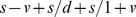
Figure 2. The 25 species avian phylogeny, representing 4 genera of birds from Maluridae family, estimated by QFM using the 227,700 embedded quartets in 18 gene trees.

The evolutionary relationships maintained by this tree are supported by the findings of the previous studies [38], [40], [41], [43].
Since we do not know the true trees for biological datasets, we have compared the result obtained from QFM with biological beliefs and other rigorous analyses. The tree returned by QFM (which is identical to the tree estimated by QMC) is quite interesting and consistent with the previous findings as discussed below.
• QFM has been able to correctly identify the clusters associated with the four genera of birds. Also, it has placed the group of Amytornis birds as the sister to the rest of the family, and the group of Stipiturus birds as the sister to Malurus and Clytomias birds. These evolutionary relationships maintained by QFM are supported by the findings of the previous studies [38], [40], [41].
• Amytornis: Using allozyme analysis, Christidis [41] has shown that A. barbatus is the earliest diverged lineage in the Amytornis genus. Same results have been obtained by a DNA sequencing study in [42]. The sequence-based analysis of Lee et al. [38] also have confirmed this. Our analyses with QFM also have found the same pattern. Lee et al. [38] also have shown that A. housei should be within the textilis complex, which is confirmed by our QFM tree.
• Stipiturus: Evolutionary relationships within the Stipiturus genus have been well studied [38], [40], [43]. Our study is consistent with the previous findings: S. mallee and S. ruficeps are closer to each other than they are to S. malachurus.
• Clytomyias and Malurus: C. insignis was placed to Stipiturus species by [40]. However, in a more recent extensive multi-locus study, Lee et al. [38] argued that C. insignis is closer to M. grayi. Our study has also confirmed this fact. Also our study has confirmed their [38] findings that M. alboscapulatus is closer to M. melanocephalus than to M. leucopterus.
Lee et al.
[38] showed that ILS is likely a general feature of the genetic history of these avian species. Since quartets are not prone to anomaly zone [19], [23], quartet based analyses to resolve the avian history is of high importance. Interestingly, both QMC and QFM resolved the evolutionary history of these  birds similarly. Therefore, we believe that this tree should be considered as a reasonable hypothesis about the evolutionary history of this family of birds.
Discussion
In this work we have presented a novel and highly accurate quartet amalgamation technique, which we refer to as QFM. We have demonstrated the superiority of our method over QMC, which is known to be the best quartet amalgamation method to date.
QFM is a new promising divide and conquer supertree method having an algorithmic appeal. We have conducted an extensive experimental study comparing QFM against QMC under different model conditions by varying different parameters. For almost all model conditions considered, QFM performs at least equal but in most cases better than QMC. In line with the experimental results shown in [9], we have found that quadratic sampling of quartets is not sufficient for accurate supertree construction. However, with  quartets, both QFM and QMC can reconstruct very accurate trees indicating that it is possible to reconstruct an accurate supertree from large number of quartets, even with high amount of noise in the input data. QFM has also been tested on real biological datasets and has been shown to perform pretty well. The tree estimated by QFM has maintained the important evolutionary relationships despite the presence of incomplete lineage sorting. This is particularly interesting because this suggests that we can use quartet-based technique to develop species tree estimation method (from multi-locus data), which is less susceptible to gene tree incongruence due to ILS.
Species tree estimation is frequently based on phylogenomic approaches that use multiple genes from throughout the genome. However, combining data on multiple genes is not a trivial task. Genes evolve through biological processes that include deep coalescence (also known as incomplete lineage sorting (ILS)), duplication and loss, horizontal gene transfer etc. As a result the individual gene histories can differ from each other [10]. Species tree estimation in the presence of ILS is a challenging task. Moreover, anomalous gene trees (AGTs) make this task even more complicated [19], [20]. It has been proven that AGTs cannot occur in quartets and thus the most probable quartets induced by the true gene trees represent the true species trees for the corresponding four species [19], [23], Therefore, quartets can be used to design statistically consistent methods (methods that have the statistical guarantee to construct the true species tree given sufficiently large number of true gene trees) for constructing the species tree from gene trees (which evolve with ILS) as follows. First, we compute the quartets induced by the gene trees. For every four species, there are three possible quartets. Given sufficiently large number of true gene trees, the most probable quartets (the most frequently occurring quartets) on every four species represent the true species trees for those four species. Thus combining the most probable quartets to get a single and coherent species tree is an statistically consistent approach for species tree estimation. In this context, we can formalize the maximum weighted quartet satisfiability problem as follows.
• Input: A set  of weighted quartets.
• Output: The species tree  such that
  maximizes the summation of the weights of the satisfied quartets in
  .
.
We can define the weight of a quartet  as the proportion of the gene trees that induce
  . We can also incorporate the branch lengths in defining the weights. One major advantage of QFM is that it can readily be adapted to take a set of weighted quartets as input without making any change in its algorithmic constructs. Therefore, we think QFM is an important contribution to the phylogenomic analyses, in particular for estimating species trees from a set of gene trees where gene trees can be discordant from each other due to ILS.
Another advantage of QFM lies in its flexibility in choosing the partition score function (see “Partition Score” section). QFM can be customized to take different scoring functions (i.e.,  ,
,  , etc.) without making any change in the algorithmic construct. We have observed that QFM may not give the same result for different scoring functions for the same dataset. So for different datasets, we may obtain better results by adapting different suitable scoring functions. Thus QFM provides us with the flexibility to change the scoring function as needed. In future we shall try to make our algorithm self-adaptable to the appropriate scoring function by analyzing different characteristics of the input datasets. Notably, as has already been discussed above, one shortcoming of the current implementation of QFM is that it is not as fast as QMC.
Materials and Methods
In this section we present our heuristic algorithm, namely, the Quartet FM (QFM) algorithm. Our algorithm employs a quartet based supertree reconstruction technique that involves a bipartition method inspired by the Fiduccia Mattheyses (FM) bipartition technique [32].
Basics
A quartet  is consistent with a tree
  if in
if in  , there is an edge (or path in general) separating
  and
and  from
from  and
and  . For any four taxa, only one quartet (out of
  possible quartets) will be consistent with a tree
  . In Figure 3 among the three quartets, quartet
  is consistent with tree
  as there exists an edge in
  such that it separates
  and
and  from
from  and
and  . Other two quartets are inconsistent with
  as no such edge exists in
  .
.
Figure 3. Quartet consistency with a tree  .
.

Among the three quartets, only  = ((
= (( ,
,  ), (
), ( ,
, )) is consistent with
  because
  has an internal edge that separates taxa
  and
and  from taxa
  and
and  in
in  .
.
A bipartition of an unrooted tree  is formed by taking any edge in
  , and writing down the two sets of taxa that would be formed by deleting that edge. Let
  be a tree over the taxa set
  . Now, if we take an internal edge
  of
of  and delete
  , then we get two subtrees, namely,
  and
and  . Let
. Let  and
and  be the sets of taxa of
  and
and  respectively. We shall denote such bipartition by (
 ,
,  ). Thus an internal edge in
  corresponds to a bipartition of
  .
.
A quartet  is satisfied with respect to a bipartition
  if taxa
  and
and  reside in one part and taxa
  and
and  reside in the other. A satisfied quartet is consistent with
  . The quartet
  is said to be violated with respect to a bipartition
  when taxa
  and
and  (or
(or  and
and  ) reside in one part and taxa
  and
and  (or
(or  and
and  ) reside in the other part. On the other hand,
  is said to be deferred with respect to a bipartition
  if any three of its four taxa reside in one part and the fourth one resides in the other.
A tree  over a taxa set
  is said to be a star, if
  has only one internal node and there is an edge from the internal node incident to each taxon
  . We shall refer to such a tree as a depth one tree.
Divide and conquer approach
We follow a divide and conquer approach similar to QMC [7]–[9]. Let,  be a set of quartets over a set of taxa,
  . We aim to construct a tree
  on
on  , satisfying the largest number of input quartets possible. The divide and conquer approach recursively creates bipartition of the taxa set, where each bipartition corresponds to an internal edge in the tree under construction. QMC uses a heuristic bipartition technique which is based on finding a maximum cut (MaxCut) in a graph over the taxa set, where the edges represent the input quartets [9]. On the other hand, our algorithm uses a heuristic bipartition algorithm inspired by the famous Fiduccia and Mattheyses (FM) [32] bipartition algorithm.
Divide
At each recursive step, we partition the taxa set  into two sets
  and
and  . We shall describe the bipartitioning algorithm in “Method of Bipartition” section. After the algorithm partitions the taxa set, it augments both parts (
 and
and  ) with a unique dummy (artificial) taxon. This taxon will play a role while returning from the recursion. After the addition of the dummy taxon to the sets
  and
and  , we subdivide the quartet set
  into two sets,
  and
and  . A quartet set
  takes those quartets
  from
from  such that either all four taxa
  ,
,  ,
,  and
and  or any three thereof belong to
  (here
(here  ). In other words, satisfied or violated quartets with respect to the partition
  are not considered to be included in either
  or
or  . Moreover, in every deferred quartet, where three taxa are in the same part, the other taxon is renamed by the name of the dummy taxon, and the quartet continues to the next step. Thus we get, two
  pairs:
  and
and  . We then recurse on both pairs
  and
and  if
if  is non-empty and

 . If either
  is empty or
  , we return a depth one tree over the taxa set
  .
.
Conquer
On returning from the recursion, at each step, we have two trees,  (corresponding to
  ) and
) and  (corresponding to
  ). These two trees are rerooted at the dummy taxon. Then the dummy taxon is removed from each tree and the two roots are joined by an internal edge.
Figure 4 describes the high level divide and conquer algorithm. Let  be the input quartet set and
  be the corresponding taxa set. Assume that
  =
=  ,
,  ,
,  ,
,  ,
,  ,
,  , and hence
  . First,
  is partitioned into two sets,
  and
and  by using the bipartition technique described in “Method of Bipartition” section. Here,
  is the dummy taxon. The bipartition
  satisfies quartets
  ,
,  and
and  from
from  . So these quartets will not be considered in the next level.
  takes
takes 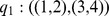 and
and 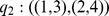 as three of the taxa of
  and
and  reside in
  . We replace the taxon which does not belong to
  with the dummy taxon
  . Hence we get
  . Similarly we get
 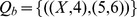 . Next we recurse on
  and
and  , and
, and  and
and  are partitioned further into
  and
and  , respectively. The partition
  satisfies
  and violates
  in
in  and
and  satisfies the only quartet in
  . So the quartet sets for the next level are empty and hence no more recursion is required. We return a depth one tree for each of the taxa sets
  ,
,  ,
,  and
and  . The returned trees are merged by removing the dummy taxon of that level and joining the branches of the dummy taxa. In Figure 4, the upper half shows the divide steps. The depth one trees are returned when no more recursion is required. The lower half of Figure 4 shows how the trees are returned and merged as the recursion unfolds (conquer step). Thus we get the final merged tree
 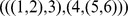 (shown at the bottom of Figure 4) satisfying
  quartets in total. The satisfied quartets are
  ,
,  ,
,  ,
,  and
and  .
.
Figure 4. Divide and conquer approach.

Divide: At each step, the input set of taxa of this step is partitioned into two sets and an unique dummy taxon is added to both sets. The input quartet set is then partitioned into two sets according to the bipartition of the set of taxa. So we get two (taxa set, quartet set) pairs, which are input to the successive divide steps. If at any step, the quartet set gets empty or the size of the taxa set becomes less than or equal to  , a depth one tree over the taxa set is returned. Conquer: At each step, there are two trees corresponding to the divide calls initiated at this step. These two trees are joined on the dummy taxon introduced at this step during divide. For example, the leftmost two depth one trees, when returned to its caller, are joined on the dummy taxon
  .
.
Method of Bipartition
The most crucial part of our algorithm is the bipartition (divide step) technique. Here, we differ from QMC [7]–[9] and adopt a new bipartition technique inspired by the famous Fiduccia and Mattheyses (FM) algorithm for bipartitioning a hyper graph minimizing the cut size [32]. In divide and conquer based phylogenetic tree construction, the bipartition of the taxa set corresponds to an internal edge of the tree under construction. An internal edge, in turn, plays a role to make quartets to be satisfied or violated against the bipartition. So we adopt a different bipartition technique from that used in QMC, with an objective to get better results.
Our bipartition algorithm takes a pair of taxa set and a quartet set ( ,
,  ) as input. It partitions
  into two sets, namely,
  and
and  with an objective that (
 ,
,  ) satisfies the maximum number of quartets from
  . The algorithm starts with an initial partition and iteratively searches for a better partition. We will use a heuristic search to find the best partition. Before we describe the steps of the algorithm, we describe the algorithmic components.
Partition Score
We assess the quality of a partition by assigning a partition score. We use a scoring function, 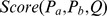 , such that the higher score will indicate a better partition. This function checks each
  against the partition
  and determines whether
  is satisfied, violated or deferred. We define the score function in terms of the number of satisfied and violated quartets. Let
  and
and  denote the number of satisfied and violated quartets. Then, two natural ways of defining the score function are: 1) taking the difference between the number of satisfied and violated quartets (
 ), and 2) taking the ratio of the number of satisfied and violated quartets (
 ). As num In this paper, we used
  as the score function. We can also use some other complicated score functions defined in terms of the number of satisfied, violated and deferred quartets (i.e.,
  , where
  denotes the number of deferred quartets). In our preliminary experimental study, we have explored different score functions and observed that
  gives better performance in most of the cases. Notably, although in some cases other functions (e.g.,
  ,
,  ) achieve better results than
  (results are not shown in this paper), none of them is consistently better than
  .
.
Gain Measure
Let  be a partition of set of taxa
  . Let
. Let  be a taxon and without loss of generality we assume that
  . Let
. Let  be the partition after moving the taxa
  from
from  to
to  . That means,
  , and
, and  . Then we define the gain of the transfer of the taxon
  with respect to
  , denoted by Gain
 , as
, as  .
.
Singleton Bipartition
A bipartition ( ) of
) of  is singleton if
  or
or  . In our bipartition algorithm, we keep a check for the singleton bipartition. We do not allow our bipartition algorithm to return a singleton bipartition to avoid the risk of an infinite loop.
Algorithm
Now we describe the bipartition algorithm which we call MFM (Modified FM) Bipartition Algorithm. Let, ( ,
,  ) be the input to the bipartition algorithm, where
  be a set of taxa and
  be a set of quartets over the taxa set
  . We start with an initial bipartition
  of
of  . The initial bipartitioning is done in four steps.
• Step 1: We count the frequency of each distinct quartet in  .
.
• Step 2: We then sort  by the frequency count of the quartets in a decreasing order.
• Step 3: Suppose after sorting 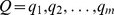 , where
  . Now we consider the quartets one by one in the sorted order. Initially both
  and
and  are empty.
Let 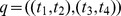 be a quartet in
  . If none of the
  taxa belongs to either
  or
or  , then we insert
  and
and  in
in  and
and  and
and  in
in  . Otherwise, if any of the
  taxa exists in either
  or
or  we take the following actions to insert a taxon which doest not exist in
  or
or  . We maintain an insertion order. We consider
  ,
,  ,
,  and
and  respectively.
– To insert  , we look for the partition of
  (if
(if  exists in any part) and insert
  into that partition. But if
  does not exist in either of the partitions, then we look for the partition of either
  or
or  (either of these two must exist in
  or
or  ) and insert
  into the other partition.
– To insert  , we look for the partition of
  and insert
  into that partition.
– To insert  , we look for the partition of
  (if
(if  exists in any part) and inset
  into that partition. But if
  does not exist in either of the partitions, then we look for the partition of either
  or
or  and insert
  into the other partition.
– To insert  , we look for the partition of
  and insert
  into that partition.
• Step 4: When we insert a taxon  to any part, we remove it from
  . After considering each
  and inserting taxa accordingly, if
  remains non-empty, we insert the remaining taxa to either part randomly.
Obtaining  , we search for a better partition iteratively. At each iteration, we perform a series of transfers of taxa from one partition set to the other to maximize the number of satisfied quartets. At the beginning of an iteration, we set the status of all the taxa as free. Then, for each free taxon
  , we calculate
  , and find the taxon
  with the maximum gain. There can be more than one taxa with the maximum gain where we need to break the tie. We will discuss this issue later. Next we transfer
  and set the status of this taxon as locked in the new partition that indicates that it will not be considered to be transferred again in this current iteration. This transfer creates the first intermediate bipartition
  . The algorithm then finds the next free taxon
  with the maximum gain with respect to
  , and transfer and lock that taxon to create another intermediate bipartition
  . Thus we transfer all the free taxon one by one. Let
  be the input quartet set and
  be the corresponding taxa set. Assume that
  =
=  ,
,  ,
,  ,
,  ,
,  ,
,  (same as used in Figure 4). Hence,
  . Following the steps of the initial bipartition, we get the initial bipartition
  and
and  . Figure 5 shows the first iteration of the bipartition algorithm for this particular example.
Figure 5. An example iteration of the Bipartition Algorithm MFM.

The locked taxa are shown in circles. At each step, the taxon which has the maximum gain and will be transferred from its current partition to the other is indicated by a left arrow. ( ,
,  ) is the initial bipartition of this iteration. Initially all taxa are free (i.e, not locked). The gain is computed for each free taxon of this step and the taxon (which is
  here) with maximum gain is transferred from its own partition to the other partition. Thus we get partition (
 ,
,  ), where
  is a locked taxon. In this way, only one taxon is locked at a step and once a taxon is locked, it remains locked throughout the iteration. An iteration completes when all taxa get locked. Here, all taxa get locked at (
 ,
,  ).
).
Suppose that the taxa are locked in the following order:  . That is,
  has been locked first, then
  ,
,  and so on. Let, the gain values of the corresponding partitions are:
Now we define the cumulative gain up to the  th transfer as
The maximum cumulative gain,  is defined as
In each iteration, the algorithm finds the current ordering ( ) of the transfers and saves this order in a log table along with the cumulative gains (see Table 3 for example). Let
  be the taxon in the log table corresponding to
  . This means that we obtain the maximum cumulative gain after moving the
  th taxon (with respect to the order stored in the log table). Then we rollback the transfers of the taxa (
 ) that were moved after
  . Let the resultant partition after these rollbacks is
  . This partition will be the initial partition for the next iteration. In this way, the algorithm continues as long as the maximum cumulative gain is greater than zero and returns the resultant bipartition. Table 3 lists the order of locking, corresponding gain and cumulative gain with respect to the iteration illustrated in Figure 5. From Table 3 we note that we get the maximum cumulative gain,
  , after moving taxon
  . Here, we also get the maximum value of cumulative gain after moving taxon
  . We break the tie arbitrarily. We consider the taxon for which we get the maximum cumulative gain for the first time. For this example, we get the maximum cumulative gain of
  at taxon
  for the first time. So we rollback all the subsequent moves. The resultant partition after this rollback is
  (partition
  in Figure 5). Similarly, Table 4 lists the ordering of locking, corresponding gain and cumulative gain with respect to the iteration which follows the iteration illustrated in Figure 5. From Table 4 we get that the maximum cumulative gain is
  . So the moves are rolled back and we get the final resultant partition
  .
.
Table 3. Gain Summary.

|

|

|

|

|

|

|

|

|

|

|

|

|

|

|

|

|

|

|

|

|

|

|

|

|

|

|

|
The log table corresponding to the iteration shown in Figure 5. Here  represents the step number. The input partition to step
  is (
is ( ,
,  ). The second column shows the taxon that has the maximum gain at the corresponding step, and the third column shows the corresponding maximum gain. The fourth column shows the cumulative gain of the gains listed in the third column. We observe that the cumulative gain gets maximum (
 ) after moving taxon
  in step
  . So all the subsequent moves of taxa are rolled back. The resultant partition of this iteration is (
 ,
,  ) =
) =  , which is the initial partition for the next iteration of the iteration in Figure 5.
Table 4. Gain Summary.

|

|

|

|

|

|

|

|

|

|

|

|

|

|

|

|

|

|

|

|

|

|

|

|

|

|

|

|
The log table corresponding to the next iteration of the iteration shown in Figure 5. Here  represents the step number. The input partition to step
  is (
is ( ,
,  ). The second column shows the taxon that has the maximum gain at the corresponding step, and the third column shows the corresponding maximum gain. We observe that the cumulative gain gets maximum (
 ) at step
  . So we rollback all the subsequent moves including the move at step
  and return the initial partition
  of this iteration as the resultant bipartition of the bipartition algorithm. No more iteration is needed as the maximum cumulative gain of the current iteration is not greater than zero.
As we have mentioned earlier, we do not allow any transfer of taxa that results into a singleton bipartition. Therefore, we need to add some additional conditions. Also, there could be more than one free taxa with the maximum gain, where we need to decide which one to transfer. We consider the following cases to address these issues. Let,  be a set of free taxa with the maximum gain.
• Case 1:  and at least one corresponding bipartition is not singleton. That means, there exists
  such that transfer of
  does not result into a singleton bipartition. Let
  be the set of taxa, that can be safely transferred without resulting in a singleton bipartition. Note that,
  . If
. If  , we transfer the taxa
  . Otherwise, we have more than one taxa in
  . In that case, we pick the taxon
  , for which the corresponding bipartition (after transferring
  ) satisfies maximum number of quartets (note that every taxa in
  has the same gain, but the corresponding bipartitions do not necessarily satisfy the same number of quartets). In the case of a tie, we choose one taxon at random.
• Case 2:  and transfer of each
  results in a singleton bipartition. In this case, we consider the set of taxa with the second highest maximum gain. Let
  be the set of free taxa with the second highest maximum gain. We then recursively check ‘Case 1’ and ‘Case 2’ on
  . If we cannot find a taxon that can be transferred without resulting into a singleton bipartition, we make the status of all the free taxa locked and set their gain to zero.
At each divide step we have a  pair as input. The bipartition algorithm returns a bipartition
  of the taxa set
  . We then divide
  into
into  and
and  and obtain
  and
and  pairs.
  and
and  will be further bipartitioned in subsequent divide steps. The pseudo-code of the bipartition method MFM is given in Table S4 in File S1. Moreover, the run time analyses of Algorithm MFM is described in .
Supporting Information
Supplementary material. Additional tables, and the pseudocode and time complexity of MFM bipartition algorithm are presented.
(PDF)
Acknowledgments
We thank Dr. Sagi Snir for appreciating our work, providing constructive suggestions and helping us with the QMC code and data.
Funding Statement
The authors have no support or funding to report. This work was done as a part of the master’s thesis work of Rezwana Reaz under the supervision of Dr. M. Sohel Rahman.
References
- 1.Linder CR, Warnow T (2005) An overview of phylogeny reconstruction. Handbook of Computational Molecular Biology.
- 2. Saitou N, Nei M (1987) The neighbor-joining method: A new method for reconstructing phylogenetic trees. Journal of Molecular Biology and Evolution 4: 406–425. [DOI] [PubMed] [Google Scholar]
- 3. Felsenstein J (1981) Evolutionary trees from dna sequences: a maximum likelihood approach. Journal of Molecular Evolution 17: 368–376. [DOI] [PubMed] [Google Scholar]
- 4. Fitch WM (1971) Toward defining the course of evolution: minimum change for a specific tree topology. Systematic Biology 20: 406–416. [Google Scholar]
- 5.Baum BR, Ragan MA (2004) The mrp method. In: Phylogenetic supertrees, Springer. pp. 17–34.
- 6. Regan MA (1992) Matrix representation in reconstructing phylogenetic relationships among the eukaryotes. Biosystems 28: 47–55. [DOI] [PubMed] [Google Scholar]
- 7. Snir S, Warnow T, Rao S (2008) Short quartet puzzling: A new quartet-based phylogeny reconstruction algorithm. Journal of Computational Biology 15: 91–103. [DOI] [PubMed] [Google Scholar]
- 8. Snir S, Rao S (2010) Quartets maxcut: A divide and conquer quartets algorithm. IEEE/ACM Transaction of Computational Biology and Bioinformatics 7: 704–718. [DOI] [PubMed] [Google Scholar]
- 9. Snir S, Rao S (2012) Quartet maxcut: A fast algorithm for amalgamating quartet trees. Journal of Molecular Phylogenetics and Evolution 62: 1–8. [DOI] [PubMed] [Google Scholar]
- 10. Maddison WP (1997) Gene trees in species trees. Systematic biology 46: 523–536. [Google Scholar]
- 11. Nichols R (2001) Gene trees and species trees are not the same. Trends in Ecology & Evolution 16: 358–364. [DOI] [PubMed] [Google Scholar]
- 12. Pamilo P, Nei M (1988) Relationships between gene trees and species trees. Molecular biology and evolution 5: 568–583. [DOI] [PubMed] [Google Scholar]
- 13. Tajima F (1983) Evolutionary relationship of dna sequences in finite populations. Genetics 105: 437–460. [DOI] [PMC free article] [PubMed] [Google Scholar]
- 14. Takahata N, Nei M (1985) Gene genealogy and variance of interpopulational nucleotide differences. Genetics 110: 325–344. [DOI] [PMC free article] [PubMed] [Google Scholar]
- 15.Kingman JF (1982) On the genealogy of large populations. Journal of Applied Probability: 27–43.
- 16. Rosenberg NA (2002) The probability of topological concordance of gene trees and species trees. Theoretical population biology 61: 225–247. [DOI] [PubMed] [Google Scholar]
- 17. Degnan JH, Salter LA (2005) Gene tree distributions under the coalescent process. Evolution 59: 24–37. [PubMed] [Google Scholar]
- 18.Harding E (1971) The probabilities of rooted tree-shapes generated by random bifurcation. Advances in Applied Probability: 44–77.
- 19. Degnan JH, Rosenberg NA (2006) Discordance of species trees with their most likely gene trees. PLoS genetics 2: e68. [DOI] [PMC free article] [PubMed] [Google Scholar]
- 20. Degnan JH, Rosenberg NA (2009) Gene tree discordance, phylogenetic inference and the multispecies coalescent. Trends in ecology & evolution 24: 332–340. [DOI] [PubMed] [Google Scholar]
- 21. Brown JK (1994) Probabilities of evolutionary trees. Systematic Biology 43: 78–91. [Google Scholar]
- 22. Steel M, McKenzie A (2001) Properties of phylogenetic trees generated by yule-type speciation models. Mathematical biosciences 170: 91–112. [DOI] [PubMed] [Google Scholar]
- 23. Degnan JH (2013) Anomalous unrooted gene trees. Systematic biology 62: 574–590. [DOI] [PubMed] [Google Scholar]
- 24. Larget BR, Kotha SK, Dewey CN, Ané C (2010) Bucky: Gene tree/species tree reconciliation with bayesian concordance analysis. Bioinformatics 26: 2910–2911. [DOI] [PubMed] [Google Scholar]
- 25. Allman ES, Degnan JH, Rhodes JA (2011) Identifying the rooted species tree from the distribution of unrooted gene trees under the coalescent. Journal of mathematical biology 62: 833–862. [DOI] [PubMed] [Google Scholar]
- 26. Strimmer K, von Haeseler A (1996) Quartet puzzling: A quartet maximum-likeihood method for reconstructing tree topologies. Journal of Molecular Biology and Evolution 13: 964–969. [Google Scholar]
- 27. Schmidt HA, Strimmer K, Vingron M, von Haeseler A (2002) Tree-puzzle: maximum likelihood phylogenetic analysis using quartets and parallel computing. Bioinformatics 18: 502–504. [DOI] [PubMed] [Google Scholar]
- 28. Strimmer K, Goldman N, von Haeseler A (1997) Bayesian probabilities and quartet puzzling. Journal of Molecular Biology and Evolution 14: 210–211. [Google Scholar]
- 29. Ranwez V, Gascuel O (2001) Quartet-based phylogenetic inference:improvement and limits. Journal of Molecular Biology and Evolution 18: 1103–1116. [DOI] [PubMed] [Google Scholar]
- 30.Xin L, Ma B, Zhang K (2007) A new quartet approach for reconstructing phylogenetic trees: Quartet joining method. Springer, LNCS 4598, pp. 40–50.
- 31. Swenson MS, Suri R, Linder CR, Warnow T (2011) An experimental study of quartets maxcut and other supertree methods. Algorithms for Molecular Biology 6: 7. [DOI] [PMC free article] [PubMed] [Google Scholar]
- 32.Fiduccia CM, Mattheyses RM (1982) A linear time heuristics for improving network partitions. Proc The 19th Design Automation Conference: 175–181.
- 33. Steel M (1992) The complexity of reconstructing trees from qualitative characters and subtrees. Journal of classification 9: 91–116. [Google Scholar]
- 34. Morgado A, Marques-Silva J (2010) Combinatorial optimization solutions for the maximum quartet consistency problem. Fundamenta Informaticae 102: 363–389. [Google Scholar]
- 35.Hodkinson TR, Parnell JA (2010) Reconstructing the tree of life: taxonomy and systematics of species rich taxa. CRC Press.
- 36. Robinson D, Foulds LR (1981) Comparison of phylogenetic trees. Mathematical Biosciences 53: 131–147. [Google Scholar]
- 37. Sanderson MJ, Donoghue MJ, Piel W, Eriksson T (1994) Treebase: a prototype database of phylogenetic analyses and an interactive tool for browsing the phylogeny of life. Amer Jour Bot 81: 183. [Google Scholar]
- 38.Lee JY, Joseph L, Edwards SV (2011) A species tree for the australo-papuan fairy-wrens and allies (aves: Maluridae). Systematic Biology. [DOI] [PubMed]
- 39. Zhaxybayeva O, Gogarten J, Charlebois R, Doolittle W, Papke R (2006) Phylogenetic analyses of cyanobacterial genomes: quantification of horizontal gene transfer events. Genome Research 16(9): 1099–1108. [DOI] [PMC free article] [PubMed] [Google Scholar]
- 40. Christidis L, Schodde R (1997) Relationships within the australo-papuan fairy-wrens (aves: Malurinae): an evaluation of the utility of allozyme data. Australian Journal of Zoology 45: 113–129. [Google Scholar]
- 41. Christidis L (1999) Evolution and biogeography of the australian grasswrens, amytornis (aves:Maluridae): biochemical perspectives. Australian journal of zoology 47: 113–124. [Google Scholar]
- 42. Christidis L, Rheindt FE, Boles WE, Norman JA (2010) Plumage patterns are good indicators of taxonomic diversity, but not of phylogenetic affinities, in australian grasswrens amytornis (aves:Maluridae). Molecular Phylogenetics and Evolution 57: 868–877. [DOI] [PubMed] [Google Scholar]
- 43. Donnellan SC, Armstrong J, Pickett M, Milne T, Baulderstone J, et al. (2009) Systematic and conservation implications of mitochondrial dna diversity in emu-wrens, stipiturus (aves: Maluridae). Emu 109: 143–152. [Google Scholar]
Associated Data
This section collects any data citations, data availability statements, or supplementary materials included in this article.
Supplementary Materials
Supplementary material. Additional tables, and the pseudocode and time complexity of MFM bipartition algorithm are presented.
(PDF)