Resampling-Based Empirical Bayes Multiple Testing Procedures for Controlling Generalized Tail Probability and Expected Value Error Rates: Focus on the False Discovery Rate and Simulation Study

Summary

This article proposes resampling-based empirical Bayes multiple testing procedures for controlling a broad class of Type I error rates, defined as generalized tail probability (gTP) error rates, gTP(q, g) = Pr(g(V_n, S_n) > q), and generalized expected value (gEV) error rates, gEV(g) = E[g(V_n, S_n)], for arbitrary functions g(V_n, S_n) of the numbers of false positives V_n and true positives S_n. Of particular interest are error rates based on the proportion g(V_n, S_n) = V_n/(V_n + S_n) of Type I errors among the rejected hypotheses, such as the false discovery rate (FDR), FDR = E[V_n/(V_n + S_n)]. The proposed procedures offer several advantages over existing methods. They provide Type I error control for general data generating distributions, with arbitrary dependence structures among variables. Gains in power are achieved by deriving rejection regions based on guessed sets of true null hypotheses and null test statistics randomly sampled from joint distributions that account for the dependence structure of the data. The Type I error and power properties of an FDR-controlling version of the resampling-based empirical Bayes approach are investigated and compared to those of widely-used FDR-controlling linear step-up procedures in a simulation study. The Type I error and power trade-off achieved by the empirical Bayes procedures under a variety of testing scenarios allows this approach to be competitive with or outperform the Storey and Tibshirani (2003) linear step-up procedure, as an alternative to the classical Benjamini and Hochberg (1995) procedure.

1 Introduction

1.1 Motivation and overview

Current statistical inference problems in areas such as astronomy, genomics, and marketing, routinely involve the simultaneous test of thousands, or even millions, of null hypotheses. These hypotheses concern a wide range of parameters, for high-dimensional multivariate distributions, with complex and unknown dependence structures among variables.

Type I error rates based on the proportion V_n/(V_n + S_n) of false positives among the rejected hypotheses (e.g., false discovery rate, FDR = E[V_n/(V_n + S_n)]) are especially appealing for large-scale testing problems, compared to traditional error rates based on the number V_n of false positives (e.g., family-wise error rate, FWER = Pr (V_n > 0)), as they do not increase exponentially with the number M of tested hypotheses.

However, only a handful of multiple testing procedures (MTP) are currently available for controlling such Type I error rates. Furthermore, existing methods suffer from a variety of limitations. Firstly, marginal procedures can lack power by failing to account for the dependence structure of the test statistics (Benjamini and Hochberg, 1995; Lehmann and Romano, 2005). Secondly, even for some of the marginal procedures, Type I error control relies on restrictive and hard to verify assumptions concerning the joint distribution of the test statistics, e.g., independence, dependence in finite blocks, ergodic dependence, positive regression dependence, and Simes’ Inequality (Benjamini and Hochberg, 1995, 2000; Benjamini and Yekutieli, 2001; Benjamini et al., 2006; Genovese and Wasserman, 2004b, a; Lehmann and Romano, 2005; Storey, 2002; Storey and Tibshirani, 2003; Storey et al., 2004). Thirdly, some procedures err conservatively by counting rejected hypotheses as Type I errors or estimating the proportion h₀/M of true null hypotheses by its upper bound of one (Benjamini and Hochberg, 1995; Dudoit and van der Laan, 2008; Dudoit et al., 2004a; van der Laan et al., 2004a).

Motivated by these observations, van der Laan et al. (2005) propose a resampling-based empirical Bayes procedure for controlling the tail probability for the proportion of false positives (TPPFP) among the rejected hypotheses, TPPFP(q) = Pr (V_n/(V_n + Sn) > q). The approach is extended in Dudoit and van der Laan (2008, Chapter 7) to control generalized tail probability (gTP) error rates, gTP (q, g) = Pr (g(V_n, S_n) > q), for arbitrary functions g(V_n, S_n) of the numbers of false positives V_n and true positives S_n. Dudoit and van der Laan (2008, Section 7.8) further remark that empirical Bayes procedures may be used to control generalized expected value (gEV) error rates, gEV(g) = E[g(V_n, S_n)], such as the false discovery rate, FDR = E[V_n/(V_n + S_n)], and other parameters of the distribution of functions g(V_n, S_n).

The two main ingredients in a resampling-based empirical Bayes procedure are the following distributions.

• A null distribution Q₀ (or estimator thereof, Q_0n) for M-vectors of null test statistics T_0n.

• A distribution $Q_0^{\mathcal{H}}$ (or estimator thereof, $Q_{0n}^{\mathcal{H}}$) for random guessed sets of true null hypotheses H_0n.

By randomly sampling null test statistics T_0n and guessed sets of true null hypotheses ${\mathcal{H}}_{0n}$, one obtains a distribution for a random variable representing the guessed g-specific function of the numbers of false positives and true positives (given the empirical distribution P_n), for any given rejection region. Rejection regions can then be chosen to control tail probabilities and expected values for this distribution at a user-supplied Type I error level α.

Our proposed empirical Bayes procedures seek to gain power by taking into account the joint distribution of the test statistics and by “guessing” the set ${\mathcal{H}}_0$ of true null hypotheses instead of conservatively setting ${\mathcal{H}}_0=\{1,\dots ,M\}$. In addition, unlike most MTPs controlling the proportion of false positives, they provide Type I error control for general data generating distributions, with arbitrary dependence structures among variables.

Note that the empirical Bayes approach outlined above is very general and modular, in the sense that it can be successfully applied to any distribution pair $(Q_{0n},Q_{0n}^{\mathcal{H}})$ that satisfies the assumptions of Dudoit and van der Laan (2008, Theorem 7.2). In particular, the common marginal non-parametric mixture model of Section 3.3 is only one among many reasonable candidate models for $Q_{0n}^{\mathcal{H}}$ that does not assume independence of the test statistics.

1.2 Outline

This article proposes resampling-based empirical Bayes multiple testing procedures for controlling a broad class of Type I error rates, defined as generalized tail probability error rates, gTP(q, g) = Pr (g(V_n, S_n) > q), and generalized expected value error rates, gEV(g) = E[g(V_n, S_n)], for arbitrary functions g(V_n, S_n) of the numbers of false positives V_n and true positives S_n.

The article is organized as follows. The remainder of this section provides a brief overview of the multiple hypothesis testing framework developed in Dudoit and van der Laan (2008). Section 2 focuses on the special case of the false discovery rate, FDR = E[V_n/(V_n + S_n)], and summarizes widely-used FDR-controlling linear step-up procedures (Benjamini and Hochberg, 1995, 2000; Benjamini et al., 2006; Storey, 2002; Storey and Tibshirani, 2003). Section 3 presents the resampling-based empirical Bayes multiple testing procedures proposed in Dudoit and van der Laan (2008, Chapter 7) and van der Laan et al. (2005) for controlling generalized tail probability and expected value error rates. In the simulation study of Sections 4 and 5, the Type I error and power properties of an FDR-controlling version of the resampling-based empirical Bayes approach are investigated and compared to those of FDR-controlling linear step-up procedures introduced in Section 2. Finally, Section 6 summarizes our findings and outlines ongoing work.

1.3 Multiple hypothesis testing framework

This section, based on Dudoit and van der Laan (2008, Chapter 1), introduces a general statistical framework for multiple hypothesis testing and discusses in turn the main ingredients of a multiple testing problem.

1.3.1 Null and alternative hypotheses

Consider a data generating distribution $P\in \mathcal{M}$, belonging to a model $\mathcal{M}$, i.e., a set of possibly non-parametric distributions.

Suppose one has a learning set ${\mathcal{X}}_n\equiv \{X_i:i=1,n\}\stackrel{\mathrm{IID}}{~}P$, of n independent and identically distributed (IID) random variables (RV) from P. Let P_n denote the empirical distribution of the learning set ${\mathcal{X}}_n$, which places probability 1/n on each X_i, i = 1,…, n.

Hypothesis testing is concerned with using observed data to make decisions regarding properties of, i.e., hypotheses for, the unknown distribution that generated these data.

Define $\mathcal{M}$ pairs of null and alternative hypotheses in terms of a collection of M submodels, $\mathcal{M}(m)\subseteq \mathcal{M}$, m = 1, …, M, for the data generating distribution P (Dudoit and van der Laan, 2008, Section 1.2.4). Specifically, the M null hypotheses and corresponding alternative hypotheses are defined, respectively, as

$$H_0(m)\equiv I(P\in \mathcal{M}(m))\text{and}{H}_1\text{(}m\text{)}\equiv I(P\notin \mathcal{M}(m)).$$ (1)

In many testing problems, the submodels concern parameters, i.e., functions $\mathrm{\Psi }(P)=\mathrm{\psi }=(\mathrm{\psi }(m):m=1,\dots ,M)\in {\mathbb{R}}^M$ of the data generating distribution P, and each null hypothesis H₀(m) refers to a single parameter, $\mathrm{\psi }(m)=\mathrm{\Psi }(P)(m)\in \mathbb{ℝ}$.

The complete null hypothesis $H_0^C$ states that the data generating distribution P belongs to the intersection ${{\displaystyle \cap }}_{m=1}^M\mathcal{M}(m)$ of the M submodels,

$$H_0^C\equiv {\displaystyle \prod _{m=1}^M{H}_0(m)=}{\displaystyle \prod _{m=1}^{M}I(P\in \mathcal{M}(m))}=I(P\in \underset{m=1}{\overset{M}{{\displaystyle \cap }}}\mathcal{M}(m)).$$ (2)

Let

$${\mathcal{H}}_0={\mathcal{H}}_0(P)\equiv \{m:H_0(m)=1\}=\{m:P\in \mathcal{M}(m)\}$$ (3)

denote the set of $h_0\equiv \left|{\mathcal{H}}_0\right|$ true null hypotheses, where the longer notation ${\mathcal{H}}_0(P)$ emphasizes the dependence of this set on the data generating distribution P. Likewise, let

$${\mathcal{H}}_1={\mathcal{H}}_1(P)\equiv \{m:H_1(m)=1\}=\{m:P\notin \mathcal{M}(m)\}={\mathcal{H}}_0^c(P)$$ (4)

be the set of $h_1\equiv \left|{\mathcal{H}}_1\right|=M-h_0$ false null hypotheses.

1.3.2 Test statistics

A testing procedure is a data-driven, i.e., random, rule for estimating the set of false null hypotheses ${\mathcal{H}}_1$, i.e., for deciding which null hypotheses should be rejected.

The decisions to reject or not the null hypotheses are based on an M-vector of test statistics, T_n = (T_n(m): m = 1, …, M), that are functions $T_n(m)=T(m,{\mathcal{X}}_n)=T(m;P_n)$ of the data ${\mathcal{X}}_n$, i.e., of the empirical distribution P_n (Dudoit and van der Laan, 2008, Section 1.2.5). Denote the typically unknown (finite sample) joint distribution of the test statistics T_n by Q_n = Qn(P).

Single-parameter null hypotheses of the form H₀(m) = I(ψ(m) ≤ ψ₀(m)) or I(ψ(m) = ψ₀(m)), m = 1,…, M, may be tested based on t-statistics (i.e., standardized differences),

$$T_n(m)\equiv \frac{\text{Estimator}-\text{Null value}}{\text{Standard error}}=\sqrt{n}\frac{{\mathrm{\psi }}_n(m)-{\mathrm{\psi }}_0(m)}{{\mathrm{\sigma }}_n(m)}.$$ (5)

Here, $\widehat{\mathrm{\Psi }}(P_n)={\mathrm{\psi }}_n=({\mathrm{\psi }}_n(m):m=1,\dots ,M)$ denotes an estimator of the parameter Ψ(P) = ψ = (ψ(m) : m = 1,…,M) and $({\mathrm{\sigma }}_n(m)/\sqrt{n}:m=1,\dots ,M)$ denotes the estimated standard errors for elements ψ_n(m) of ψ_n.

1.3.3 Multiple testing procedures

A multiple testing procedure (MTP) provides rejection regions C_n(m), i.e., sets of values for each test statistic T_n(m) that lead to the decision to reject the corresponding null hypothesis H₀(m) and declare that $P\notin \mathcal{M}(m)$, m = 1, …, M (Dudoit and van der Laan, 2008, Sections 1.2.6 and 1.2.7). In other words, a MTP produces a random (i.e., data-dependent) set of rejected null hypotheses ${\mathcal{R}}_n$ that estimates the set of false null hypotheses ${\mathcal{H}}_1$,

$${\mathcal{R}}_n=\mathcal{R}(T_n,Q_{0n},\mathrm{\alpha })\equiv \{m:T_n(m)\in {\mathcal{C}}_n(m)\}=\{m:H_0(m)\text{is rejected}\},$$ (6)

where ${\mathcal{C}}_n(m)=\mathcal{C}(m;T_n,Q_{0n},\mathrm{\alpha }),m=1,\dots ,M$, denote possibly random test statistic rejection regions.

We focus without loss of generality on one-sided rejection regions of the form ${\mathcal{C}}_n(m)=(c_n(m)+\infty )$, where $c_n=(c_n(m):m=1,\dots ,M)\in {\mathbb{ℝ}}^M$ is an M-vector of critical values or cut-offs.

1.3.4 Type I error rate and power

Errors in multiple hypothesis testing

In any testing problem, two types of errors can be committed (Dudoit and van der Laan, 2008, Section 1.2.8). A Type I error, or false positive, is committed by rejecting a true null hypothesis $({\mathcal{R}}_n\cap {\mathcal{H}}_0)$. A Type II error, or false negative, is committed by failing to reject a false null hypothesis $({\mathcal{R}}_n^C\cap {\mathcal{H}}_1)$.

Type I error rate

When testing multiple hypotheses, there are many possible definitions for the Type I error rate and power of a testing procedure. Accordingly, we define a Type I error rate as a parameter ${\mathrm{\theta }}_n=\mathrm{\Theta }(F_{V_n,R_n})$ of the joint distribution $F_{V_n,R_n}$ of the numbers of Type I errors $V_n=|{\mathcal{R}}_n\cap {\mathcal{H}}_0|$ and rejected hypotheses $R_n=\left|{\mathcal{R}}_n\right|$ (Dudoit and van der Laan, 2008, Section 1.2.9).

Such a representation covers a broad class of Type I error rates, defined as generalized tail probability (gTP) error rates,

$$\mathit{gTP}(q,g)\equiv \mathrm{Pr}(g(V_n,S_n)>q),$$ (7)

and generalized expected value (gEV) error rates,

$$\mathit{gEV}(g)\equiv E[g(V_n,S_n)],$$ (8)

for functions g(V_n; S_n) of the numbers of false positives V_n and true positives S_n = R_n − V_n.

Consider functions g that satisfy the following two natural monotonicity assumptions.

• Assumption MgV. The function g_s : υ → g(υ, s) is continuous and strictly increasing for any given s.

• Assumption MgS. The function g_υ : s → g(υ, s) is continuous and non-increasing for any given υ.

Of particular interest are the following two special cases, corresponding, respectively, to g-functions for the number and proportion of false positives among the rejected hypotheses. When g(υ, s) = υ, one recovers the generalized family-wise error rate (gFWER) and the per-family error rate (PFER). When g(υ, s) = υ/(υ + s), with the convention that υ/(υ + s) ≡ 0 if υ + s ≡ 0, one obtains the tail probability for the proportion of false positives (TPPFP) and the false discovery rate (FDR). Specifically, the FDR is defined as

$$\mathit{FDR}\equiv E\left[\frac{V_n}{\max \{R_n,1\}}\right]=E\left[\frac{V_n}{R_n}\right|V_n>0]\mathrm{Pr}(V_n>0)=E[\frac{V_n}{R_n}{R}_n>0]\mathrm{Pr}(R_n>0),$$ (9)

where R_n = V_n + S_n. Under the complete null hypothesis $H_0^C=I(P\in {{\displaystyle \cap }}_{m=1}^M\mathcal{M}(m))$, all R_n rejected hypotheses are Type I errors, hence V_n/R_n = 1 and FDR = FWER = Pr (V_n > 0).

Storey and Tibshirani (2003) and related articles (Storey, 2002; Storey et al., 2004) consider a variant of the FDR, termed the positive false discovery rate (pFDR),

$$\mathit{pFDR}\equiv E\left[\frac{V_n}{R_n}\right|R_n>0].$$ (10)

Note that FDR = pFDR × Pr (R_n > 0), so that, in general, FDR ≤ pFDR. An immediate flaw of the pFDR is that it is equal to one under the complete null hypothesis and therefore cannot be controlled under this testing scenario. By contrast, the FDR reduces to the family-wise error rate, FWER = Pr (V_n > 0).

Given the choice of a g-function representing the “cost” of Type I errors, there are a number of practical considerations that guide the decision to control the expected value vs. tail probabilities of this function (Dudoit and van der Laan, 2008, Section 3.5.1). By definition, gEV-controlling procedures only control g(V_n, S_n) on average and do not preclude large variations in this function. Furthermore, in some settings, one may wish to have high confidence (i.e., chance at least (1 − α)) that the cost function g(V_n;S_n) does not exceed an allowed bound q for false positives. In such cases, gTP control is a more appropriate form of Type I error control than gEV control. Finally, the parameter q confers flexibility to gTP-controlling MTPs and can be tuned to achieve a desired level of false positives.

The actual Type I error rate $\mathrm{\Theta }(F_{V_n,R_n})$ of a multiple testing procedure typically differs from its nominal Type I error level α, i.e., the level at which it claims to control Type I errors. Discrepancies between actual and nominal Type I error rates can be attributed to a number of factors, including the choice of a test statistics null distribution Q_0n and the type of rejection regions for a given choice of Q_0n. A testing procedure is said to be conservative if the nominal Type I error level a is greater than the actual Type I error rate, i.e., $\mathrm{\Theta }(F_{V_n,R_n})<\mathrm{\alpha }$, and anti-conservative if the nominal Type I error level a is less than the actual Type I error rate, i.e., $\mathrm{\Theta }(F_{V_n,R_n})<\mathrm{\alpha }$.

Power

Likewise, we define power as a parameter ${\mathrm{\vartheta }}_n=\mathrm{\Theta }(F_{U_n,R_n})$ of the joint distribution $F_{U_n,R_n}$ of the numbers of Type II errors $U_n=|{\mathcal{R}}_n^c\cap {\mathcal{H}}_1|$ and rejected hypotheses $R_n=\left|{\mathcal{R}}_n\right|$ (Dudoit and van der Laan, 2008, Section 1.2.10).

The average power, i.e., the expected value of the proportion of rejected hypotheses among the false null hypotheses, is defined as

$$\mathit{AvgPwr}\equiv \frac{1}{h_1}E[S_n]=1-\frac{1}{h_1}E[U_n].$$ (11)

1.3.5 Test statistics null distribution

One of the main tasks in specifying a multiple testing procedure is to derive rejection regions for the test statistics such that Type I errors are probabilistically controlled at a user-supplied level. However, one is immediately faced with the problem that the distribution of the test statistics is usually unknown.

In practice, the test statistics distribution Q_n = Qn(P) is replaced by a null distribution Q₀ (or estimator thereof, Q_0n) in order to derive rejection regions and resulting adjusted p-values. The choice of a proper null distribution is crucial in order to ensure that (finite sample or asymptotic) control of the Type I error rate under the assumed null distribution does indeed provide the desired control under the true distribution.

Dudoit and van der Laan (2008, Chapter 2) provide a general characterization for a proper test statistics null distribution, which leads to the explicit construction of two main types of test statistics null distributions.

The first original proposal of Dudoit et al. (2004b), van der Laan et al. (2004b), and Pollard and van der Laan (2004), defines the null distribution as the asymptotic distribution of a vector of null shift and scale-transformed test statistics, based on user-supplied upper bounds for the means and variances of the test statistics for the true null hypotheses (Dudoit and van der Laan, 2008, Section 2.3).

The second and most recent proposal of van der Laan and Hubbard (2006) defines the null distribution as the asymptotic distribution of a vector of null quantile-transformed test statistics, based on user-supplied test statistic marginal null distributions (Dudoit and van der Laan, 2008, Section 2.4).

For a broad class of testing problems, such as the test of single-parameter null hypotheses using t-statistics, a proper null distribution is the M-variate Gaussian distribution N(0, σ*), with mean vector zero and covariance matrix σ* = Σ* (P) equal to the correlation matrix of the vector influence curve for the estimator Ψ_n of the parameter of interest w (Dudoit and van der Laan, 2008, Section 2.6).

Resampling procedures (e.g., non-parametric or model-based bootstrap) are available to conveniently obtain consistent estimators of the null distribution and of the corresponding test statistic cut-offs, parameter confidence regions, and adjusted p-values (Dudoit and van der Laan, 2008, Procedures 2.3 and 2.4).

As detailed in Dudoit and van der Laan (2008, Section 2.8) and earlier articles, our multiple testing methodology differs in a number of fundamental aspects from existing approaches to Type I error control and the choice of a test statistics null distribution. In particular, we are only concerned with control of the Type I error rate under the true data generating distribution P. We are not concerned with strong control, i.e., with controlling the supremum of the Type I error rate over distributions that satisfy all 2^M possible subsets of null hypotheses. Indeed, as argued in Dudoit and van der Laan (2008, Section 2.8.1), the notions of weak and strong control of a Type I error rate become irrelevant in our framework. In addition, the definitions of weak and strong control are problematic as they implicitly assume the existence of a mapping ${\mathcal{J}}_0\to P_{{\mathcal{J}}_0}$, from subsets ${\mathcal{J}}_0\subseteq \{1,\dots ,M\}$ of null hypotheses to data generating distributions $P_{{\mathcal{J}}_0}\in {{\displaystyle \cap }}_{m\in {\mathcal{J}}_0}\mathcal{M}(m)$ that satisfy each of the null hypotheses in ${\mathcal{J}}_0$. Although strong control does consider the subset ${\mathcal{H}}_0={\mathcal{H}}_0(P)$ of true null hypotheses corresponding to the true data generating distribution P, Type I error control under P is not guaranteed by strong control, unless the mapping ${\mathcal{J}}_0\to P_{{\mathcal{J}}_0}$ results in $P_{{\mathcal{H}}_0}=P$. Strong control also involves restrictive assumptions such as subset pivotality. Note that the issue of strong control remains controversial and our position is at odds with commonly-accepted practice in the field of multiple testing.

1.3.6 Adjusted p-values

Adjusted p-values, for the test of multiple hypotheses, are defined as straightforward extensions of unadjusted p-values, for the test of single hypotheses (Dudoit and van der Laan, 2008, Section 1.2.12). Consider any multiple testing procedure ${\mathcal{R}}_n(\mathrm{\alpha })=\mathcal{R}(T_n,Q_{0n},\mathrm{\alpha })$, with rejection regions ${\mathcal{C}}_n(m;\mathrm{\alpha })=\mathcal{C}(m;T_n,Q_{0n},\mathrm{\alpha })$. One can define an M-vector of adjusted p-values, ${\tilde{\mathit{P}}}_{0n}=({\tilde{\mathit{P}}}_{0n}(m):m=1,\dots ,M)=\tilde{\mathit{P}}(T_n,Q_{0n})=\tilde{\mathit{P}}(T_n,Q_{0n},\mathrm{\alpha }):\mathrm{\alpha }\in [0,1])$, as

$$\begin{array}{l}{\tilde{\mathit{P}}}_{0n}(m)\equiv \inf \{\mathrm{\alpha }\in [0,1]:\text{Reject}{H}_0(m)\text{at nominal MTP level}\mathrm{\alpha }\}\\ =\inf \{\mathrm{\alpha }\in [0,1]:m\in {\mathcal{R}}_n(\mathrm{\alpha })\}\\ =\inf \{\mathrm{\alpha }\in [0,1]:T_n(m)\in {\mathcal{C}}_n(m;\mathrm{\alpha })\},m=1,\dots ,M.\end{array}$$ (12)

That is, the adjusted p-value ${\tilde{\mathit{P}}}_{0n}(m)$, for null hypothesis H₀(m), is the smallest nominal Type I error level (e.g., gFWER, TPPFP, or FDR) of the multiple hypothesis testing procedure at which one would reject H₀(m), given T_n.

As in single hypothesis tests, the smaller the adjusted p-value ${\tilde{\mathit{P}}}_{0n}(m)$, the stronger the evidence against the corresponding null hypothesis H₀(m). Thus, one rejects H₀(m) for small adjusted p-values ${\tilde{\mathit{P}}}_{0n}(m)$.

2 FDR-Controlling Linear Step-Up Multiple Testing Procedures

The following commonly-used FDR-controlling linear step-up procedures, such as Benjamini and Hochberg’s (1995) classical procedure and Storey and Tibshirani’s (2003) q-value procedure, require as their primary input an M-vector (P_0n(m) : m=1,…,M) of unadjusted p-values, computed under a test statistics null distribution Q₀ (or estimator thereof, Q_0n). The procedures are listed in Table 1.

Table 1. Simulation study: Multiple testing procedures.

This table summarizes the FDR-controlling procedures examined in the simulation study of Sections 4 and 5. The adaptive linear step-up procedures are based on generic Procedure 2.2, with specified estimators h_0n of the number of true null hypotheses h₀ (Sections 2 and 4.2.4). The resampling-based empirical Bayes procedures are based on Procedure 3.1, with specified estimators π_0n of the true null hypothesis prior probability π₀ (Sections 3 and 4.2.5).

LSU: Linear step-up procedures
	h0n
LSU.BH	M	Conservative: Benjamini and Hochberg (1995); Procedure 2.1
LSU.O	h0	Oracle
LSU.ABH	$h_{0n}^{\mathrm{ABH}}$	Adaptive: Benjamini and Hochberg (2000); Eq. (16)
LSU.TST	$h_{0n}^{\mathrm{TST}}(\mathrm{\alpha })$	Adaptive two-stage: Benjamini et al. (2006); Eq. (18), α = 0.05, 0.10
LSU.ST	$h_{0n}^{\mathrm{ST}}(\mathrm{\lambda })$	Adaptive: Storey and Tibshirani (2003); Procedure 2.3, Eq. (17)

EB: Resampling-based empirical Bayes procedures
	π0n
EB.C	1	Conservative
EB.O	h0/M	Oracle
EB.ABH	$h_{0n}^{\mathrm{ABH}}/M$	Adaptive: Benjamini and Hochberg (2000); Eq. (16)
EB.QV	$h_{0n}^{\mathrm{QV}}/M$	Adaptive q-value-based: Eq. (37)

2.1 Benjamini and Hochberg (1995) classical linear step-up procedure

In their seminal article, Benjamini and Hochberg (1995) propose the following FDR-controlling procedure.

Procedure 2.1 [FDR-controlling linear step-up Benjamini and Hochberg (1995) procedure]

Given an M-vector (P_0n(m) : m = 1,…, M) of unadjusted p-values, let O_n(m) denote the indices for the ordered unadjusted p-values, so that P_0n(O_n(1)) ≤ … < P_0n(O_n(M)). For controlling the FDR at nominal level α, the linear step-up procedure of Benjamini nand Hochberg (1995) yields the following set of rejected null hypotheses,

$${\mathcal{R}}_n(\mathrm{\alpha })=\{O_n(m):\exists h\ge \mathit{\text{m such that}}{P}_{0n}(O_n(h))\le \frac{h}{M}\mathrm{\alpha }\}.$$ (13)

That is, the mth most significant null hypothesis H₀(O_n(m)), with the m-th smallest unadjusted p-value P_0n(O_n(m)), is rejected if and only if it or at least one of the less significant null hypotheses H₀(O_n(h)), h ≥ m + 1, has an unadjusted p-value less than or equal to the corresponding cut-off αh/M. Adjusted p-values can be derived as

$${\tilde{\mathit{P}}}_{0n}(O_n(m))=\underset{h=m,\dots ,M}{\min }\left\{\min \right\{\frac{M}{h}{P}_{0n}(O_n(h)),1\left\}\right\},m=1,\dots ,M.$$ (14)

Note, however, that although Procedure 2.1 is a marginal procedure, proofs of FDR control rely on assumptions concerning the joint distribution of the test statistics. Benjamini and Hochberg (1995) prove that Procedure controls the FDR for independent test statistics. The subsequent article of Benjamini and Yekutieli (2001) establishes FDR control for test statistics with more general dependence structures, such as positive regression dependence.

2.2 Adaptive linear step-up procedures

Classical linear step-up Benjamini nand Hochberg (1995) Procedure 2.1 can be conservative, as Type I error control results show that it satisfies E[V_n/R_n] ≤ αh₀/M ≤ α, under certain assumptions on the joint distribution of the test statistics (e.g., independence, positive regression dependence). To remedy this conservativeness, Benjamini and colleagues have developed various adaptive procedures, involving the estimation of the number h₀ of true null hypotheses. Benjamini et al. (2006, Section 3) provide a nice review of such methods.

2.2.1 Generic adaptive linear step-up procedure

Procedure 2.2 [FDR-controlling generic adaptive linear step-up Benjamini et al. (2006, Definition 2) procedure]

Given an estimator h_0n of the number of true null hypotheses h₀, the generic adaptive linear step-up procedure of Benjamini et al. (2006, Definition 2) replaces the nominal Type I error level α in Benjamini and Hochberg (1995) Procedure 2.1 by the less conservative level of αM/h_0n > α.

Provided h_0n does not depend on the nominal Type I error level a, the adjusted p-values of an adaptive linear step-up procedure are simply the adjusted p-values of Procedure 2.1 scaled by M/h_0n,

$${\tilde{\mathit{P}}}_{0n}(O(m))=\frac{h_{0n}}{M}\underset{h=m,\dots ,M}{\min }\left\{\min \right\{\frac{M}{h}{P}_{0n}(O(h)),1\left\}\right\},m=1,\dots ,M.$$ (15)

Since h_0n/M ≤ 1, adaptive procedures lead to a larger number of rejected hypotheses than the standard Benjamini and Hochberg (1995) procedure (with h_0n/M = 1) applied with the same nominal FDR level α.

2.2.2 Benjamini and Hochberg (2000) adaptive linear step-up procedure

The adaptive linear step-up procedure of Benjamini and Hochberg (2000), summarized in Benjamini et al. (2006, Definition 3), derives the following estimator of the number of true null hypotheses based on graphical considerations.

$$h_{0n}^{\mathrm{ABH}}=\lceil \min \{h_{0n}(m_n),M\}\rceil ,$$ (16)

where

$$\begin{array}{l}{h}_{0n}(m)=\frac{M+1-m}{1-P_{0n}(O(m))},\\ m_n=\min \{m=2,\dots ,M:h_{0n}(m)>h_{0n}(m-1)\},\end{array}$$

and the ceiling ⌈x⌉ denotes the least integer greater than or equal to x, i.e., $\lceil x\rceil \in \mathbb{Z}$ and ⌈x⌉ − 1 < x ≤ ⌈x⌉.

Benjamini and Hochberg (2000) prove that this adaptive procedure controls the FDR for independent test statistics.

2.2.3 Storey and Tibshirani (2003) adaptive linear step-up procedure

Benjamini et al. (2006, Definition 5) show that the so-called q-value procedure of Storey (2002) and Storey and Tibshirani (2003), further discussed in Section 2.3, below, is a particular type of adaptive linear step-up procedure, with estimated number of true null hypotheses defined as

$$h_{0n}^{\mathrm{ST}}(\mathrm{\lambda })=\frac{\left|\right\{m:P_{0n}(m)>\mathrm{\lambda }\left\}\right|}{1-\mathrm{\lambda }},$$ (17)

in terms of a to-be-determined tuning parameter λ ∈ [0, 1], as in Procedure 2.3 in the expanded version of the article.

2.2.4 Benjamini et al. (2006) adaptive two-stage linear step-up procedure

Benjamini et al. (2006, Section 4, Definition 6) propose an adaptive two-stage linear step-up procedure (TST), whereby the estimator of the number of true null hypotheses h₀ is obtained from a one-stage application of standard linear step-up Benjamini and Hochberg (1995) Procedure 2.1. Specifically, the estimator of h₀ is defined in terms of the number $R_n^1(\mathrm{\alpha }/(1+\mathrm{\alpha }))$ of rejected hypotheses from a one-stage application of Procedure 2.1 with nominal FDR level α(1 + α),

$$h_{0n}^{\mathrm{TST}}(\mathrm{\alpha })=(1+\mathrm{\alpha })(M-R_n^1(\mathrm{\alpha }(1+\mathrm{\alpha }))).$$ (18)

Benjamini et al. (2006, Section 5) prove that the TST procedure controls the FDR for independent test statistics.

A multi-stage extension of Procedure 2.1 is also proposed (Benjamini et al., 2006, Definition 7).

Note that the estimated number of true null hypotheses $h_{0n}^{\mathrm{TST}}(\mathrm{\alpha })$ depends on the nominal Type I error level a. As a result, one cannot obtain closed form expressions (e.g., as in Eq. (15)) for the adjusted p-values of the two-stage procedure.

A practical question of interest is the nature and strength of the dependence of the estimated number of true null hypotheses $h_{0n}^{\mathrm{TST}}(\mathrm{\alpha })$ on the nominal Type I error level a. In general, $h_{0n}^{\mathrm{TST}}(\mathrm{\alpha })$ is not monotonic in α, as $M-R_n^1(\mathrm{\alpha }/(1+\mathrm{\alpha }))$ decreases with a, while 1 + α increases with α. Extreme cases are $h_{0n}^{\mathrm{TST}}(0)=M$ and $h_{0n}^{\mathrm{TST}}(1)=2(M-R_n^1(1/2))$.

2.3 Storey and Tibshirani (2003) adaptive linear step-up procedure

Please refer to the website companion for a complete discussion of the Storey and Tibshirani (2003) adaptive linear step-up procedure.

3 Resampling-Based Empirical Bayes Multiple Testing

This section presents the resampling-based empirical Bayes multiple testing approach proposed in Dudoit and van der Laan (2008, Chapter 7) and van der Laan et al. (2005), for controlling generalized tail probability and expected value error rates. The interested reader is referred to these earlier publications for further detail, including a proof of Type I error control, the derivation of adjusted p-values, and connections to the frequentist FDR-controlling linear step-up procedure of Benjamini and Hochberg (1995).

3.1 Resampling-based empirical Bayes multiple testing procedure

Given random M-vectors of test statistics Z₀ = (Z₀(m) : m = 1,…, M) and Z = (Z(m) : m = 1,…, M), a set of null hypotheses $\mathcal{H}\subseteq \{1,\dots ,M\}$, and an M-vector of cut-offs $c=(c(m):m=1,\dots ,M)\in {\mathbb{ℝ}}^M$ that define one-sided rejection regions of the form $\mathcal{C}(m)=(c(m),+\infty )$, introduce the following notation for the number of false positives (i.e., Type I errors), the number of true positives, the number of rejected hypotheses, and a function g of the numbers of false positives and true positives,

$$\begin{array}{c}V(c;\mathcal{H},Z)\equiv {\displaystyle \sum _{m\in \mathcal{H}}I(Z(m)>c(m)),}\\ S(c;\mathcal{H},Z)\equiv {\displaystyle \sum _{m\notin \mathcal{H}}I(Z(m)>c(m)),}\\ R(c;\mathcal{H},Z_0,Z)\equiv V(c;\mathcal{H},Z_0)+S(c;\mathcal{H},Z),\end{array}$$ (19)

and

$$G(c;\mathcal{H},Z_0,Z)\equiv g(V(c;\mathcal{H},Z_0),S(c;\mathcal{H},Z)).$$

In addition, define the following g-specific function for the generalized tail probability gTP(q; g) = Pr (g(V_n; S_n) > q) and expected value gEV(g) = E[g(V_n; S_n)] error rates,

$$\tilde{G}(c;\mathcal{H},Z_0,Z)\equiv \{\begin{array}{lll}I(G(c;\mathcal{H},Z_0,Z)>q)\hfill & \text{for}\hfill & \mathit{gTP}(q,g)\hfill \\ G(c;\mathcal{H},Z_0,Z)\hfill & \text{for}\hfill & \mathit{gTP}(g),\hfill \end{array}$$ (20)

so that these error rates can be expressed as

$${\mathrm{\theta }}_n(c)\equiv E[\tilde{G}(c;{\mathcal{H}}_0,T_n,T_n)].$$ (21)

In order to control gTP(q; g) and gEV(g) at level α, one seeks cut-offs c_n = (c_n(m) : m = 1,…,M), for the test statistics T_n = (T_n(m) : m = 1,…,M) ~ Q_n, so that the following Type I error constraint is satisfied,

$$\begin{array}{l}{\mathrm{\theta }}_n(c_n)=E[\tilde{G}(c_n;{\mathcal{H}}_0,T_n,T_n)]\le \mathrm{\alpha }[\text{finite sample control}]\\ \underset{n\to \infty }{\text{lim sup}}{\mathrm{\theta }}_n(c_n)=\underset{n\to \infty }{\text{lim sup}}E[\tilde{G}(c_n;{\mathcal{H}}_0,T_n,T_n)])\le \mathrm{\alpha }[\text{asymptotic control}].\end{array}$$ (22)

However, one is immediately faced with the problem that the distribution of $G(c_n;{\mathcal{H}}_0,T_n,T_n)$ depends on the unknown data generating distribution P, via the unknown set of true null hypotheses ${\mathcal{H}}_0$ and joint distribution Q_n of the test statistics T_n.

The resampling-based empirical Bayes approach replaces the unknown g-specific function of the numbers of false positives and true positives $G(c_n;{\mathcal{H}}_0,T_n,T_n)$ by the corresponding guessed function $G(c_n;{\mathcal{H}}_{0n},T_{0n},T_n)$, where T_n ~ Q_n is the M-vector of observed test statistics, T_0n ~ Q_0n is an M-vector of null test statistics, and ${\mathcal{H}}_{0n}~Q_{0n}^{\mathcal{H}}$ is a guessed set of true null hypotheses.

The null test statistics T_0n and the guessed sets H_0n are sampled independently, given the empirical distribution P_n, from distributions Q_0n and $Q_{0n}^{\mathcal{H}}$, chosen conservatively so that the guessed function $G(c_n;{\mathcal{H}}_{0n},T_{0n},T_n)$ is asymptotically stochastically greater than the corresponding true function $G(c_n;{\mathcal{H}}_0,T_n,T_n)$.

Procedure 3.1 [gTP- and gEV-controlling resampling-based empirical Bayes procedure]

Consider the simultaneous test of M null hypotheses H₀(m), m = 1, …, M, based on an M-vector of test statistics T_n = (T_n(m) : m = 1, …, M), with distribution Q_n = Q_n(P). Given a function g, that satisfies monotonicity Assumptions MgV and MgS, the following resampling-based empirical Bayes procedure may be used to control the generalized tail probability error rate, gTP(q; g) = Pr (g(V_n;S_n) > q), and the generalized expected value error rate, gEV(g) = E[g(V_n; S_n)].

1. Generate B pairs $\{(T_{0n}^b,{\mathcal{H}}_{0n}^b):b=1,\dots ,B\}$ of null test statistics $T_{0n}^b$ and random guessed sets ${\mathcal{H}}_{0n}^b$ of true null hypotheses as follows.

   1. The M-vectors of null test statistics $T_{0n}^b$ have a null distribution Q_0n, such as the bootstrap-based null-transformed test statistics null distributions described in Section 3.2 and Dudoit and van der Laan (2008, Chapter 2).
   2. The random guessed sets of true null hypotheses ${\mathcal{H}}_{0n}^b$ have a distribution $Q_{0n}^{\mathcal{H}}$ that corresponds to M independent Bernoulli random variables with parameters π_0n(T_n(m)). That is, generate binary random M-vectors $H_{0n}^b=(H_{0n}^b(m):m=1,\dots ,M)$ of null hypotheses as

      $$H_{0n}^b(m)\stackrel{\perp }{~}\text{Bernoulli}({\mathrm{\pi }}_{0n}(T_n(m))),m=1,\dots ,M,$$ (23)

      and define sets

      $${\mathcal{H}}_{0n}^b\equiv \{m:{\mathcal{H}}_{0n}^b(m)=1\}.$$ (24)

      Here, π_0n(t) is an estimated true null hypothesis posterior probability function, such as the estimated local q-value function

      $${\mathrm{\pi }}_{0n}(t)=\min \{1,\frac{{\mathrm{\pi }}_{0n}{f}_{0n}(t)}{f_n(t)}\},$$ (25)

      corresponding to the marginal non-parametric mixture model of Section 3.3.
   3. Null test statistics $T_{0n}^b$ and guessed sets ${\mathcal{H}}_{0n}^b$ are independent, given the empirical distribution P_n.
2. For any given test statistic cut-off vector c = (c(m) : m = 1,…, M), compute, for each of the B pairs $(T_{0n}^b,{\mathcal{H}}_{0n}^b)$, the corresponding guessed g-specific function of the numbers of false positives and true positives,

   $$G(c;{\mathcal{H}}_{0n}^b,T_{0n}^b,T_n)=g(V(c;{\mathcal{H}}_{0n}^b,T_{0n}^b),S(c;{\mathcal{H}}_{0n}^b,T_n)).$$ (26)

   An estimator of the (gTP or gEV) Type I error rate ${\mathrm{\theta }}_n(c)=E[\tilde{G}(c;{\mathcal{H}}_0,T_n,T_n)]$ is then given by

   $${\widehat{\mathrm{\theta }}}_n(c)=\frac{1}{B}{\displaystyle \sum }_{b=1}^B\tilde{G}(c;{\mathcal{H}}_{0n}^b,T_{0n}^b,T_n).$$ (27)
3. For user-supplied Type I error level α ∈ (0, 1), derive a cut-off vector c_n that satisfies the empirical Type I error constraint

   $${\widehat{\mathrm{\theta }}}_n(c_n)\le \mathrm{\alpha }.$$ (28)
   Common-cut-off procedure. The common cut-off γ_n is the smallest (i.e., least conservative) value g for which the constraint in Eq. (28) is satisfied. That is,

   $${\mathrm{\gamma }}_n\equiv \inf \{\mathrm{\gamma }\in \mathbb{ℝ}:{\widehat{\mathrm{\theta }}}_n({\mathrm{\gamma }}^{(M)})\le \mathrm{\alpha }\},$$ (29)

   where γ^(M) denotes the M-vector with all elements equal to γ, i.e., γ^(M) (m)= γ, ∀m = 1,…, M. The adjusted p-values may be approximated as

   $${\tilde{p}}_{0n}(o_n(m))\underset{¯}{\approx }\underset{h\in {\mathcal{O}}_n(m)}{\min }{\widehat{\mathrm{\theta }}}_n({(t_n(h))}^{(M)}),$$ (30)

   where O_n(m) denote the indices for the ordered test statistics T_n(O_n(m)), so that T_n(O_n(1)) ≥ … ≥ T_n(O_n(M)), and ${\overline{\mathcal{O}}}_n(m)\equiv \{O_n(m),\dots ,O_n(M)\}$.
   Common-quantile procedure. The common quantile probability δ_n, corresponding to the test statistics null distribution Q_0n, is the smallest (i.e., least conservative) value δ for which the constraint in Eq. (28) is satisfied. That is,

   $${\mathrm{\delta }}_n\equiv \inf \{\mathrm{\delta }\in [0,1]:{\widehat{\mathrm{\theta }}}_n(q_{0n}^{-1}(\mathrm{\delta }))\le \mathrm{\alpha }\},$$ (31)

   where $q_{0n}^{-1}(\mathrm{\delta })=(Q_{0n,m}^{-1}(\mathrm{\delta }):m=1,\dots ,M)$ denotes the M-vector of δ-quantiles for the null distribution Q_0n.
   The adjusted p-values may be approximated as

   $${\tilde{p}}_{0n}(o_n(m))\underset{¯}{\approx }\underset{h\in {\overline{\mathcal{O}}}_n(m)}{\min }\widehat{\mathrm{\theta }}(q_{0n}^{-1}(1-p_{0n}(h))),$$ (32)

   where p_0n(m) = 1 − Q_0n;m(t_n(m)) is the unadjusted p-value for null hypothesis H₀(m), O_n(m) denote the indices for the ordered unadjusted p-values P_0n(O_n(m)), so that P_0n(O_n(1)) ≤ … ≤ P_0n(O_n(M)), and ${\overline{\mathcal{O}}}_n(m)\equiv \{O_n(m),\dots ,O_n(M)\}$.

The proof for gEV control (and, in particular, FDR control) is an adaptation of the proof provided in Dudoit and van der Laan (2008, Theorem 7.2) for gTP control.

The two main ingredients of a resampling-based empirical Bayes procedure are discussed next: the null distribution Q₀ (or estimator thereof, Q_0n) for the M-vectors of null test statistics T_0n (Section 3.2) and the distribution $Q_0^{\mathcal{H}}$ (or estimator thereof, $Q_{0n}^H$) for the random guessed sets of true null hypotheses ${\mathcal{H}}_{0n}$ (Section 3.3). Further detail can be found in Dudoit and van der Laan (2008, Chapter 7) and van der Laan et al. (2005).

3.2 Distribution for the null test statistics

Test statistics null distributions are briefly discussed in Sections 1.3.5 and 4.2.3 of the present article and in depth in Dudoit and van der Laan (2008, Chapters 2 and 7).

3.3 Distribution for the guessed sets of true null hypotheses

This section presents only one among many reasonable approaches for specifying a distribution $Q_{0n}^H$ for the guessed sets of true null hypotheses, that does not assume independence of the test statistics.

3.3.1 Common marginal non-parametric mixture model

Consider M identically distributed pairs of test statistics and null hypotheses ((T_n(m); H₀(m)) : m = 1,…,M). Test statistics are assumed to have the following common marginal non-parametric mixture distribution,

$$T_n(m)~f\equiv {\mathrm{\pi }}_0{f}_0+(1-{\mathrm{\pi }}_0)f_1,m=1,\dots ,M,$$ (33)

where π₀ denotes the prior probability of a true null hypothesis, f₀ the marginal null density of the test statistics, and f₁ the marginal alternative density of the test statistics, i.e., π₀ ≡ Pr (H₀(m) = 1), T_n(m)|{H₀(m) = 1} ~ f₀, and T_n(m)|{H₀(m) = 0} ~ f₁.

3.3.2 Local q-values

A parameter of interest, for generating guessed sets of true null hypotheses under the marginal non-parametric mixture model of Eq. (33), is the local q-value function, i.e., the posterior probability function for a true null hypothesis H₀(m), given the corresponding test statistic T_n(m),

$${\mathrm{\pi }}_0(t)\equiv \mathrm{Pr}(H_0(m)=1|T_n(m)=t)=\frac{{\mathrm{\pi }}_0{f}_0(t)}{f(t)},m=1,\dots ,M.$$ (34)

Empirical Bayes q-values are similar in some sense to frequentist p-values: the smaller the q-value π₀(T_n(m)), the stronger the evidence against the corresponding null hypothesis H₀(m).

In practice, the local q-value function π₀(t) is unknown, as it depends on the unknown true null hypothesis prior probability π₀, test statistic marginal null density f₀, and test statistic marginal density f. Estimators of π₀(t) may be obtained by the plug-in method, from estimators of the three main parameters, π₀, f₀, and f, of the mixture model of Eq. (33).

Note that the q-values defined here in Eq. (34) are different in nature from the q-values of the linear step-up procedure of Storey and Tibshirani (2003), as the latter are actually adjusted p-values for FDR control (Eqs. (20) and (29), expanded version of the article).

3.3.3 Estimation of the true null hypothesis prior probability π₀

A trivial estimator π_0n of the prior probability π₀ of a true null hypothesis is the conservative value of one, i.e., π_0n = 1.

Alternately, π₀ may be estimated from prior knowledge or as a by-product of a computationally convenient procedure, such as the FDR-controlling adaptive linear step-up procedure of Benjamini and Hochberg (2000) or two-stage linear step-up procedure of Benjamini et al. (2006).

Various approaches are summarized in Table 1 and Section 4.2.5.

3.3.4 Estimation of the test statistic marginal null density f₀

For the test of single-parameter null hypotheses using t-statistics, the common marginal null density f₀ is simply a standard Gaussian density, i.e., T_n(m) | {H₀(m) = 1g ~ N(0, 1) (Section 4.2.5).

For other types of test statistics, one may estimate f₀ by kernel density smoothing of the M × B pooled elements of a matrix ${\mathit{Z}}_n^B$ of null-transformed bootstrap test statistics (Dudoit and van der Laan, 2008, Procedures 2.3 and 2.4).

3.3.5 Estimation of the test statistic marginal density f

For the test of single-parameter null hypotheses using t-statistics, the common marginal density f may be estimated based on an estimator of the asymptotic M-variate Gaussian distribution of the M-vector of t-statistics T_n (Section 4.2.5).

For other types of test statistics, one may estimate f by kernel density smoothing of the M × B pooled elements of a matrix ${\mathit{T}}_n^B$ of raw (before null transformation) bootstrap test statistics (Dudoit and van der Laan, 2008, Procedures 2.3 and 2.4).

3.4 Estimation of the proportion of true null hypotheses

A parameter of interest in multiple hypothesis testing is the number of true null hypotheses h₀. The following two estimators of h₀ may be obtained as by-products of the resampling-based empirical Bayes approach.

3.4.1 q-value-based empirical Bayes estimator

In the Bayesian context of Section 3.3, the local q-value function π₀(t), used to generate the random guessed sets of true null hypotheses in Procedure 3.1, is a posterior probability function for the true null hypotheses (Eq. (34)).

The prior probability π₀ = Pr (H₀(m) = 1) of a true null hypothesis yields an a priori, i.e., non data-driven, estimator of the number h₀ of true null hypotheses. Indeed, the a priori expected value of h₀ is

$$E[h_0]=E[{\displaystyle \sum }_{m=1}^{M}I(H_0(m)=1)]={\displaystyle \sum }_{m=1}^M\mathrm{Pr}(H_0(m)=1)=M{\mathrm{\pi }}_0.$$ (35)

The local q-values π₀(T_n (m)) = Pr (H₀(m) = 1| T_n(m)) are posterior probabilities for the true null hypotheses and in turn lead to the following a posteriori, i.e., data-driven, estimator of h₀. The a posteriori expected value of h₀ is

$$\begin{array}{l}E[h_0|{\mathcal{X}}_n]=E[{\displaystyle \sum _{m=1}^{M}I(H_0(m)=1)|{\mathcal{X}}_n}]\\ ={\displaystyle \sum _{m=1}^M\mathrm{Pr}(H_0(m)=1|{\mathcal{X}}_n)}\\ ={\displaystyle \sum _{m=1}^M\mathrm{Pr}(H_0(m)=1|T_n(m))}\\ ={\displaystyle \sum _{m=1}^M{\mathrm{\pi }}_0(T_n(m)),}\end{array}$$ (36)

under the assumption that the null hypotheses H₀(m) are conditionally independent of the data ${\mathcal{X}}_n$ given the corresponding test statistics T_n(m).

Thus, the number of true null hypotheses h₀ may be estimated by the sum of the estimated local q-values,

$$h_{0n}^{\mathrm{QV}}={\displaystyle \sum _{m=1}^M{\mathrm{\pi }}_{0n}(T_n(m))}.$$ (37)

3.4.2 Resampling-based empirical Bayes estimator

A resampling-based empirical Bayes estimator of the number of true null hypotheses h₀ can also be obtained as a by-product of Procedure 3.1, by averaging the cardinality $\left|{\mathcal{H}}_{0n}^b\right|$ of the guessed sets of true null hypotheses,

$$h_{0n}^{\mathrm{REB}}=\frac{1}{B}{\displaystyle \sum _{b=1}^B|{\mathcal{H}}_{0n}^b|}.$$ (38)

Keeping track of the B guessed numbers $\left|{\mathcal{H}}_{0n}^b\right|$ of true null hypotheses provides some indication of the stability of the guessed sets.

The above two estimators should be very similar. Indeed, the q-value-based estimator $h_{0n}^{\mathrm{QV}}$ is the expected value of the guessed numbers $\left|{\mathcal{H}}_{0n}^b\right|$ of true null hypotheses and, for a large number B of resampled datasets, the empirical mean $h_{0n}^{\mathrm{REB}}$ should converge to its expected value of $h_{0n}^{\mathrm{QV}}$.

4 Simulation Study

4.1 Simulation model

Simulated data consist of learning sets ${\mathcal{X}}_n=\{X_i:i=1,\dots ,n\}\stackrel{\mathrm{IID}}{~}N(\mathrm{\psi },\mathrm{\sigma })$, of n independent and identically distributed random variables from an M-variate Gaussian data generating distribution P, with mean vector Ψ = (Ψ(m) : m = 1,…,M) = Ψ(P) = E[X] and covariance matrix σ = (σ(m, m′) : m, m′ = 1,…, M) = Σ(P) = Cov [X]. The shorter notation σ²(m) ≡ σ(m, m) may be used for variances and the correlation matrix corresponding to σ is denoted by σ* = Σ* (P) = Cor [X].

Both the mean vector Ψ and the covariance matrix σ are treated as unknown parameters; the parameter of interest is the mean vector Ψ.

4.2 Multiple testing procedures

4.2.1 Null and alternative hypotheses

The simulation study concerns the two-sided test of the M null hypotheses H₀(m) = I(Ψ(m) = Ψ₀(m)) vs. the alternative hypotheses H1(m) = I(Ψ(m) ≠ Ψ₀(m)), m = 1,…, M. For simplicity, and without loss of generality, the null values are set equal to zero, i.e., Ψ₀(m) = 0.

4.2.2 Test statistics

The M null hypotheses are tested based on usual one-sample t-statistics,

$$T_n(m)\equiv \sqrt{n}\frac{{\mathrm{\psi }}_n(m)-{\mathrm{\psi }}_0(m)}{{\mathrm{\sigma }}_n(m)},$$ (39)

where ${\mathrm{\psi }}_n(m)={\overline{X}}_n(m)={{\displaystyle \sum }}_i{X}_i(m)/n$ and ${\mathrm{\sigma }}_n^2(m)={{\displaystyle \sum }}_i{(X_i(m)-{\overline{X}}_n(m))}^2/(n-1)$ denote, respectively, the empirical means and variances for the M elements of X.

4.2.3 Test statistics null distribution

The unknown asymptotic joint null distribution Q₀ of the t-statistics of Eq. (39) is the M-variate Gaussian distribution N(0, σ*), with mean vector zero and covariance matrix equal to the unknown correlation matrix σ* of X.

A parametric estimator Q_0n of Q₀ is the Gaussian distribution $N(0,{\mathrm{\sigma }}_n^{\ast })$, where ${\mathrm{\sigma }}_n^{\ast }$ is the empirical correlation matrix of the learning set X_n.

This joint distribution Q_0n can be approximated by the empirical distribution of the B columns $\{Z_n^B(\cdot ,b)~N(0,{\mathrm{\sigma }}_n^{\ast }):b=1,\dots ,B\}$ of a matrix $Z_n^B$ simulated from $N(0,{\mathrm{\sigma }}_n^{\ast })$.

4.2.4 FDR-controlling linear step-up procedures

The simulation study examines the following five linear step-up procedures, summarized in Table 1.

1. LSU.BH: Benjamini and Hochberg (1995) classical linear step-up Procedure 2.1.

2. LSU.O: Oracle linear step-up procedure, using the unknown number of true null hypotheses h₀ in place of h_0n in Procedure 2.2.

3. LSU.ABH: Benjamini and Hochberg (2000) adaptive linear step-up procedure, using $h_{0n}^{\mathrm{ABH}}$ from Eq. (16) in Procedure 2.2.

4. LSU.TST: Benjamini et al. (2006) adaptive two-stage linear step-up procedure, using $h_{0n}^{\mathrm{TST}}$, α = 0.05, 0.10, from Eq. (18) in Procedure 2.2.

5. LSU.ST: Storey and Tibshirani (2003) adaptive linear step-up Procedure 2.3, using $h_{0n}^{\mathrm{ST}}(\mathrm{\lambda })$ from Eq. (17) in Procedure 2.2.

Each of the five linear step-up procedures is given as input two-sided unadjusted p-values P_0n(m) computed under a standard Gaussian test statistic marginal null distribution. Specifically,

$$P_{0n}(m)=2(1-\mathrm{\Phi }(T_n(m))),$$ (40)

where Φ is the N(0, 1) cumulative distribution function (CDF). Note that for small n and an assumed Gaussian data generating distribution, it would be more appropriate to use a t-distribution with n − 1 degrees of freedom. However, as null distributions are not the main focus of the simulation study, we have chosen to use a Gaussian approximation for the sake of simplicity.

Estimators of the number h₀ of true null hypotheses are examined for the last three adaptive procedures.

The first four procedures are implemented using the function mt.rawp2adjp from the Bioconductor R package multtest. The LSU.ST procedure of Storey and Tibshirani (2003) is implemented using the function qvalue from the R package qvalue, with default argument values.

4.2.5 FDR-controlling resampling-based empirical Bayes procedures

The above linear step-up procedures are compared to FDR-controlling resampling-based empirical Bayes Procedure 3.1, with common cut-offs for the test statistics defined as

$${\mathrm{\gamma }}_n=\inf \{\mathrm{\gamma }\in \mathbb{ℝ}:\frac{1}{B}{\displaystyle \sum _{b=1}^B\frac{V({\mathrm{\gamma }}^{(M)};{\mathcal{H}}_{0n}^b,T_{0n}^b)}{max\{V({\mathrm{\gamma }}^{(M)};{\mathcal{H}}_{0n}^b,T_{0n}^b)+S({\mathrm{\gamma }}^{(M)};{\mathcal{H}}_{0n}^b,T_n),1\}}\le \mathrm{\alpha }}\}.$$ (41)

In the simulation study, the common cut-offs γ_n are selected based on B pairs $\{(T_{0n}^b,{\mathcal{H}}_{0n}^b):b=1,\dots ,B\}$ of null test statistics and guessed sets of true null hypotheses, from the interval [0, 4.50] with a resolution of 0.05, i.e., from the discrete set {0, 0.05, 0:10, …, 4.50}.

The two main ingredients for Procedure 3.1 are the null distribution Q₀ (or estimator thereof, Q_0n) for the M-vectors of null test statistics T_0n (Section 3.2) and the distribution $Q_0^{\mathcal{H}}$ (or estimator thereof, Q_0n) for the random guessed sets of true null hypotheses ${\mathcal{H}}_{0n}$ (Section 3.3). In the case of the common marginal non-parametric mixture model of Section 3.3, $Q_0^{\mathcal{H}}$ is specified by three parameters: the true null hypothesis prior probability π₀, the test statistic marginal null density f₀, and the test statistic marginal density f.

The following four versions of empirical Bayes Procedure 3.1 are considered in terms of the estimator π_0n of the true null hypothesis prior probability π₀ (Table 1).

1. EB.C: Conservative prior π_0n = 1.

2. EB.O: Oracle prior π_0n = h₀=M, based on the unknown number h₀ of true null hypotheses.

3. EB.ABH: Data-adaptive prior ${\mathrm{\pi }}_{0n}=h_{0n}^{\mathrm{ABH}}/M$, based on the Benjamini and Hochberg (2000) estimator $h_{0n}^{\mathrm{ABH}}$ of the number of true null hypotheses (Eq.(16)).

4. EB.QV: Data-adaptive prior ${\mathrm{\pi }}_{0n}=h_{0n}^{\mathrm{QV}}/M$, based on the sum of the local q-values π_0n(T_n(m)) computed with an initial conservative prior π_0n = 1 (Eq. (37)).

For each of these procedures, the estimators remaining to be specified, Q_0n, f_0n, and f_n, are as follows.

• Test statistics joint null distribution, Q_0n. M-variate Gaussian distribution $N(0,{\mathrm{\sigma }}_n^{\ast })$, where ${\mathrm{\sigma }}_n^{\ast }$ is the empirical correlation matrix of the learning set ${\mathcal{X}}_n$, as in Section 4.2.3.

• Test statistic marginal null density, f_0n. Standard Gaussian density f_0n ~ N(0, 1).

• Test statistic marginal density, f_n. Kernel density smoothed function of the M × B pooled elements of a matrix ${\mathit{T}}_n^B$, with columns $T_n^B(\cdot ,b)~N(T_n,{\mathrm{\sigma }}_n^{\ast }),b=1,\dots ,B$.

Estimators of the number of true null hypotheses h₀, based on the sum of the local q-values π_0n(T_n(m)) (Eq. (37)), are examined for each of the four empirical Bayes procedures, namely, EB.C, EB.O, EB.ABH, and EB.QV.

4.3 Simulation study design

4.3.1 Simulation parameters

Although a simple Gaussian data generating distribution is used, a broad range of testing scenarios (including extreme ones) are covered by varying the following model parameters. The simulation results should therefore provide a fairly complete assessment of the Type I error and power properties of the FDR-controlling procedures of Table 1.

• Sample size, n. n = 30, 100, 250, +∞.

• Number of null hypotheses, M. M = 40, 400, 2,000.

• Proportion of true null hypotheses, h₀=M. h₀=M = 0.50, 0.75, 0.95, 1.00.

• Shift parameter vector, d_n. The elements of the mean vector Ψ are expressed in terms of a shift vector d_n, as $\mathrm{\psi }(m)=d_n(m)\mathrm{\sigma }(m)/\sqrt{n}$. For the true null hypotheses, i.e., for $m\in {\mathcal{H}}_0,d_n(m)=0$. For the false null hypotheses, i.e., for $m\in {\mathcal{H}}_1,d_n(m)=2,3$.

• Correlation matrix, σ*. The following three correlation structures are considered.

  • –
    No correlation, where σ* = I_M, the M × M identity matrix.
  • –
    Constant correlation, where all off-diagonal elements of σ* are set to a common value: σ* (m; m) = 1, for m = 1,…, M; σ* (m, m′) = 0.50, 0.90, for m ≠ m′ = 1,…, M.
  • –
    Empirical microarray correlation, where σ* corresponds to a random M × M submatrix of the probes × probes correlation matrix for the Golub et al. (1999) leukemia microarray dataset.¹

• Number of resampled test statistics and sets of true null hypotheses, B.

  B = 5,000, 10,000, 20,000, 30,000. Note that we chose to use the same value of B for estimating the distributions Q_0n of the null test statistics T_0n and $Q_{0n}^{\mathcal{H}}$ of the random guessed sets of true null hypotheses ${\mathcal{H}}_{0n}$ and in Procedure 3.1 for the number of pairs $(T_{0n}^b,{\mathcal{H}}_{0n}^b)$ of null test statistics and guessed sets of true null hypotheses.

Detailed results for some parameter combinations are reported in Section 5. Results for other parameter values are only briefly discussed in the present article and are posted on the website companion.

4.3.2 Simulated datasets

For each simulation scenario (i.e., each combination of values for parameters n, M, h₀=M, d_n, and σ*, from Section 4.3.1), generate A = 500, 1,000 learning sets ${\mathcal{X}}_n^a=\{X_i^a:i=1,\dots ,n\}\stackrel{\mathrm{IID}}{~}N(\mathrm{\psi },\mathrm{\sigma }),a=1,\dots ,A$, where the elements of the M-dimensional mean vector Ψ = (Ψ(m) : m = 1,…,M) are defined as $\mathrm{\psi }(m)=d_n(m)\mathrm{\sigma }(m)/\sqrt{n}$, in terms of a shift vector d_n = (d_n(m) : m = 1,…,M).

For each simulated dataset ${\mathcal{X}}_n^a$, compute cut-offs (resampling-based empirical Bayes procedures EB) and adjusted p-values ${\tilde{\mathit{P}}}_{0n}^a(m)$ (linear step-up procedures LSU) for each of the multiple testing procedures summarized in Table 1.

4.3.3 Type I error control and power comparison

Estimation of Type I error rate and power

For each simulated dataset ${\mathcal{X}}_n^a$ and given nominal Type I error level a, compute, for each MTP, the numbers of false positives $V_n^a(\mathrm{\alpha })$ and true positives $S_n^a(\mathrm{\alpha })$. Specifically, given adjusted p-values ${\tilde{\mathit{P}}}_{0n}^a(m)$, define

$$V_n^a(\mathrm{\alpha })\equiv {\displaystyle \sum _{m\in {\mathcal{H}}_0}I({\tilde{\mathit{P}}}_{0n}^a(m)\le \mathrm{\alpha })}\text{and}{S}_n^a(\mathrm{\alpha })\equiv {\displaystyle \sum _{m\notin {\mathcal{H}}_0}I({\tilde{\mathit{P}}}_{0n}^a(m)\le \mathrm{\alpha })}.$$ (42)

Likewise for procedures whose results are expressed in terms of rejection regions for the test statistics.

The actual Type I error rate is estimated as follows and compared to the nominal Type I error level α,

$$\mathit{FDR}(\mathrm{\alpha })\equiv \frac{1}{A}{\displaystyle \sum _{a=1}^A\frac{V_n^a(\mathrm{\alpha })}{\max \{V_n^a(\mathrm{\alpha })+S_n^a(\mathrm{\alpha }),1\}}}.$$ (43)

The average power of a given MTP is estimated by

$$\mathit{AvgPwr}(\mathrm{\alpha })\equiv \frac{1}{h_1}\frac{1}{A}{\displaystyle \sum _{a=1}^A{S}_n^a(\mathrm{\alpha })}.$$ (44)

The simulation error for the actual Type I error rate and power is of the order $1/\sqrt{A}(1-\sqrt{500}\cong 0.045)$.

Table 2 reports numerical summaries of the actual Type I error rate and average power of FDR-controlling procedures from Table 1, for a nominal Type I error level α = 0.05.

Table 2. Simulation study: Type I error control and power comparison.

This table reports the actual Type I error rate FDR(α) and the average power AvgPwr(α) for FDR-controlling procedures summarized in Table 1, applied with nominal FDR level α = 0.05. Results correspond to the following simulation parameters: sample size n = 250; number of null hypotheses M = 40, 400, proportion of true null hypotheses h₀/M = 0.50, 0.75, common alternative shift parameter d_n(m) = 2, $m\in {\mathcal{H}}_1$; correlation structure σ* = “No correlation”, “Empirical microarray correlation”, “Constant correlation 0.5”, “Constant correlation 0.9”; B = 10,000 resampled test statistics and sets of true null hypotheses; A = 500 simulated datasets. (Color version on website companion.)

	M = 40				M = 400
	h0/M = 0.50		h0/M = 0.75		h0/M = 0.5		h0/M = 0.75
	FDR	AvgPwr	FDR	AvgPwr	FDR	AvgPwr	FDR	AvgPwr
	σ*: No correlation
LSU.BH	0.022	0.257	0.041	0.185	0.028	0.229	0.042	0.135
LSU.O	0.048	0.393	0.057	0.227	0.052	0.371	0.055	0.173
LSU.ABH	0.034	0.330	0.050	0.208	0.035	0.278	0.046	0.146
LSU.TST	0.024	0.278	0.042	0.192	0.031	0.250	0.043	0.139
LSU.ST	0.077	0.429	0.077	0.256	0.048	0.349	0.054	0.167
EB.C	0.038	0.344	0.064	0.242	0.038	0.300	0.052	0.162
EB.O	0.049	0.402	0.068	0.254	0.049	0.358	0.056	0.174
EB.ABH	0.046	0.374	0.064	0.248	0.041	0.317	0.053	0.166
EB.QV	0.046	0.375	0.068	0.251	0.043	0.326	0.055	0.170
	σ*: Empirical microarray correlation
LSU.BH	0.022	0.243	0.035	0.198	0.023	0.228	0.032	0.159
LSU.O	0.043	0.375	0.043	0.237	0.047	0.366	0.046	0.193
LSU.ABH	0.039	0.318	0.044	0.225	0.031	0.283	0.038	0.175
LSU.TST	0.027	0.268	0.039	0.207	0.027	0.254	0.035	0.166
LSU.ST	0.070	0.396	0.070	0.275	0.048	0.348	0.054	0.197
EB.C	0.038	0.341	0.058	0.266	0.038	0.323	0.055	0.211
EB.O	0.048	0.397	0.063	0.277	0.050	0.379	0.060	0.222
EB.ABH	0.045	0.371	0.062	0.275	0.042	0.343	0.057	0.216
EB.QV	0.043	0.374	0.064	0.276	0.044	0.353	0.059	0.221
	σ*: Constant correlation 0.5
LSU.BH	0.021	0.267	0.031	0.182	0.027	0.241	0.029	0.175
LSU.O	0.046	0.378	0.038	0.216	0.052	0.344	0.037	0.204
LSU.ABH	0.035	0.332	0.045	0.201	0.038	0.297	0.040	0.190
LSU.TST	0.029	0.295	0.034	0.188	0.035	0.271	0.034	0.184
LSU.ST	0.062	0.348	0.073	0.225	0.057	0.316	0.072	0.202
EB.C	0.052	0.382	0.081	0.269	0.070	0.346	0.070	0.251
EB.O	0.078	0.428	0.086	0.281	0.087	0.384	0.076	0.261
EB.ABH	0.067	0.404	0.089	0.276	0.078	0.363	0.078	0.256
EB.QV	0.064	0.408	0.091	0.379	0.081	0.370	0.082	0.263
	σ*: Constant correlation 0.9
LSU.BH	0.014	0.293	0.031	0.202	0.023	0.272	0.013	0.197
LSU.O	0.033	0.405	0.037	0.236	0.043	0.394	0.022	0.233
LSU.ABH	0.012	0.328	0.030	0.175	0.027	0.344	0.022	0.208
LSU.TST	0.026	0.306	0.036	0.209	0.034	0.286	0.019	0.204
LSU.ST	0.052	0.237	0.089	0.196	0.057	0.257	0.078	0.191
EB.C	0.058	0.475	0.104	0.391	0.067	0.474	0.083	0.368
EB.O	0.075	0.503	0.113	0.401	0.083	0.503	0.096	0.377
EB.ABH	0.074	0.494	0.123	0.406	0.081	0.486	0.090	0.373
EB.QV	0.078	0.490	0.125	0.400	0.089	0.489	0.109	0.375

Type I error control comparison

For a given simulation scenario, plot, for each MTP, the difference between the nominal and actual Type I error rates vs. the nominal Type I error level, that is, plot

$$\mathrm{\alpha }-\mathit{FDR}(\mathrm{\alpha })\text{vs}.\mathrm{\alpha },$$

for α ∈ {0.01, 0:02,…, 0.50}. Positive (negative) differences correspond to (anti-)conservative MTPs; the higher the curve, the more conservative the procedure.

Power comparison

For a given simulation scenario, receiver operator characteristic (ROC) curves may be used for a fair comparison of different MTPs in terms of power. ROC curves are obtained by plotting, for each MTP, power vs. actual Type I error rate, i.e., AvgPwr(α) vs. FDR(α), for a range of nominal Type I error levels α.

However, due to possibly large variations in power between simulation scenarios, we consider instead the following modified display, which facilitates comparisons across scenarios. For a given scenario and MTP, a linear interpolation of the power AvgPwr(α) as a function of the actual Type I error rate FDR(a) is obtained using the R function approxfun (with default argument values). The difference in power between each procedure of interest and a baseline procedure (without loss of generality, procedure LSU.BH) is then taken and plotted against the actual Type I error rate.

4.3.4 Estimation of the proportion of true null hypotheses

A parameter of interest in multiple hypothesis testing is the proportion of true null hypotheses h₀/M. Accordingly, the properties of the following six estimators of h₀/M are investigated and compared, using boxplots of the corresponding estimates over the A simulated datasets: estimator of Eq. (16) for the adaptive linear step-up LSU.ABH procedure of Benjamini and Hochberg (2000) (Section 2.2); estimator of Eq. (17) for the adaptive linear step-up LSU.ST procedure of Storey and Tibshirani (2003) (Sections 2.2 and 2.3); and q-value-based estimator of Eq. (37) for resampling-based empirical Bayes procedures EB.C, EB.O, EB.ABH, and EB.QV, each corresponding to a particular estimator π_0n of the true null hypothesis prior probability π₀, as summarized in Table 1 (Section 3.4).

5 Results

5.1 Type I error control and power comparison

5.1.1 Actual Type I error rate and power at a given nominal FDR level

Table 2 reports numerical summaries of the actual Type I error rate FDR(α) and average power AvgPwr(α) of FDR-controlling procedures from Table 1, for a nominal Type I error level α = 0.05.

The original linear step-up procedure of Benjamini and Hochberg (1995) and adaptive versions thereof (Benjamini and Hochberg, 2000; Benjamini et al., 2006) consistently offer conservative Type I error control across combinations of simulation parameters, with the adaptive procedures being, as expected, less conservative and more powerful (Table 2, LSU.BH, LSU.ABH, and LSU.TST). Two-stage linear step-up procedure LSU.TST appears to be more conservative than adaptive procedure LSU.ABH, except under constant heavy correlation (σ* = 0.90).

The adaptive linear step-up procedure of Storey and Tibshirani (2003), as implemented in the R package qvalue, is typically anti-conservative, particularly for smaller numbers of hypotheses M, higher proportions of true null hypotheses h₀/M, and more complex correlation structures σ* (Table 2, LSU.ST). When assumptions underlying the method are met (i.e., independent test statistics and a large number of hypotheses M), the LSU.ST procedure outpowers all but the oracle procedures at a given nominal Type I error level α = 0.05.

The performance of the resampling-based empirical Bayes procedures varies with the number of null hypotheses M, correlation structure σ*, and proportion of true null hypotheses h₀/M (Table 2, EB.C, EB.ABH, and EB.QV). For the empirical microarray correlation structure, the empirical Bayes procedures and Storey and Tibshirani’s (2003) linear step-up procedure LSU.ST offer significant gains in power over the procedures of Benjamini and colleagues (LSU.BH, LSU.ABH, and LSU.TST). The empirical Bayes procedure EB.C, with the most conservative true null hypothesis prior probability π_0n = 1, demonstrates this increase in power while maintaining equal or better Type I error control than the LSU.ST procedure. Using a data-adaptive prior π_0n for the empirical Bayes method (EB.ABH and EB.QV) further increases power (equal to or over that of LSU.ST), without sacrificing much with respect to Type I error control. Under constant correlation, the empirical Bayes procedures yield the highest average power when testing at nominal Type I error level α = 0.05. This increase in power comes, however, at the expense of Type I error control (especially for σ* = 0.90). It is therefore not advisable to relax the prior under conditions of heavy correlation, as doing so may lead to anti-conservative behavior.

Oracle procedures, given the unknown proportion of/prior for the true null hypotheses, tend to be more powerful than their empirical counterparts, possibly at the detriment of Type I error control (LSU.O vs. LSU.BH, LSU.ABH, LSU.TST, and LSU.ST; EB.O vs. EB.C, EB.ABH, and EB.QV). This is of course to be expected when comparing oracle procedures to conservative procedures with π_0n = h_0n/M = 1 (LSU.O vs. LSU.BH; EB.O vs. EB.C). However, as discussed below and illustrated in Figure 4, estimators of the proportion of true null hypotheses also tend to be conservatively biased, i.e., h_0n > h₀.

Figure 4. Simulation study: Estimation of the proportion of true null hypotheses.

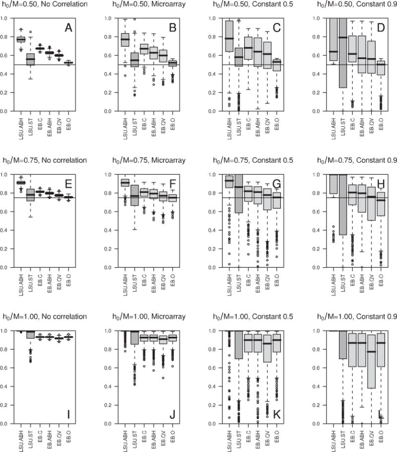
Boxplots of estimates h_0n/M of the proportion of true null hypotheses h₀/M (over A = 500 simulated data-sets), from FDR-controlling procedures LSU.ABH, LSU.ST, EB.C, EB.ABH, EB.QV, and EB.O, as summarized in Section 4.3.4. Results correspond to the following simulation parameters: sample size n = 250, number of null hypotheses M = 400, common alternative shift-parameter d_n(m) =2, $m\in {\mathcal{H}}_1$; proportion of true null hypotheses (h₀/M = 0.50, 0.75, 1.00) and correlation structure (σ* = “No correlation”, “Microarray”, “Constant 0.5”, “Constant 0.9”) indicated in the panel titles; B = 10,000 resampled test statistics and sets of true null hypotheses; A = 500 simulated datasets. The horizontal line indicates the true, unknown proportion of true null hypotheses, h₀/M. (Color version on website companion.)

5.1.2 Type I error control comparison

The Type I error properties of five non-oracle FDR-controlling procedures are illustrated in Figures 1 and 2 (M = 400 and 40 null hypotheses, respectively), for a range of nominal FDR levels α ∈ [0.01,0.20].

Figure 1. Simulation study: Type I error control comparison.

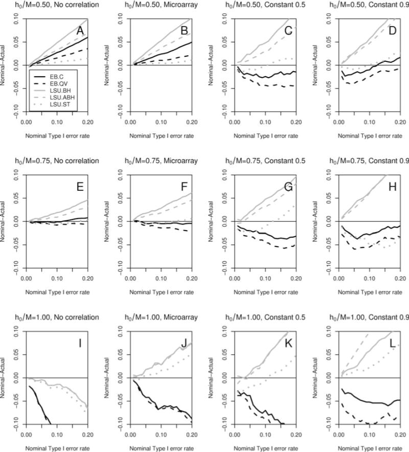
Plots of differences α − FDR(α) between nominal and actual Type I error rates vs. nominal Type I error level α ∈ [0.01, 0.20], for FDR-controlling procedures EB.C, EB.QV, LSU.BH, LSU.ABH, and LSU.ST, summarized in Table 1. Results correspond to the following simulation parameters: sample size n = 250, number of null hypotheses M = 400, common alternative shift parameter d_n(m) =2, $m\in {\mathcal{H}}_1$; proportion of true null hypotheses (h₀/M = 0.50, 0.75, 1.00) and correlation structure (σ* = “No correlation”, “Microarray”, “Constant 0.5”, “Constant 0.9”) indicated in the panel titles; B = 10,000 resampled test statistics and sets of true null hypotheses; A = 500 simulated datasets. Positive (negative) differences indicate (anti-) conservative behavior. (Color version on website companion.)

Figure 2. Simulation study: Type I error control comparison.

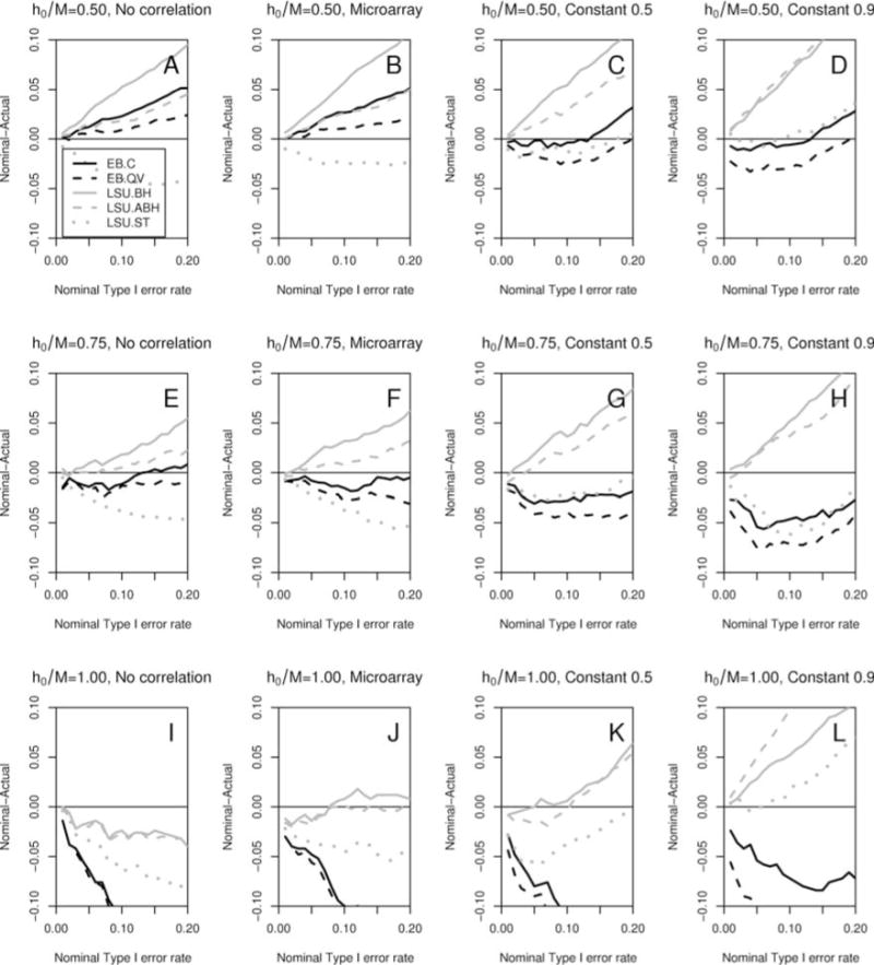
Plots of differences α − FDR(α) between nominal and actual Type I error rates vs. nominal Type I error level α ∈ [0.01, 0.20], for FDR-controlling procedures EB.C, EB.QV, LSU.BH, LSU.ABH, and LSU.ST, summarized in Table 1. Results correspond to the following simulation parameters: sample size n = 250, number of null hypotheses M = 40, common alternative shift parameter d_n(m) = 2, $m\in {\mathcal{H}}_1$; proportion of true null hypotheses (h₀/M = 0.50, 0.75, 1.00) and correlation structure (σ* = “No correlation”, “Microarray”, “Constant 0.5”, “Constant 0.9”) indicated in the panel titles; B = 10,000 resampled test statistics and sets of true null hypotheses; A = 500 simulated datasets. Positive (negative) differences indicate (anti-) conservative behavior. (Color version on website companion.)

Overall, procedures tend to be more conservative for smaller proportions of true null hypotheses h₀/M, with the resampling-based empirical Bayes procedures (EB.C and EB.QV) and Storey and Tibshirani’s (2003) linear step-up procedure LSU.ST remaining closer (in absolute value) to the target nominal Type I error level a (horizontal line) than the linear step-up procedures of Benjamini and colleagues (LSU.BH and LSU.ABH). The LSU.BH and LSU.ABH procedures tend to be conservative over the range of simulation parameters, while the empirical Bayes EB.C and EB.QV procedures and the Storey and Tibshirani (2003) LSU.ST procedure become anti-conservative with stronger correlation structures and higher proportions of true null hypotheses.

As expected, under no correlation, the classical linear step-up procedure LSU.BH of Benjamini and Hochberg (1995) becomes more conservative as the proportion of true null hypotheses h₀/M decreases (Figures 1 and 2, Panels A, E, and I). The adaptive procedures relax this conservatism.

The results for the empirical microarray correlation structure are similar to those for no correlation, although the empirical Bayes procedures are somewhat less conservative when compared to the linear step-up procedures (Figures 1 and 2, Panels B, F, and J).

Under constant correlation, the procedures of Benjamini and colleagues remain conservative. The LSU.ST procedure is generally anti-conservative, except for the extreme scenario with the complete null hypothesis (h₀/M = 1.00) and heavy correlation (σ* = 0.90) and some other scenarios for large nominal FDR levels α. The empirical Bayes procedures display anti-conservative behavior, particularly with a relaxed prior and as the proportion of true null hypotheses increases (Figures 1 and 2, Panels C, D, G, H, K, and L).

5.1.3 Power comparison

As argued in Section 4.3.3, fair power comparisons between multiple testing procedures are best performed by benchmarking power against actual, rather than nominal, Type I error rate (Figure 3).

Figure 3. Simulation study: Power comparison.

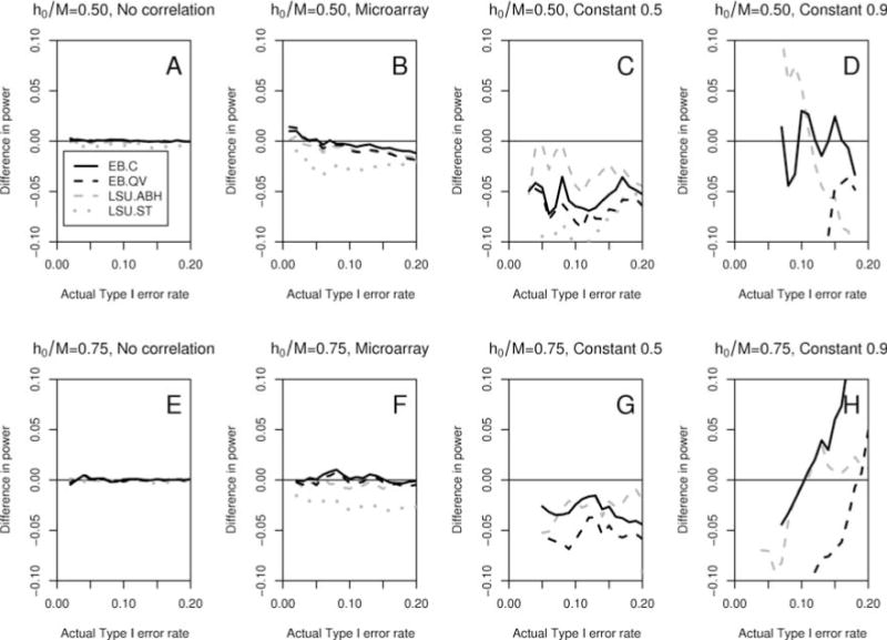
Plots of differences in power vs. actual Type I error rate, for FDR-controlling procedures EB.C, EB.QV, LSU.BH, LSU.ABH, and LSU.ST, summarized in Table 1, using LSU.BH as baseline. Results correspond to the following simulation parameters: sample size n = 250, number of null hypotheses M = 400, common alternative shift parameter d_n(m) =2, $m\in {\mathcal{H}}_1$; proportion of true null hypotheses (h₀/M = 0.50, 0.75) and correlation structure (σ* = “No correlation”, “Microarray”, “Constant 0.5”, “Constant 0.9”) indicated in the panel titles; B = 10,000 resampled test statistics and sets of true null hypotheses; A = 500 simulated datasets. Positive (negative) differences indicate greater (lower) power than the baseline LSU.BH procedure. (Color version on website companion.)

For the no correlation structure, no method is more powerful outright than the original linear step-up procedure LSU.BH of Benjamini and Hochberg (1995) (Figure 3, Panels A and E). In this case, all gains in power observed in Table 2 for the adaptive linear step-up procedures or resampling-based empirical Bayes procedures (when benchmarking against the nominal FDR, α = 0.05) are due to these procedures selecting less conservative cut-offs, with higher actual FDR, rather than being more powerful per se.

Under empirical microarray correlation, the empirical Bayes procedures (EB.C and EB.QV) are as powerful as standard linear step-up procedure LSU.BH, whereas the Storey and Tibshirani (2003) linear step-up LSU.ST procedure is slightly less powerful (Figure 3, Panels B and F).

In the constant correlation scenario, all procedures loose power relative to the Benjamini and Hochberg (1995) LSU.BH procedure, the largest loss occurring for the Storey and Tibshirani (2003) LSU.ST procedure (Figure 3, Panels C, D, G, and H, with LSU.ST being outside the plotting area in some cases of extreme loss of power).

5.2 Estimation of the proportion of true null hypotheses

The properties of six estimators of the proportion h₀/M of true null hypotheses are illustrated in Figure 4, using boxplots over A simulated datasets (Section 4.3.4).

Overall, the estimators tend to be conservatively biased, with decreasing bias for higher proportions of true null hypotheses. Variability tends to increase with increasing correlation levels.

The LSU.ABH estimator, used in the adaptive linear step-up procedure of Benjamini and Hochberg (2000), is consistently the most conservative. The LSU.TST estimator (α = 0.05, 0.10), from the two-stage linear step-up procedure of Benjamini et al. (2006), is similar to the LSU.ABH estimator, with a slightly less conservative bias for the higher nominal Type I error level α = 0.10 (results not shown). These observations reinforce earlier findings that the procedures of Benjamini and colleagues are capable of maintaining desired levels of Type I error control across a variety of conditions (Figures 1 and 2 and Table 2).

As expected, the q-value-based empirical Bayes estimators of h₀=M become less conservative as the estimated prior π_0n is relaxed. These estimators are still conservatively biased, although the lower tails of their distributions dip below the true value h₀=M more frequently as the correlation and/or proportion of true null hypotheses increase.

Although often the least biased among non-oracle estimators of h₀=M, the LSU.ST estimator, from the adaptive linear step-up procedure of Storey and Tibshirani (2003), is by far the most variable. In particular, for a small number of hypotheses M = 40 and/or constant correlation structure σ*, the qvalue software returns errors for roughly 1–5% (σ* = 0.50) and 20–30% (σ* = 0.90) of simulated datasets, indicating that a negative estimate of the proportion h₀=M is produced. Moreover, as noted by Benjamini et al. (2006), the LSU.ST method can yield estimates that exceed one. Specifically, for M = 400 hypotheses and h₀/M = 0.75, estimates of h₀/M had to be bounded by one for 10 (out of A = 500, i.e., 2.0%) simulated datasets with no correlation among variables, 46 (9.2%) datasets with empirical microarray correlation structure, 143 (28.6%) datasets with constant correlation structure (σ* = 0.50), and 188 (37.6%) datasets with constant correlation structure (σ* = 0.90).

Estimators of h₀=M are slightly less conservative for a smaller number of hypotheses M = 40, but vary between the M = 40 and M = 400 scenarios by only ca. 1% for empirical Bayes EB.C, EB.O, EB.ABH, and EB.QV estimators, ca. 2–3% for Benjamini and Hochberg (2000) LSU.ABH estimator, and ca. 4–6% for Storey and Tibshirani (2003) LSU.ST estimator (results not shown).

5.3 Additional simulation results

Please refer to the website companion.

6 Discussion

6.1 Summary

We have proposed resampling-based empirical Bayes procedures for controlling generalized tail probability error rates, gTP(q, g) = Pr (g(V_n, Sn) > q), and generalized expected value error rates, gEV(g) = E[g(V_n, S_n)], for arbitrary functions g(V_n, S_n) of the numbers of false positives V_n and true positives S_n.

The simulation study of Sections 4 and 5 illustrates the competitive Type I error and power properties of the resampling-based empirical Bayes procedures when compared to widely-used FDR-controlling linear step-up procedures. These results for FDR control are consistent with previous results for TPPFP control in the original article of von der Laan et al. (2005).

For a variety of testing scenarios, the resampling-based empirical Bayes approach exhibits Type I error and power properties intermediate between those of the linear step-up procedures of Benjamini and colleagues and Storey and colleagues (Figures 1–3, Table 2). Specifically, empirical Bayes procedures control the false discovery rate less conservatively than the classical Benjamini and Hochberg (1995) procedure and adaptive versions thereof (Benjamini and Hochberg, 2000, Benjamini et al., 2006), with, as for the Storey and Tibshirani (2003) procedure, the risk of anti-conservative behavior for heavy correlation structures and a high proportion of true null hypotheses. The empirical Bayes procedures tend to be more powerful than the q-value procedure of Storey and Tibshirani (2003), particularly for microarray-like correlation structures, which have been presented in the literature as exhibiting potentially weak dependence or dependence in finite blocks (Storey, 2002; Storey and Tibshirani, 2003; Storey et al., 2004).

The simulation study indicates that gains in power can be achieved by the empirical Bayes procedures when using a data-adaptive prior π_0n to estimate the local q-values π_0n(T_n(m)). The decision to deviate from the most conservative prior (π_0n = 1), however, should be guided by prior knowledge regarding the proportion of true null hypotheses as well as the level of correlation between test statistics. In many applications, the anti-conservative bias occurring in extreme simulation conditions will either not be present or may be of minor practical significance.

The local q-values, used to generate the random guessed sets of true null hypotheses in the empirical Bayes procedures, provide estimators of the proportion of true null hypotheses that tend to be less conservatively biased than the Benjamini and Hochberg (2000) estimator and less variable than the Storey and Tibshirani (2003) estimator.

Of course, an issue in presenting any resampling-based procedure is the trade-off between gains in accuracy and extra computational cost. As shown in this study, for testing scenarios with no correlation and a large proportion of true null hypotheses, the empirical Bayes procedures do not improve upon the linear step-up methods of Benjamini and colleagues. If Type I error control is the primary concern, then these simpler procedures are probably the better choice. However, when the goal is to reject a larger number of hypotheses, while still maintaining adequate Type I error control, then the empirical Bayes procedures are strong contenders under various levels of correlation.

6.2 Distribution for the guessed sets of true null hypotheses

The simulation study of Sections 4 and 5 reveals anti-conservative behavior of empirical Bayes Procedure 3.1 for testing scenarios with a high proportion of true null hypotheses and, in particular, for the complete null hypothesis (h₀/M = 1). As argued below and in greater detail on the website companion, this failure to control Type I errors is a limitation not of the empirical Bayes approach in general, but rather of a specific model used to generate the guessed sets of true null hypotheses, namely, the mixture model described in Section 3.3.

Recall that the proposed resampling-based empirical Bayes Procedure 3.1 has the following two main ingredients.

• A null distribution Q₀ (or estimator thereof, Q_0n) for M-vectors of null test statistics T_0n.

• A distribution $Q_0^{\mathcal{H}}$ (or estimator thereof, $Q_{0n}^{\mathcal{H}}$) for random guessed sets of true null hypotheses ${\mathcal{H}}_{0n}$.

The asymptotic Type I error control results of Dudoit and van der Laan (2008, Theorem 7.2) are derived under a number of assumptions regarding these two distributions. In particular, one of the assumptions concerns consistency of the guessed sets of true null hypotheses H_0n: for almost every (P_n : n ≥ 1), ${\lim }_{n\to \infty }{\mathcal{H}}_{0n}={\mathcal{H}}_0$.

For the resampling-based empirical Bayes procedures considered in the simulation study of Sections 4 and 5, the guessed sets of true null hypotheses ${\mathcal{H}}_{0n}^b$ are generated from a distribution $Q_{0n}^{\mathcal{H}}$ which is based on a common marginal non-parametric mixture model for the test statistics (Section 3.3). In practice, for testing problems with a large number of hypotheses M and some false null hypotheses h₀ < M, we have found this model to yield good Type I error control and power properties. Other authors have recommended this model in the context of FDR-controlling procedures (Efron et al., 2001; Storey and Tibshirani, 2003). However, when all M null hypotheses are true, i.e., h₀ = M, the estimator ${\mathcal{H}}_{0n}$ of ${\mathcal{H}}_0$ does not satisfy the consistency assumption of Dudoit and van der Laan (2008, Theorem 7.2). In particular, the guessed sets H_0n tend to be “too small”, i.e., ${\mathcal{H}}_{0n}\subseteq {\mathcal{H}}_0=\{1,\dots ,M\}$, and, as a result, Procedure 3.1 tends to be anti-conservative. We expect this bias to be most severe in the case of a small number of hypotheses M. Thus, the mixture model-based estimator ${\mathcal{H}}_{0n}$ of Section 3.3 should only be used in settings in which one expects some false null hypotheses (h₀ < M) or M is very large. Furthermore, in terms of power considerations, this estimator is reasonable only when one expects the test statistics for the false null hypotheses to have similar marginal distributions.

Note that similar anti-conservative behavior is observed for Storey and Tibshirani’s (2003) linear step-up procedure, which is also related to the mixture model of Section 3.3.

We wish to stress that Procedure 3.1 and the associated results in Theorem 7.2 of Dudoit and van der Laan (2008) are not tied in any way to the mixture model of Section 3.3 or any other model for the distribution $Q_{0n}^{\mathcal{H}}$ of the guessed sets of true null hypotheses ${\mathcal{H}}_{0n}$. It would therefore be of interest, from both a theoretical and practical point of view, to develop consistent estimators of ${\mathcal{H}}_0$, that satisfy the assumptions of Dudoit and van der Laan (2008, Theorem 7.2) and, in particular, can adapt to the complete null hypothesis setting in which h₀ = M.

6.3 Ongoing efforts

Ongoing efforts include further investigating the distribution $Q_{0n}^{\mathcal{H}}$ for the guessed sets of true null hypotheses, in order to guarantee proper Type I error control by the empirical Bayes procedures for a wider range of testing scenarios. In particular, we are interested in developing less biased estimators of the density ratio f₀/f in the local q-value function, as diagnostic tests suggest that f₀/f is a critical quantity regarding Type I error control.

We are also considering improvements to the estimator of the gTP and gEV error rates in Eq. (27), which is used to select test statistic cut-offs that satisfy the Type I error constraint of Eq. (38). In the common-cut-off case and for testing scenarios with a large proportion of true null hypotheses h₀/M, we have noted that the current estimator

$${\widehat{\mathrm{\theta }}}_n({\mathrm{\gamma }}^{(M)})=\frac{1}{B}{\displaystyle \sum _{b=1}^B\tilde{G}({\mathrm{\gamma }}^{(M)};{\mathcal{H}}_{0n}^b,T_{0n}^b,T_n),}$$

of the Type I error function ${\mathrm{\theta }}_n\left({\mathrm{\gamma }}^{(M)}\right)=E[\tilde{G}{\mathrm{\gamma }}^{(M)};{\mathcal{H}}_0,T_n,T_n]$, can be anti-conservatively biased and variable, i.e., non-monotonic in the common cut-off γ. This is especially problematic for the complete null hypothesis (h₀/M = 1), where the false discovery rate coincides with the family-wise error rate and one would therefore like estimators of these two error rates to be nearly equal and monotonic in the common cut-off γ. Smoothing or enforcing monotonicity constraints on the estimator ${\widehat{\mathrm{\theta }}}_n\left({\mathrm{\gamma }}^{(M)}\right)$ may alleviate the anti-conservative bias.

Finally, we are implementing the proposed multiple testing procedures in the R package mult-test, released as part of the Bioconductor Project.

6.4 Conclusion

We wish to stress the benefits and generality of the proposed resampling-based empirical Bayes methodology.

• General Type I error rates. It can be used to control a broad class of Type I error rates, defined as tail probabilities and expected values of arbitrary functions g(V_n, S_n) of the numbers of false positives V_n and true positives S_n. As discussed in Dudoit and van der Laan (2008, Section 7.8), the approach can be further extended to control other parameters of the distribution of functions g(V_n, S_n). Researchers can therefore select from a wide library of Type I error rates for subject-matter-relevant measures of false positives and control these error rates at little additional computational cost, using the same resampled pairs $(T_{0n}^b,{\mathcal{H}}_{0n}^b)$: e.g., generalized family-wise error rate, tail probabilities for the proportion of false positives.

• General distributions for the test statistics. Unlike most MTPs controlling the proportion of false positives, it is based on a test statistics joint null distribution and provides Type I error control in testing problems involving general data generating distributions, with arbitrary dependence structures among variables.

• Power. Gains in power are achieved by deriving rejection regions based on guessed sets of true null hypotheses and null test statistics randomly sampled from joint distributions that account for the dependence structure of the data.

• Genericness and modularity. It is generic and modular, in the sense that it can be applied successfully to any distribution pair $(Q_{0n},Q_{0n}^{\mathcal{H}})$, for the null test statistics and guessed sets of true null hypotheses, provided $(Q_{0n},Q_{0n}^{\mathcal{H}})$ satisfy the assumptions of Dudoit and van der Laan (2008, Theorem 7.2). The common marginal non-parametric mixture model of Section 3.3 has the attractive property that it does not assume independence of the test statistics. However, it is only one among many reasonable working models for the distribution of the guessed sets of true null hypotheses.

In conclusion, the Type I error and power trade-off achieved by the resampling-based empirical Bayes procedures under a variety of testing scenarios (with varying degrees of correlation) allows this approach to be competitive with or outperform the Storey and Tibshirani (2003) linear step-up procedure, as an alternative to the classical Benjamini and Hochberg (1995) procedure.

Software

The multiple testing procedures proposed in Dudoit and van der Laan (2008) and related articles (Birkner et al., 2005; Dodoit et al., 2004a, b; van der Laan et al., 2004b, a, 2005; van der Laan and Hubbard, 2006; Pollard et al., 2005a, b; Pollard and van der Laan, 2004) are implemented in the R package multtest, released as part of the Bioconductor Project, an open-source software project for the analysis of biomedical and genomic data (Dudoit and van der Laan (2008, Section 13.1); Pollard et al. (2005b); www.bioconductor.org).

The simulation study was performed in R (Release 2.5.1), using the following packages: MASS (Version 7.2–34), multtest (Version 1.16.0), qvalue (Version 1.1), and golubEsets (Version 1.4.3).

References

- Benjamini Y, Hochberg Y. Controlling the false discovery rate: A practical and powerful approach to multiple testing. Journal of the Royal Statistical Society, Series B. 1995;57:289–300. [Google Scholar]
- Benjamini Y, Hochberg Y. On the adaptive control of the false discovery rate in multiple testing with independent statistics. Journal of Educational and Behavioral Statistics. 2000;25:60–83. [Google Scholar]
- Benjamini Y, Krieger AM, Yekutieli D. Adaptive linear step-up false discovery rate controlling procedures. Biometrika. 2006;93:491–507. [Google Scholar]
- Benjamini Y, Yekutieli D. The control of the false discovery rate in multiple testing under dependency. Annals of Statistics. 2001;29:1165–1188. [Google Scholar]
- Birkner MD, Pollard KS, van der Laan MJ, Dudoit S. Multiple testing procedures and applications to genomics. Division of Biostatistics, University of California; Berkeley, Berkeley, CA: 2005. pp. 94720–7360. (Technical Report 168). [Google Scholar]
- Dudoit S, van der Laan MJ. Multiple Testing Procedures with Applications to Genomics. Springer; New York: 2008. (Springer Series in Statistics). [Google Scholar]
- Dudoit S, van der Laan MJ, Birkner MD. Multiple testing procedures for controlling tail probability error rates. Division of Biostatistics, University of California; Berkeley, Berkeley, CA: 2004a. pp. 94720–7360. (Technical Report 166). [Google Scholar]
- Dudoit S, van der Laan MJ, Pollard KS. Multiple testing. Part I. Single-step procedures for control of general Type I error rates. Statistical Applications in Genetics and Molecular Biology. 2004b;3 doi: 10.2202/1544-6115.1040. Article 13. [DOI] [PubMed] [Google Scholar]
- Efron B, Tibshirani R, Storey JD, Tusher V. Empirical Bayes analysis of a microarray experiment. Journal of the American Statistical Association. 2001;96:1151–1160. [Google Scholar]
- Genovese CR, Wasserman L. Exceedance control of the false discovery proportion. Department of Statistics, Carnegie Mellon University; Pittsburgh, PA 15213: 2004a. (Technical Report 807). [Google Scholar]
- Genovese CR, Wasserman L. A stochastic process approach to false discovery control. Annals of Statistics. 2004b;32:1035–1061. [Google Scholar]
- Golub TR, Slonim DK, Tamayo P, Huard C, Gaasenbeek M, Mesirov JP, Coller H, Loh M, Downing JR, Caligiuri MA, Bloomfield CD, Lander ES. Molecular classification of cancer: Class discovery and class prediction by gene expression monitoring. Science. 1999;286:531–537. doi: 10.1126/science.286.5439.531. [DOI] [PubMed] [Google Scholar]
- Lehmann EL, Romano JP. Generalizations of the familywise error rate. Annals of Statistics. 2005;33:1138–1154. [Google Scholar]
- Pollard KS, Birkner MD, van der Laan MJ, Dudoit S. Test statistics null distributions in multiple testing: Simulation studies and applications to genomics. Journal de la Société Française de Statistique. 2005a;146:77–115. Numéro double spécial Statistique et Biopuces. [Google Scholar]
- Pollard KS, Dudoit S, van der Laan MJ. Multiple testing procedures: The multtest package and applications to genomics. In: Gentleman RC, Carey VJ, Huber W, Irizarry RA, Dudoit S, editors. Bioinformatics and Computational Biology Solutions Using R and Bioconductor. Springer; New York: 2005b. pp. 249–271. chapter 15. [Google Scholar]
- Pollard KS, van der Laan MJ. Choice of a null distribution in resampling-based multiple testing. Journal of Statistical Planning and Inference. 2004;125:85–100. [Google Scholar]
- Storey JD. A direct approach to false discovery rates. Journal of the Royal Statistical Society, Series B. 2002;64:479–498. [Google Scholar]
- Storey JD, Taylor JE, Siegmund DO. Strong control, conservative point estimation and simultaneous conservative consistency of false discovery rates: A unified approach. Journal of the Royal Statistical Society, Series B. 2004;66:187–205. [Google Scholar]
- Storey JD, Tibshirani R. Statistical significance for genomewide studies. Proceedings of the National Academy of Sciences. 2003;100:9440–9445. doi: 10.1073/pnas.1530509100. [DOI] [PMC free article] [PubMed] [Google Scholar]
- van der Laan MJ, Birkner MD, Hubbard AE. Empirical Bayes and resampling based multiple testing procedure controlling tail probability of the proportion of false positives. Statistical Applications in Genetics and Molecular Biology. 2005;4 doi: 10.2202/1544-6115.1143. Article 29. [DOI] [PubMed] [Google Scholar]
- van der Laan MJ, Dudoit S, Pollard KS. Augmentation procedures for control of the generalized family-wise error rate and tail probabilities for the proportion of false positives. Statistical Applications in Genetics and Molecular Biology. 2004a;3 doi: 10.2202/1544-6115.1042. Article 15. [DOI] [PubMed] [Google Scholar]
- van der Laan MJ, Dudoit S, Pollard KS. Multiple testing. Part II. Step-down procedures for control of the family-wise error rate. Statistical Applications in Genetics and Molecular Biology. 2004b;3 doi: 10.2202/1544-6115.1041. Article 14. [DOI] [PubMed] [Google Scholar]
- van der Laan MJ, Hubbard AE. Quantile-function based null distribution in resampling based multiple testing. Statistical Applications in Genetics and Molecular Biology. 2006;5 doi: 10.2202/1544-6115.1199. Article 14. [DOI] [PubMed] [Google Scholar]
Associated Data
This section collects any data citations, data availability statements, or supplementary materials included in this article.