Dynamic Target Match Signals in Perirhinal Cortex Can Be Explained by Instantaneous Computations That Act on Dynamic Input from Inferotemporal Cortex

Abstract

Finding sought objects requires the brain to combine visual and target signals to determine when a target is in view. To investigate how the brain implements these computations, we recorded neural responses in inferotemporal cortex (IT) and perirhinal cortex (PRH) as macaque monkeys performed a delayed-match-to-sample target search task. Our data suggest that visual and target signals were combined within or before IT in the ventral visual pathway and then passed onto PRH, where they were reformatted into a more explicit target match signal over ∼10–15 ms. Accounting for these dynamics in PRH did not require proposing dynamic computations within PRH itself but, rather, could be attributed to instantaneous PRH computations performed upon an input representation from IT that changed with time. We found that the dynamics of the IT representation arose from two commonly observed features: individual IT neurons whose response preferences were not simply rescaled with time and variable response latencies across the population. Our results demonstrate that these types of time-varying responses have important consequences for downstream computation and suggest that dynamic representations can arise within a feedforward framework as a consequence of instantaneous computations performed upon time-varying inputs.

Introduction

Finding sought objects and switching between targets requires the flexible combination of visual information about the content of a currently viewed scene with working memory information about the identity of a sought target. These signals are thought to be combined within mid-to-higher stages of the ventral visual pathway [i.e., within V4 and inferotemporal cortex (IT); Fig. 1], where the responses of neurons are modulated by changing both the identity of a visual stimulus and the identity of a sought target (Haenny et al., 1988; Maunsell et al., 1991; Eskandar et al., 1992; Gibson and Maunsell, 1997; Liu and Richmond, 2000; Chelazzi et al., 2001; Bichot et al., 2005). The resulting target-modulated visual signals are then thought to be transformed into a “target match” signal that explicitly reports whether a currently viewed scene contains a target via nonlinear computations that are implemented within perirhinal cortex (PRH; Chelazzi et al., 1993; Miller and Desimone, 1994; Pagan et al., 2013) and prefrontal cortex (Miller et al., 1996).

Figure 1.

Untangling target match signals. Left, Previous results suggest that during visual target search, visual and working memory signals are combined within or before IT along the ventral visual pathway in a nonlinearly separable or tangled fashion, followed by computations in PRH that untangle target match information such that it is more accessible to a linear population readout. Right, Each point depicts a hypothetical population response, consisting of a vector of the spike count responses to a single condition on a single trial. Clouds of points depict the predicted dispersion across repeated presentations of the same condition due to trial-by-trial variability. The different shapes depict the hypothetical responses to different images and the two shades (black, gray) depict the hypothetical responses to target matches and distractors, respectively. A target-switching task (such as the delayed-match-to-sample task, Fig. 2) requires discriminating the same objects presented as target matches and as distractors. In a tangled representation (bottom), a nonlinear decision boundary (corresponding to a nonlinear population readout) is required to separate these two groups whereas an untangled representation (top) can be read out with a linear decision boundary (corresponding to a linear population readout). As reported by Pagan et al. (2013), target match signals are more tangled in IT and more untangled in PRH.

The computations required to create a target match signal can be envisioned as nonlinear conjunctions or “and-like” computations between visual and working memory signals (i.e., I am looking at my car keys “and” I am looking for my car keys). Evolution in the responses of neurons during and-like computations has been reported not only during target search (Chelazzi et al., 1993, 2001), but also for computations involved in motion processing (Pack and Born, 2001; Smith et al., 2005) and object recognition (Brincat and Connor, 2006). Specifically, these studies have revealed a delay between the time signals arrive within a brain area and the time that conjunction information appears on the order of tens of milliseconds. These delays have been attributed to the time required for recurrent circuits within the brain area performing the computation to execute it (Brincat and Connor, 2006), possibly via a biased, competitive process (Chelazzi et al., 1993).

Here we report a similar phenomenon, but one in which delays in the emergence of conjunction information can be attributed to computations that are instantaneous and fixed but act on an input representation that changes over time. More specifically, we found that during a delayed-match-to-sample target search task, visual and working memory signals were partially represented in PRH as separate signals that then evolved into an “and-like” target match signal over ∼10–15 ms. These dynamics were not simply inherited from the IT inputs and, surprisingly, they did not require proposing dynamic computation within PRH itself. Rather, our data were well accounted for by a description in which the “and-like” computations that produce target match signals in PRH were gradually implemented across at least two processing stages: one that combined visual and working memory signals within or before IT to form a partially nonlinearly separable and time-varying representation, followed by computations in PRH that instantaneously reformatted the input arriving from IT to produce a more explicit target match signal.

Materials and Methods

The data reported here are the same data described by Pagan et al. (2013). The experimental procedures involved in collecting the data are described in detail in that report and are summarized here. Experiments were performed on two naive adult male rhesus macaque monkeys (Macaca mulatta) with implanted head posts and recording chambers. All procedures were performed in accordance with the guidelines of the University of Pennsylvania Institutional Animal Care and Use Committee.

All behavioral training and testing were performed using standard operant conditioning (juice reward), head stabilization, and high-accuracy, infrared video eye tracking. Monkeys performed a delayed-match-to-sample task (Fig. 2a). Monkeys initiated each trial by fixating a small dot. After a 250 ms delay, an image indicating the target was presented, followed by a random number (0–3, uniformly distributed) of distractors, and then the target match. Each image was presented for 400 ms, followed by a 400 ms blank. Monkeys were required to maintain fixation throughout the distractors and make a saccade to a response dot located 7.5 degrees below fixation after 150 ms following target match onset but before the onset of the next stimulus to receive a reward. The same four images were used during all the experiments. Approximately 25% of trials included the repeated presentation of the same distractor with zero or one intervening distractors of a different identity. Behavioral performance was high (monkey 1 = 94%; monkey 2 = 92%). The same target remained fixed within short blocks of ∼1.7 min that included an average of 9 correct trials. Within each block, four presentations of each condition (for a fixed target) were collected and all four target blocks were presented within a “metablock” in pseudorandom order before reshuffling. A minimum of 5 metablocks in total (20 correct presentations for each experimental condition) were collected. The main components of this experimental design included 16 different conditions that could be envisioned as existing within a 4 × 4 matrix defined by each of the four images presented as a visual stimulus in the context of looking for each of the four images as a target (Fig. 2b). This matrix includes four target match conditions, which fall along the diagonal of this matrix, and 12 “distractor” conditions, which fall off the matrix diagonal.

Figure 2.

The delayed-match-to-sample task. a, Monkeys performed a delayed-match-to-sample task that required them to treat the same four images as target matches and as distractors in different blocks of trials. Monkeys initiated a trial by fixating a small dot. After a delay, an image appeared indicating the identity of the target, followed by a random number (0–3, uniformly distributed) of distractors, and then the target match. Monkeys were required to maintain fixation throughout the distractors and make a downward saccade when the target appeared to receive a reward. Approximately 25% of trials included the repeated presentation of the same distractor with zero or one intervening distractor of a different identity, similar to Miller and Desimone (1994). b, Each of four images were presented in all possible combinations as a visual stimulus (looking at), and as a target (looking for), resulting in a four-by-four response matrix. In these matrices, conditions corresponding to the same visual input correspond to columns, conditions corresponding to the same working memory or target input correspond to rows, and target matches fall along the diagonal, while distractors fall off the diagonal. The type of matrix structure required to differentiate other types of conditions (e.g., looking at image 2 and for image 4) are referred to as non-diagonal cognitive.

Both IT and PRH were accessed via a single recording chamber in each animal. Chamber placement was guided by anatomical magnetic resonance images and later verified physiologically by the locations and depths of gray and white matter transitions. The region of IT recorded was located on both the ventral superior temporal sulcus and the ventral surface of the brain, over a 4 mm medial-lateral region located lateral to the anterior middle temporal sulcus (AMTS) that spanned 14–17 mm anterior to the ear canals (Liu and Richmond, 2000; Rust and DiCarlo, 2010). The region of PRH recorded was located medial to the AMTS and lateral to the rhinal sulcus and extended over a 3 mm medial-lateral region located 19–22 mm anterior to the ear canals (Liu and Richmond, 2000). We recorded neural activity via a combination of glass-coated tungsten single electrodes (Alpha Omega) and 16 and 24 channel U-probes with recording sites arranged linearly and separated by 150 μm spacing (Plexon). Continuous, wideband neural signals were amplified, digitized at 40 kHz, and stored via the OmniPlex Data Acquisition System (Plexon). We performed all spike sorting manually offline using commercially available software (Plexon).

Responses were only analyzed on correct trials. Target matches that were presented after the maximal number of distractors (n = 3) occurred with 100% probability and were discarded from the analysis. The response of each neuron was measured as the spike count in time bins 25 ms wide and sampled at 1 ms intervals aligned to the onset of each visual image. In some of our analyses (described below), we assume that trial-by-trial response variability arose from a Poisson process, as we found this to be a good account of our data. For each neuron at each bin position (−50 to 250 ms relative to stimulus onset), we estimated the Fano factor by fitting the relationship between the mean and variance of spike counts for each of the 16 experimental conditions (Rust et al., 2002). Grand mean Fano factor estimates averaged across all neurons and all windows (based on spike counts in 25 ms windows with shifts of 1 ms) was 1.01 in both IT and PRH. Similar to other reports (Churchland et al., 2010), we found a small but reliable decrease in Fano factor following stimulus onset (e.g., in IT, average Fano factor dropped from a maximum mean ± SD of 1.06 ± 0.15 at −50 ms to 0.94 ± 0.13 at 112 ms).

Population performance

To measure the amount and format of information available in the IT and PRH populations to discriminate target matches and distractors, we performed two cross-validated classification analyses: a linear readout and an ideal observer readout (Pagan et al., 2013). For both analyses, we considered the spike count responses of a population of N neurons (where N = 164 in IT and PRH) to each condition as a population “response vector” x with dimensionality equal to Nx1. Our experimental design resulted in 4 target match conditions and 12 distractor conditions; on each iteration we randomly selected 1 distractor condition from each image (for a total of 4 distractor conditions) to avoid artificial overestimations of classifier performance that could be produced by taking the prior distribution into account (e.g., scenarios in which the answer is more likely to be distractor than target match). The linear readout (Fig. 3a) amounted to finding the linear hyperplane that would best separate the population response vectors corresponding to all of the target match conditions from the response vectors corresponding to all of the distractor conditions and took the form:

where w is an Nx1 vector describing the linear weight applied to each neuron and b is a scalar value that offsets the hyperplane from the origin and acts as a threshold. The population classification of a test response vector was assigned to a target match when f(x) exceeded zero and was classified as a distractor otherwise. The hyperplane and threshold for each classifier were determined by a support vector machine (SVM) procedure using the LIBSVM library (http://www.csie.ntu.edu.tw/∼cjlin/libsvm/) with a linear kernel, the C-SVC algorithm, and cost (C) set to 0.1.

Figure 3.

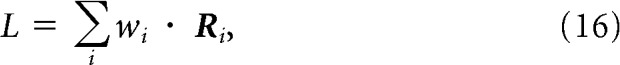
Target match signals are gradually untangled in PRH. Comparison of the temporal evolution of the performance of an ideal observer classifier, to assess the amount of total target match information, and a linear classifier, to assess the amount of target match information that was accessible to a linear readout. Cross-validated performance was computed with spike counts within 25 ms bins sampled at 1 ms intervals. In all panels, the horizontal dotted line indicates chance performance and n indicates the number of neurons included in each population. a, Performance for the data pooled across both monkeys; shaded region indicates SE of performance (the y-axis). b, Left, The same data in a shown from 0 to 140 ms to more closely examine the delay but with SE computed for time (the x-axis). Right, The same analysis performed on a subset of trials in which performances were matched in magnitude from 135 to 140 ms (see Materials and Methods). c, The same analysis presented in b, right, but applied to the data from each monkey individually. d, Left, As a control analysis, direct measures of linear and nonlinear performance using two classifiers matched for numbers of parameters (see Materials and Methods). Right, The ratio of chance-corrected linear and nonlinear performance computed from the plots on the right where the ratio was determined for each time bin as (linear—0.5)/(nonlinear—0.5).

Our “ideal observer” readout (Fig. 3a) was designed to be “ideal” in the sense that its performance was limited by the amount of overlap in the trial-by-trial responses to target matches and distractors (i.e., it is optimal under the assumption of Poisson trial-by-trial variability) but not by the complexity of the decision boundary required to connect the multiple target match conditions and parse those from the multiple distractor conditions. We note that the ideal observer is not proposed as a neurally plausible readout, but rather as a method to estimate the maximum achievable performance using an arbitrarily complex readout. To distinguish it from readouts that impose a particular decision boundary (i.e., “linear”). we refer to it as a measure of “total” information. Importantly, this ideal observer will perform well under a range of circumstances in which complete information for this task exists (e.g., at one extreme, a population of individual neurons that each convey large amounts of linearly separable target match information; and at the other extreme, a population that contains visual and working memory signals in separate subpopulations of neurons). Additionally, this ideal observer will fail under conditions in which target match information is incomplete (e.g., a population that contains purely “visual” or “working memory” neurons alone). To determine the ideal observer readout, we computed the average spike count response r_uc of each neuron u to each condition c. The likelihood that a test response k arose from a particular condition for a neuron was computed as the Poisson probability density:

When applied to our model responses (see Materials and Methods, Model Structure), the Poisson probability density was extended to continuous responses by replacing the factorial with the gamma function (note that this formula is equivalent to Eq. 2 when k is an integer):

The likelihood that a test response vector x arose from each condition c for the population was computed as the product of the likelihoods for the individual neurons:

where x_u indicates the response of unit u on a single trial. Finally, we computed the likelihood that a test response vector arose from the category “target match” versus the category “distractor” as the mean of the likelihoods for target matches and distractors, respectively:

The population classification was assigned to the category with the higher likelihood.

For both types of classifiers, we computed cross-validated performance by randomly assigning 50% of our data (10 repeats) to compute the representation (“training set”) and testing with the remaining 50% of our data (10 repeats). To compute performance mean and SE, we performed a resampling procedure in which we randomly assigned repeats without replacement for training and testing. To combine the responses of neurons recorded in different sessions into a pseudopopulation, on each bootstrap iteration we shuffled the trial pairings between neurons to destroy any (artificial) trial-by-trial correlation structure. The readout was trained separately for each time point, but across different time points for the same neuron, we always analyzed data from the same experimental trials. We performed 3000 resampling iterations for each time point. Estimates of the mean and SE of performance at each time point were obtained by computing the mean and SD across bootstrap iterations (Fig. 3a).

To compute latency estimates for each type of classification (i.e., the latency for performance to reach a criterion; Fig. 3b,c), we considered the performance values p for all time points t on one bootstrap iteration and we fit a 12th-order polynomial to those data by minimizing mean square error:

(i.e., the function polyfit in Matlab). We used the resulting function to compute the latency values that corresponded to a range of criteria (i.e., the first time points that corresponded to performance values ranging from 0.55 to 0.875), although we could not estimate latencies on bootstrap iterations in which a criterion exceeded the maximum of the fitted function. We computed the latency mean and SE for each criterion as the mean and SD across these latency estimates. We computed the p-value for each criterion by considering pairs of latencies for the ideal observer and linear classifier and determining the fraction of those pairs for which the difference was flipped in sign relative to the actual difference between the means of the full dataset (i.e., the fraction of bootstrap iterations in which the ideal observer classification latency was larger than the linear classification latency; Efron and Tibshirani, 1994). Additionally, we determined the degree to which smaller-magnitude linear classifier performance could account for its longer latency relative to ideal observer performance by selecting the subset of bootstrap iterations on which ideal observer and linear classifier performance had the same distribution of magnitudes within a window of 135–140 ms, and we then calculated latencies on those magnitude-matched trials (Fig. 3b,c). Specifically, we performed a histogram equalization in which we computed histograms of performance averaged from 135 to 140 ms for both classifiers, and within each histogram bin, we randomly selected the same number of entries from each distribution. We then used the data from earlier time points on the same trials as these entries to calculate the mean and SEs for latencies as described above.

By design, our ideal observer classifier (designed to measure total information) is capable of retrieving a more complex decision boundary than the linear classifier (i.e., because linear is a subset of total). This is reflected in the larger number of degrees of freedom available to the ideal observer. Specifically, the number of ideal observer degrees of freedom is equal to the number of neurons multiplied by the number of discriminated conditions (i.e., 164 * 8, given that 4 matches and a subset of 4 distractors were discriminated on each bootstrap iteration of the classification procedure as described above), whereas the number of linear classifier degrees of freedom is equal to the number of neurons (i.e., 164). Because we indirectly infer the time course of nonlinearly separable information by comparing ideal observer and linear classifier performances, we designed a control analysis to evaluate whether differences in the numbers of parameters led to a spurious interpretation of our results. To do this, we developed a new linear and nonlinear classifier designed to measure each of these quantities directly and with the same number of parameters. The approach we took is analogous to a polynomial expansion of the classifier readout rule, where the first term corresponds to a linear classifier that captures differences between the mean population responses, and the second term corresponds to a nonlinear (quadratic) classifier chosen to maximize the difference between the variances of the population responses. Specifically, this linear classifier operates by maximizing the distance between the mean response across all matches and the mean response across all distractors, and was computed as the difference between the population response vector averaged across all matches and the population response vector averaged across all distractors (for the training data). Next, a threshold was computed via a brute-force search as the value that maximizes the fraction of correct classifications of matches and distractors in the training data. In contrast, the nonlinear classifier operates by projecting the training data onto the axis that maximizes the difference between the variance in the response across all matches and the variance in the response across all distractors, and this vector was computed from the eigendecomposition of the difference between the covariance matrices for matches and for distractors computed from the training data; this nonlinear classifier was taken as the eigenvector with the maximum absolute eigenvalue. After the population responses were projected along this axis, they were squared (which acts to convert these variance differences into mean differences) and a final threshold was computed as the value that maximized the fraction of correct classifications of matches and distractors in the training data. We note that the number of free parameters used by both classifiers is the same and is equal to the number of neurons in the population (i.e., one weight for each neuron = 164). The two classifiers also have a similar structure, consisting of a dot product between the weight vector and the population response followed by thresholding, and the only difference between the two classifiers is a parameter-free squaring operation for the nonlinear classifier that is applied before thresholding. The same cross-validation procedure described above for the ideal observer and SVM linear classifier was used to compute mean and SE of performance for these linear and nonlinear classifiers (Fig. 3d), and, as was the case for the ideal observer and SVM linear classifier, the parameters for these linear and nonlinear classifiers were optimized for each time bin.

Decomposition of single-neuron responses

We applied a method to decompose the response matrix for each neuron into modulations along a fixed set of intuitive, task-relevant components (Pagan and Rust, 2014): visual stimulus identity (“visual”), target identity (“working memory”), whether each condition was a target match or a distractor (“diagonal”), and all other nonlinear combinations of visual and working memory modulations (“non-diagonal”; Fig. 4a). We also use the term “cognitive” to indicate the combined working memory and non-diagonal signals. Our method bears some resemblance to a classic ANOVA. However, a two-way ANOVA applied to our data would parse each response matrix into “visual,” “working memory,” and “nonlinear interaction” terms, and for our task, differentiating among different types of nonlinear interaction terms (e.g., diagonal versus non-diagonal) is crucial. Our analysis is also similar to a principal components analysis (PCA), which recovers a set of orthonormal basis components that capture the response modulations of a population by assigning each successive component to account for as much of the remaining population response variance as possible. However, PCA components are not guaranteed to be intuitive, whereas our method involves fixing the components to account for intuitive parameters and quantifies the magnitude of response modulation along each of them. To obtain the basis functions, we first defined a set of 16 linearly independent matrices whose entries differentiated between different conditions, and we then applied the Gram–Schmidt process to impose that each matrix had unitary Euclidean norm and that all matrices were orthogonal. The resulting orthonormal basis is shown later in Figure 7b. It is worth noting that while the specific basis functions used to describe these modulation components are not unique (e.g., one could define another set of orthogonal vectors that would capture the visual modulations equally well), the linear subspaces captured by these specific subsets of components (e.g., the three visual components shown later in Fig. 7b) are uniquely defined. This follows from the inherent two-dimensional “looking at”/“looking for” matrix structure of this task (Fig. 2b), in which the visual and working memory conditions are presented in all possible combinations and are thus independent from one another. In other words, the combined projection of a neuron's response vector onto the three visual components uniquely captures the amount of modulation that can be attributed to changes in the identity of the visual stimulus.

Figure 4.

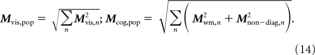
Single-neuron decomposition of population untangling dynamics in PRH. To determine the relationship between single-neuron response properties and population performance measures, we applied a method to parse each neuron's responses into intuitive signal modulation components, including firing rate modulations that could be attributed to: visual—changes in the visual image; working memory—changes in the identity of the target; diagonal—whether a condition was a target match or distractor; non-diagonal—other cognitive modulations (see Materials and Methods, Eqs. 7,8). We note that the method estimates and corrects for noise to ensure that trial-by-trial variability is not confused with signal. a, Plotted is the strength of each type of modulation (Eq. 8) as a function of time relative to stimulus onset, for three example neurons whose responses are dominated by one type of modulation. Also shown are the firing rate response matrices for each neuron, with spike counts averaged within the same window (0–140 ms after stimulus onset), each rescaled from the minimum (black) to maximum (white) firing rate. b, Left, The same plots depicted in a, but summed over all neurons in the PRH population. Right, The relationship between these signal modulation magnitudes and performances for the ideal observer and linear classifier can be described as a classifier component computed from the underlying signals followed by a mapping function that transforms the component values into performances. The classifier component for the linear classifier was computed from the diagonal signal alone. The classifier component for the ideal observer was computed by summing the linear classifier component signal with a second nonlinear classifier component that nonlinearly combined the visual and other cognitive signals (working memory and non-diagonal cognitive; see Materials and Methods, Eqs. 13–15). The same mapping function was used for both classifier predictions. c, Time courses for the actual (dotted, replotted from Fig. 3b, left) and estimated (solid) classifier performance values. d, Time courses of the linear, nonlinear, and summed classifier component signals. e, Time course for the actual (dotted, replotted from Fig. 3d) and estimated (solid, based on the data on the left) ratios of chance-corrected linear and nonlinear classifier components with the same conventions as Figure 3d, right. f, The mapping function used to convert classifier component magnitudes into performance predictions. The red and gray lines indicate the range of values used to estimate the linear and ideal observer, respectively. In b and d, the dotted box from 80 to 140 ms and the dashed line at 110 ms are provided as visual benchmarks.

Figure 7.

The hypothetical impact of IT modulation and code non-stationarities on PRH computation. a, A hypothetical illustration of how modulation non-stationarites in IT could impact computation in PRH. Two pairs of hypothetical IT cells (cells 1 and 2 vs 3 and 4) are shown, each of which contain one visual and one working memory neuron. Shown at the bottom are plots of the visual (black) and cognitive (red) modulation magnitudes as a function of time. Note that the two pairs are maximally activated at different times (e.g., 75 vs 135 ms). Thus, a model fit to extract diagonal signal at 135 ms (resulting in positive weights on neurons 3 and 4) will not generalize to produce diagonal signals at 75 ms. b, A hypothetical illustration of how code non-stationarities in IT could impact computation in PRH. Shown are one visual and one working memory neuron that combine to form a diagonal signal at 135 ms. Whereas the modulation magnitudes (i.e., the envelope of the combined visual and cognitive signals) of these hypothetical neurons are matched at 75 and 135 ms, the code (i.e., the response selectivity for the different visual and cognitive components) differs between these two time points, and thus a model fit at 135 ms will not generalize to produce diagonal signal at 75 ms. Visual and cognitive code components were computed by decomposing the response matrix at each time point via the linear basis (shown at the bottom; see Materials and Methods, Eq. 7).

A neuron's response matrix R can be decomposed into a weighted sum of these components:

where b_i indicates the ith component, and m_i indicates the weight (i.e., the amount of modulation) associated with the ith component. Components of the same type (i.e., the three visual components shown later in Fig. 7b) can then be grouped together to quantify the amount of each type of task-relevant modulation. More specifically, each type of modulation can be computed as the square root of the sum of the squared modulations along all relevant components:

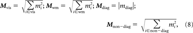where M_vis is the amount of visual modulation, M_wm is working memory modulation, M_diag is diagonal modulation, and M_non-diag is non-diagonal modulation.

Bias correction of response components.

When estimating the amount of modulation (or information) in a signal, noise and limited sample size are known to introduce a positive bias (Treves and Panzeri, 1995). For example, consider a hypothetical neuron that responds with the same average firing rate response to each of a set of stimuli. Because neurons are noisy, if we were to estimate these mean rates based on a limited number of repeated presentations, we would get the erroneous impression that the neuron does in fact differentiate between the stimuli. To overcome this problem, we estimated this bias using a bootstrap procedure and corrected for it. By reversing Equation 7, the estimated squared modulation along each component i is given by:

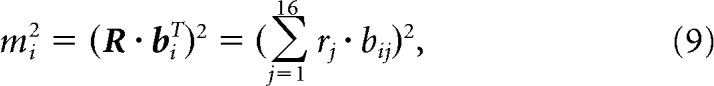where r_j indicates the neuron's average response to the jth condition, and b_ij indicates the jth entry of the ith basis component. To estimate the bias introduced by limited sampling, we applied a bootstrap procedure in which we first resampled with replacement 20 responses to each condition, and we then recomputed the squared modulation of these bootstrapped responses. The bias could be estimated by subtracting the modulation computed on the actual responses from the bootstrapped modulation (Efron and Tibshirani, 1994):

where m̂_i² indicates the squared modulation computed on the resampled responses. Bias was independently computed and subtracted from each type of modulation. Using procedures described in detail by Pagan and Rust (2014), we have confirmed the validity of this bias correction procedure and its equivalence to other bias correction approaches for this spike count window size, numbers of trials, and specific dataset.

Relationship between single-neuron responses and population performance.

The population performance of a linear classifier for discriminating target matches from distractors depends on the total amount of diagonal modulation (i.e., the differences in the firing rate responses to target matches compared with distractors). We define the total amount of diagonal modulation in a population M_diag,pop as the square root of the sum of the squared diagonal modulation M_diag,n for each neuron n:

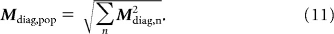To transform this measure into an estimate of the performance of a linear classifier, Perf_SVM, we applied the following formula (Poor, 1994; Averbeck and Lee, 2006):

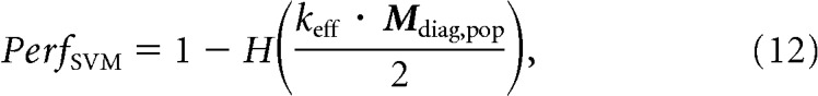where H is the complementary error function and k_eff is a classifier efficiency factor applied to account for the inability of the classifier to extract all the available information (for example, due to the limited amount of training data resulting in suboptimal choice of the parameters). This efficiency parameter is mathematically equivalent to the one introduced by Geisler and Albrecht (1997), although applied for a slightly different purpose in that case (to relate neural responses and behavior). We empirically estimated k_eff as 0.49 and we applied this same value for the estimation of both the linear classifier and the ideal observer (described below). We use the term “linear classifier component” to refer to the quantity k_eff · M_diag,pop.

The performance of an ideal observer for discriminating target matches from distractors can be approximated using the sum of the linear classifier component and a “nonlinear classifier component” k_eff · M_{NL–diag,pop} that reflects the amount of nonlinearly separable target match modulation contained in the combined visual and cognitive signals:

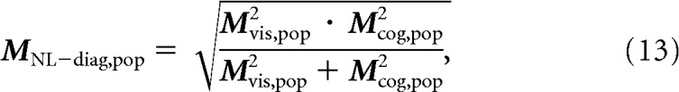where M_vis,pop is computed from each neuron's visual modulation analogously to M_diag,pop, and M_cog,pop measures the amount of cognitive modulation as the sum of working memory and non-diagonal modulation:

Finally, the performance of an ideal observer Perf_ID,OBS. can be estimated as:

Comparisons between estimated and actual performances for our recorded neurons are shown in Figures 4c and 5c, the magnitudes of linear and nonlinear classifier components are shown in Figure 4d, and the mapping function used to transform classifier components into estimated performances in Equations 12 and 15 is plotted in Figure 4e.

Figure 5.

Quantifying population performance and its single-neuron correlates in IT. a, The time course of ideal observer and linear classifier population performance in IT (solid line), and for comparison PRH (dotted line), plotted with the same conventions as Figure 3a. b, The time course of signal modulation components in IT (solid line) and, for comparison, PRH (dotted line), plotted with the same conventions as Figure 4b. c, A comparison of actual (dashed line) and estimated (solid line) ideal observer and linear classifier population performance for IT, plotted with the same conventions as Figure 4c. For both IT and PRH, populations included 164 neurons.

Fitting an instantaneous feedforward model of PRH to the IT responses

Our goal was to fit an instantaneous linear-nonlinear (LN) model to responses of IT neurons to determine whether this type of model could reproduce the dynamics observed in our recorded PRH population. To constrain the model, we assumed that the brain implements this transformation optimally and we thus determined the model parameters that maximized the total amount of diagonal modulation M_diag,pop in our model PRH. We always performed this maximization at a single time slice relative to stimulus onset, and we explored different positions of that training window (e.g., 75 vs 135 ms; Fig. 6b,c). Similar to the classification procedures described above, our model was designed to be cross-validated. On each iteration of the cross-validation procedure, 50% of the IT responses (10 repeats) were used to determine the LN model parameters, while the remaining 50% were passed through the instantaneous LN transformation to produce a set of “model PRH responses.” The model PRH responses were then compared with the actual PRH responses by measuring the performances of the same linear classifier and ideal observer described above (Fig. 6). The cross-validation of the model and the classifier was integrated, so that the same repeats used to train the model parameters were also used to train the classifier parameters, while the “test repeats” (i.e., the model PRH responses) were used to determine the classifier performances.

Figure 6.

A fixed, instantaneous model of PRH can reproduce the dynamics observed in PRH. An instantaneous linear-nonlinear model of PRH was fit to maximally untangle the responses of IT neurons. a, Three classes of neurons were created to produce the model PRH population. Shown are idealized depictions of one neuron from each class. For all three classes, the top of each plot (Input) depicts the hypothetical responses to the set of all target matches (red) and distractors (gray) in 2 dimensions of the 164 dimensional input population space; dotted lines represent the axis along which IT inputs are projected (i.e., the linear weights for one model neuron). Curved arrows point to the distributions of target matches and distractors following weighted linear combination. Below, the same distributions are shown as Output, following application of a nonlinearity (labeled). The first model neuron (left) inherited all of the linearly separable information available in IT; the linear weights for this neuron were determined as the optimal linear discriminant (i.e., the axis, represented by the dotted line, that maximizes the mean separation for the set of matches from the set of distractors) and the nonlinearity for this neuron consisted of exponentiation. The second class of neurons (2–15; center) computed linearly separable information; the weights for these neurons were determined as those that maximized the difference between the variances for target matches and distractors (see Materials and Methods) and the nonlinearities consisted of squaring. The final class of neurons (16–164; right) were not required to capture information at the time point used to train the model but were required to capture information at other times (see Materials and Methods). The linear weights for these neurons were determined as the set of axes that were orthogonal to the previously defined model neurons and those that were necessary to span the remaining IT space, and the nonlinearities for these neurons were exponential functions. b, c, Time course of ideal observer and linear classifier performance when model parameters were optimized for IT responses measured within a 25 ms time window centered at 75 ms (b) and 135 ms (c; yellow lines). Performance is shown for the following: the model (solid thick line), IT (dotted line), and PRH (solid thin line) for the ideal observer (gray) and linear classifier (red). The increase in linear classifier performance from IT to PRH is indicated as the shaded region, where light red indicates the increases reproduced by each model and darker red indicates the increases that remain unaccounted for; the overall magnitudes of increases that are accounted for are labeled. d, Signal types, shown with the same conventions as Figure 4b, for the following: the model shown in c (solid thick line), the actual IT data (dotted line), and the actual PRH data (solid thin line). The gray lines are provided as visual aids to compare the responses at 25 ms (dotted line), 75 ms (dashed line), and 135 ms (solid line) after stimulus onset.

Model structure.

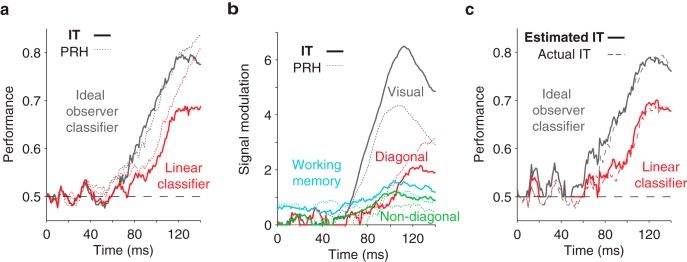
The responses of each model PRH neuron were created as an n-way linear combination of n IT responses, followed by a static nonlinearity, where n corresponds to the total number of neurons in our IT population (n = 164). The linear transformation was applied to individual trials (i.e., to the spike counts obtained for each of the conditions in one randomly selected repeat of the response matrix R_i for each ith IT cell) to produce a new matrix L:

where w_i indicates the weight applied to the ith IT neuron. The vectors of weights applied to create different PRH model neurons were constrained to be orthogonal and to have unitary norm:

where W_i and W_j are the vectors of weights for the ith and the jth model neurons. The matrix L resulting from Equation 16 was then passed through an instantaneous static nonlinearity to produce the model responses for the matrix on a single trial (described below). The trial-by-trial variability in the resulting model PRH thus arose from the trial-by-trial variability recorded in IT.

Fitting procedure.

The fitting procedure was designed to determine the linear weights for each model PRH neuron with the goal of maximizing the overall diagonal modulation in the model population. Maximizing diagonal modulation required us to generate model neurons via linear combinations of IT responses that both preserved the diagonal modulation already present in the input and extracted the maximal new diagonal signal (once nonlinearities were applied). We achieved this by splitting these two types of signals into two different classes of model neurons and, together, these two classes fully captured all the information available within the IT responses at the time point used to train the model (described in detail below). A third class of model neurons captured all remaining information present at all other time points (described below). This approach, which involved splitting the total amount of information into separate (linear and nonlinear) terms, is analogous to the linear and nonlinear classifiers with matched numbers of parameters introduced above.

To determine the parameters for the model, we began by normalizing the responses of each IT neuron on individual trials by subtracting the grand mean across all conditions and dividing the result by the SD across trials, pooled across all conditions. This normalization helped to ensure that the linear weights were assigned based on a measure that reflected the magnitude of responses as well as trial-by-trial variability (i.e., d′) as opposed to raw spike count responses alone. These “normalized responses” were used to find the linear weights, and once determined, the weights were converted back to units of spike count before the nonlinearities were applied; we note that the normalized responses were used only to fit the model parameters, whereas “un-normalized” spike counts were used to determine the cross-validated responses of the model itself.

The first model neuron was fit with the goal of preserving the diagonal signals contained in the recorded IT responses. This was achieved by choosing the linear weights for this neuron as the optimal linear discriminant between target match- and distractor-normalized responses (i.e., the vector of weights that connects the mean normalized response to target matches and the mean normalized response to distractors; Fig. 6a, left). The weights were then un-normalized, and the result of the linear combination with these weights L (computed according to Eq. 16) was centered (by subtracting the mean μ), and exponentiated to produce the final response matrix LN₁:

The monotonicity of the exponential function ensures that the rank-order of match and distractor responses is preserved, while at the same time making all responses positive.

The sets of linear weights for the second class of model PRH neurons were determined with the goal of maximizing the amount of diagonal modulation that could be extracted from the remaining IT population response space (i.e., after the axis defined by the weights of the first model neuron was removed, thus reducing the dimensionality by 1). The intuition behind the process used to extract diagonal information has been described in our previous report (Pagan et al., 2013), and is briefly summarized in Figure 6a, center. The key step that leads to diagonal modulation (i.e., separation between the mean normalized response to matches and the mean normalized response to distractors) involves choosing the linear weights that, once applied, maximize the differences between the variance for the target match-normalized responses and the variance for the distractor-normalized responses in the linearly transformed responses (e.g., a broad distribution in firing rates for target matches and a narrow distribution for distractors). These variance differences can then be translated into mean differences by a non-monotonic nonlinearity, such as a squaring operation (Fig. 6a, center). To find the weights that maximized the variance differences in the normalized responses to target matches and distractors, we designed a method similar in spirit to a PCA (which determines the dimensions with maximal variance). Whereas PCA directly computes the eigenvectors of the covariance matrix, we first computed the difference between the covariance matrices of the normalized responses to target matches and distractors and then applied the eigenvalue decomposition. The resulting set of eigenvectors thus defines the axes along which the variance differences between the normalized responses to target matches and distractors are maximal. Since our task has 16 conditions, the IT population response at a given time point has 15 degrees of freedom, i.e., 15 orthogonal axes with a significant amount of modulation of any kind. Because the first model PRH neuron described above captures 1 degree of freedom, the remaining variance differences are captured by the first 14 eigenvectors described above, and we use these to define the linear weights for the second class of neurons (after reversing the response normalization). To translate any variance differences produced into diagonal modulation, the resulting linear responses were centered (by subtracting the mean μ) and passed through a squaring nonlinearity (Adelson and Bergen, 1985) to produce the final response matrix LN₂:

Finally, the remaining 149 eigenvectors were used to define the linear weights for the third class of model PRH neurons (after reversing the response normalization). Although these axes are not required to capture information at the time point used to fit the model (see above), they are required to capture all the remaining information that exists within IT at different time points (Fig. 6a, right). These linear combinations were exponentiated (Eq. 18) to produce final response matrices.

Quantification of code non-stationarities

Code non-stationarities were defined as changes across time in a neuron's response modulations other than rescaling. In our analysis, we measured the degree of similarity of the responses at the reference time point of 135 ms and every other time point by computing Pearson's correlation coefficient. To determine the probability that differences arose from noise, we applied a split-half procedure. For each neuron, we began by determining the null distribution of correlations at the reference time point (135 ms) by bootstrapping the correlation across many random split-half draws across our set of repeated presentations. Next, we applied a similar procedure to compute the test distribution of correlations between the components at 135 ms and those at every other time point. The degree of non-stationarity was then measured via a nonparametric comparison between the null and the test distributions (see Fig. 8). More specifically, we computed the differences between randomly paired correlation values from the test and the bootstrap distributions, and we measured the p-value as the fraction of instances in which the correlation value across different time points was larger than the correlation value for split halves at 135 ms (Efron and Tibshirani, 1994).

Figure 8.

Visual and cognitive non-stationarities in IT. a, Quantification of the cognitive non-stationarities in our IT data. Center, Each row represents one neuron's cognitive non-stationarity as a function of time relative to stimulus onset; neurons are ranked by the peak time of their cognitive modulation. Brightness indicates the magnitude of cognitive modulation (i.e., the envelope of the combined cognitive signal for the 3 working memory and 8 non-diagonal cognitive components), relative to each neuron's peak, while hue indicates the degree of cognitive code non-stationarity (i.e., changes in the selectivity for different cognitive components) relative to the 135 ms time point, with stationary responses in yellow and non-stationarities in blue. Code components were computed at each time point as described in Figure 7b and Materials and Methods. The degree of code non-stationarity was measured by a noise-adjusted, cross-validated analysis which quantified the probability (the p-value) that changes in the code between two time points arose from noise (see Materials and Methods). Left, Plots of cognitive modulation as a function of time, normalized to range from 0 to 1, for four example neurons. Right, Plots of the largest 3 (of 11) cognitive code components as a function of time, for two example IT neurons. b, Visual non-stationarities, plotted using the same conventions as in a. In all plots, vertical lines are provided as visual aids to compare responses at 75 and 135 ms.

Pseudosimulation

A pseudosimulation approach was used to determine the contribution of each type of IT non-stationarity on the untangling dynamics of our PRH model. As an overview, we selectively manipulated different features of the noise-corrected IT modulations to make them stationary, regenerated Poisson trial-by-trial variability, reapplied our PRH model to the modified IT population, and quantified the delays between ideal observer classifier and linear classifier performance (see Fig. 9). Enforcing stationary responses was accomplished by modifying the structure of neural responses at each time point to resemble those at the reference time point of 135 ms, but rescaled such that the absolute amount of each signal type did not change. More specifically, we deconstructed the population response at each time point into three components: the total amounts of cognitive and visual modulation (i.e., the sum of modulations across the population), the pattern of modulations across neurons (i.e., the extent to which each neuron contributes to the overall modulation), and the code of each neuron's modulation (i.e., the selectivity for each component). In our pseudosimulations, we always maintained the total modulation computed at each time point. To measure the impact of modulation non-stationarites, we manipulated each neuron's components to match the code at 135 ms while leaving the modulation pattern intact. To measure the impact of code non-stationarities, we fixed the modulation pattern to match that at 135 ms while allowing the code components to change across time.

Figure 9.

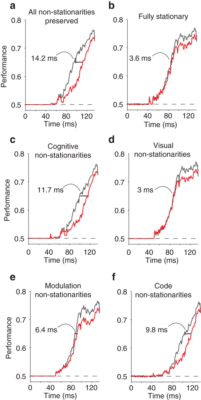
Impact of IT non-stationarities on the untangling dynamics of a model of PRH. To determine the effect that different types of IT non-stationarities might have on the dynamics of the target match representation in PRH, we performed a series of pseudosimulations in which we selectively imposed that one or more types of IT signals were perfectly stationary while leaving the others untouched, and we measured the delay that remained between ideal observer and linear classifier performances computed from the manipulated model PRH responses. a, The PRH model with no signal manipulation, but with Poisson trial-by-trial variability regenerated for IT (see Materials and Methods; compare with the actual data in Fig. 3). b, Manipulating all IT signals to become stationary nearly eliminates the delay in PRH. c–f, Contribution of the following types of IT non-stationarities to the delay observed in the PRH model, measured by making all other types of signals stationary: c, cognitive (both code and modulation), d, visual (both code and modulation), e, modulation (both visual and cognitive), and f, code (both visual and cognitive).

As a first step, the 15 bias-corrected modulation components for each neuron were computed for any given time point. Only the visual and cognitive (working memory and non-diagonal) components were manipulated. The total amounts of visual (M_vis,pop) and cognitive modulation (M_wm,pop and M_cog,pop, indicating working memory and the other cognitive components, respectively) were always preserved, and the components were normalized by dividing them by the total amount of modulation:

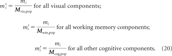The strength of the working memory components and that of the remaining cognitive components were computed separately to avoid mixing the actual working memory modulations present before the arrival of the visual signals from the spurious noise present at those early time points in the remaining modulation components.

To measure the effect of cognitive non-stationarities (see Fig. 9c), we preserved the normalized cognitive components measured in our data but replaced the normalized visual components with those measured at 135 ms, followed by rescaling to maintain the total visual modulation at that time point. Conversely, to measure the delay due to visual non-stationarities (see Fig. 9d), we preserved the normalized visual components but replaced the normalized cognitive components with those measured at 135 ms, followed by rescaling.

To manipulate the modulation non-stationarities in a manner that did not impact the code non-stationarities, we needed to quantify the fractional contribution of each neuron in the population to the overall modulation for each type of signal. We did this by separately summing the squared normalized visual components, the squared normalized working memory components for each neuron, and the remaining squared normalized cognitive components, thus resulting in three vectors expressing the relative contribution of each neuron to the total visual modulation and the total cognitive (working memory and remaining cognitive) modulation:

where v_vis,n represents the entry for the nth neuron in the vector expressing the relative contributions to total visual modulation, v_wm,n represents the entry for the nth neuron in the vector expressing the relative contributions to total working memory modulation, and v_cog,n represents the entry for the nth neuron in the vector expressing the relative contributions to total remaining cognitive modulation. Finally, dividing the normalized components by v_vis,n, v_wm,n, and v_cog,n, we obtained a set of “neuron-normalized” components whose values express each neuron's response preferences independent of each neuron's relative modulation:

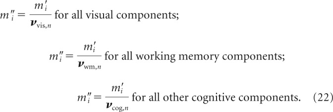To measure code non-stationarities (see Fig. 9f), we replaced the neuron-normalized components m″_i with those at 135 ms, followed by rescaling to maintain the total modulation at that time point. Conversely, to measure modulation non-stationarities (see Fig. 9e), we replaced the vectors v_vis, v_wm, and v_cog with those measured at 135 ms (while maintaining the neuron-normalized components m″_i), followed by rescaling.

Results

To explore the neural mechanisms involved in finding visual targets, macaque monkeys performed a well controlled yet simplified version of target search in the form of a delayed-match-to-sample task (Fig. 2a) as we recorded neural responses in IT and PRH. On each trial, monkeys sequentially viewed images and indicated when a target image appeared. We held the target fixed in short blocks of trials and we presented the same images as both targets and distractors in different blocks. Our experimental design included four images in all possible combinations as a visual stimulus (looking at), and as a target (looking for), resulting in 16 experimental conditions arranged in a four-by-four matrix (Fig. 2b). In these matrices, conditions with a fixed visual stimulus correspond to columns, and conditions with a fixed target (or working memory) correspond to rows. Additionally, the task required the monkeys to differentiate target match conditions, which fall along the diagonal of this matrix, from distractor conditions, which fall off the diagonal (Fig. 2b).

The “untangled” PRH target match representation is initially “tangled”

As described above, computing the solution to the monkeys' task (i.e., determining whether a currently viewed image is a target match or a distractor) requires combining visual and working memory information. In a recent paper (Pagan et al., 2013), we reported evidence that these signals combine within or before IT in the ventral visual pathway in a largely nonlinearly separable or “tangled” manner (i.e., one in which target match information is present but is not accessible to a linear population readout; Fig. 1, bottom right), followed by computations in PRH that reformat this information into a more linearly separable or “untangled” format (i.e., one more accessible to a linear population readout; Fig. 1, top right). This evidence was based in part on finding similar amounts of total target match information in IT and PRH, as measured by the performance of an ideal observer (see Materials and Methods, Eqs. 2–5), while also finding that a larger portion of this information was “linearly separable” (or untangled) in PRH compared with IT, as measured by the performance of a linear classifier applied to the same data (see Materials and Methods, Eq. 1). To gain deeper insight into the computations implemented by PRH to reformat nonlinearly separable target match signals arriving from IT, we investigated the temporal dynamics with which total and linearly separable signals evolved. We performed these analyses based on the spike count responses computed in 25 ms windows and we systematically shifted the positions of the windows relative to the onset of each visual image presented during our experiment. We found that total information arrived in PRH earlier than linearly separable information (Fig. 3a–c), consistent with target match information that initially arrived in PRH as partially tangled, followed by the arrival of more untangled target match information after a short delay.

Quantifying the magnitude of the delay, or equivalently, the differences in the latencies with which total versus linearly separable target match information arrived in PRH, required us to set a performance criterion to compute latency (e.g., the time required for performance to reach 0.65). We computed latencies for a range of such criteria (see Materials and Methods, Eq. 6). We found that the latency differences between total and linearly separable information were fairly constant across the broad range of performance criteria for which we were able to determine them (range, 0.55–0.775; latency difference range, 9.3–12.9 ms; mean latency difference = 11.7 ms; Fig. 3b, left) and that these latency differences were significant (e.g., p = 0.011 for a criterion of 0.65 and p < 0.05 for all criteria 0.6–0.775). Although the latencies of linearly separable signals computed in this manner were longer than those for nonlinearly separable signals, linearly separable signals were also slightly smaller in their overall magnitude (Fig. 3b, left, yellow). To determine the degree to which these magnitude differences produced the latency differences we were observing, we selected the subset of our data in which performance of the linear classifier and ideal observer was matched on average in a window placed at 135–140 ms, and we recomputed latencies for the same trials at earlier time points (see Materials and Methods). Average latency differences were similar, albeit slightly smaller, for magnitude-matched data (mean delay across all criteria was 11.2 ms for the magnitude-matched data compared with 11.7 ms for the original data) and magnitude-matched latency differences remained significant across a broad range of criteria (e.g., p = 0.018 at a criterion of 0.65; p < 0.05 for criterion 0.6–0.775; Fig. 3b, right). The delay in the arrival of linearly separable compared with total information was confirmed in each monkey individually (e.g., for a criterion of 0.65, monkey 1: delay = 15.4 ms, p = 0.031; monkey 2: delay = 12.2 ms, p = 0.034; data not shown; for magnitude-matched data, monkey 1: delay = 13.9 ms, p = 0.046; monkey 2 delay = 10.9 ms, p = 0.048; Fig. 3c).

One possible interpretation of these results is that the format of target match information in PRH changes over time from a more nonlinearly separable to a more linearly separable format. However, the analyses described above were performed using two readout approaches (i.e., an SVM linear classifier and an ideal observer nonlinear classifier) that, while relatively common, differ in their numbers of parameters and how the parameters are optimized. These differences may confound the interpretation of our results, particularly given that, above, we indirectly infer the amount of nonlinearly separable information at each point in time by comparing “total” and “linear” performance as opposed to measuring it directly. As a control analysis, we developed two new classifiers to measure linear and nonlinear information directly, and in a comparable manner, including matched numbers of parameters. Our approach is analogous to a polynomial expansion in that it seeks to deconstruct the classifier decision boundary into a set of terms of increasing order (e.g., w₁ * x + w₂ * x²…). To equate the numbers of linear and nonlinear parameters, the linear classifier was characterized by parameters associated with the first-order term (i.e., the means of the firing rate distributions) and the nonlinear classifier was characterized by parameters associated with the second-order term (i.e., the variances of the firing rate distributions; see Materials and Methods). A comparison of the temporal evolution of performance for this linear and this nonlinear classifier (Fig. 3d, left) revealed that at early times (e.g., 80 ms), linear and nonlinear performance were approximately matched, but at later times (e.g., 110 ms), nonlinear performance began to plateau as linear performance continued to rise. Consequently, chance-corrected linear classifier performance grew to over threefold nonlinear performance by 140 ms (Fig. 3d, right). These results are consistent with a target match representation that arrives in PRH as partially tangled (i.e., an approximately balanced combination of nonlinear and linear target match information) and then becomes more untangled (i.e., more linearly separable). These results are inconsistent with the alternative proposal that target match information increases in its overall amount but does not change its format with time.

What types of single-neuron responses account for population untangling dynamics?

The population-based framework described above is useful for understanding the combined PRH population representation. As a complementary analysis, we were interested in relating these descriptions of population dynamics with more intuitive descriptions of the signals reflected in the responses of individual neurons. As an overview of how we determined this relationship, we applied a technique to parse each neuron's responses into intuitive components (i.e., the magnitudes of visual and different types of cognitive modulation) and we derived the relationships between these single-neuron modulations and population performance for the ideal observer and linear classifiers. Our decompositions assume that population performance is not impacted by correlated trial-by-trial variability between neurons (“noise correlations”), which we have previously determined to be true in our data (Pagan et al., 2013).

To deconstruct the firing rate modulations of each neuron into intuitive components, we applied a noise-corrected, ANOVA-like analysis (see Materials and Methods, Eqs. 7–9) to parse each neuron's responses into firing rate modulations that could be attributed to the following: changing the visual image (visual; Fig. 2b); changing the identity of the target (working memory; Fig. 2b); changing whether a condition was a target match or a distractor (diagonal; Fig. 2b); and changes between other non-diagonal cognitive conditions (e.g., looking at image 2 and for image 4 versus for image 3; Fig. 2b). Figure 4a shows the decomposition for three example neurons and Figure 4b shows the total magnitudes of these signals across the PRH population as a function of time. We found that the visual signal was the strongest type of signal in PRH, followed by the diagonal, working memory, and non-diagonal signals, respectively. Consistent with weak “persistent activity,” working memory signals were present before the other signals, which followed a stimulus-evoked time course.

Next, we determined the relationship between the magnitudes of these signals and the predicted population performance for both readouts as a two-stage process in which signals were first combined into “classifier components” which were then converted to performance values via a mapping function (Fig. 4b; see Materials and Methods, Eqs. 11,12). We imposed that the mapping function be matched for the two types of classifiers (i.e., the complementary error function; see Materials and Methods) but allowed the two classifiers to rely on different signals. We found that the evolution of linear classifier performance was well described by the amount of diagonal signal alone (i.e., the “linear component”; Fig. 4c,d, red). In contrast, we found that accounting for the evolution of ideal observer performance required summing the linear component with a “nonlinear component” term that nonlinearly combined the visual signal and the other two types of cognitive signals (working memory plus non-diagonal cognitive; Fig. 4d, cyan; see Materials and Methods, Eqs. 13–15). This result can be understood in the context that performance of the ideal observer depends upon the degree to which the responses to the same images presented as target matches and distractors are nonoverlapping (Fig. 1), and any type of cognitive modulation (diagonal, working memory, or non-diagonal cognitive) will be at least partially effective at producing this separation. Notably, the temporal dynamics of the linear and nonlinear classifier components inferred from these underlying signals provided a reasonable match to direct measures of the same quantities, including the saturation of the nonlinear component at ∼110 ms as the linear component continued to rise (compare Fig. 4d, left with Fig. 3d), leading to an increasing ratio between linear and nonlinear dynamics as a function of time (Fig. 4d, right). This correspondence allowed us to pinpoint the source of the population dynamics in PRH. We found that the saturation of the nonlinear classifier component could largely be attributed to a visual signal that peaked at ∼110 ms and then began to fall (Fig. 4b, gray, d, cyan, dashed line). In contrast, the linear classifier component continued to rise beyond 110 ms due to a continually rising underlying diagonal signal (Fig. 4b,d, dashed line). Consequently, the representation of target match signals initially arrived in PRH in a more tangled format because visual and working memory signals initially arrive in PRH to some degree as separate signals (coinciding with an initial wave of diagonal signal), followed by the emergence of a more untangled target match representation ∼10–15 ms later, when diagonal signals become stronger and visual information decreases.

Dynamic representation in PRH can be accounted for by instantaneous PRH computation

The dynamics underlying untangling in PRH could provide an important constraint on descriptions of how this computation is implemented, and thus we were interested in determining the classes of models that could account for the delay between nonlinearly separable and linearly separable target match information in PRH. Following from our previous results (Pagan et al., 2013), we can begin by ruling out simple descriptions in which these delays are entirely inherited from the primary input to PRH—IT—because IT contains less linearly separable information. As illustrated in Figure 5, a–c, the linearly separable target match information (and corresponding diagonal signals) that do exist in IT are delayed relative to total information (and other types of signals), but they are smaller in magnitude than those in PRH. Thus, although the delays between the arrival of tangled versus untangled information in PRH are likely inherited in part from IT, they cannot fully account for the result.

In our previous report, we presented evidence that a simple, feedforward model could account for the transformation of other types of IT signals into diagonal signals in PRH (Pagan et al., 2013). In that model, computation in PRH was instantaneous (and spike count windows were broad). Thus, upon finding that target match signals evolved dynamically in PRH, we naturally assumed that accounting for these dynamics would require us to extend our model to incorporate dynamic PRH computation (e.g., as a result of implementing these computations in complex, recurrent circuits). We were very surprised to discover that instead of attributing these delays to PRH, they could be accounted for by a variant of a feedforward model in which PRH computations were fixed and acted instantaneously—but crucially—upon input from IT that changed its content over time (as described below).

To evaluate this class of model, we considered whether a model fit to our recorded IT responses could produce a model population that reproduced the dynamics we observed in PRH. To constrain the fits, we assumed that computations in PRH sought to transform the maximal amount of nonlinearly separable (i.e., tangled) information arriving from IT into a linearly separable (i.e., untangled) format. Fitting an instantaneous, feedforward model of PRH computation that maximally extracted diagonal signal from our recorded IT responses required us to develop novel model-fitting procedures. The novel model-fitting procedures we describe here incorporate non-trivial extensions to ones we have previously reported (Pagan et al., 2013).

As an overview, the responses of each model PRH neuron were computed via an LN model as a weighted combination of all IT neurons, followed by an instantaneous nonlinearity. The input to the model consisted of the responses of 164 IT neurons to the 16 experimental conditions and the output of the model consisted of 164 model PRH responses to those same conditions. Model responses were determined for individual trials (i.e., trial-by-trial variability in our model PRH was inherited from the recorded IT responses) and the model was fully cross-validated, meaning that we used 50% of our data to train the model (10 repeats for each condition) and we assessed model performance using the other half of our data (the other 10 repeats). As described in more detail below, we fit the model to the IT responses at a single time point (e.g., 135 ms) and these parameters were held fixed for all the other time points. We emphasize that the model fits are confined to the data recorded from IT and our goal is to evaluate the degree to which these model response properties are similar to our recorded PRH data.

Linearly separable target match information amounts to a difference in the average responses across the set of target matches compared with the set of distractors (Fig. 6a, red vs gray). To understand how the model converted nonlinearly separable target match information into a linearly separable format (i.e., increased mean differences), it is useful to consider the model PRH neurons as three classes (Fig. 6a). First, a single-model PRH neuron served to combine and inherit all of the linearly separable information that already existed in IT (Fig. 6a, left). We determined the linear weights for this neuron (i.e., the weights to apply to each IT input neuron before summation) as the optimal linear target match/distractor discriminant (see Materials and Methods). The responses for this neuron were then computed by applying an exponential nonlinearity (e.g., a “soft threshold;” Pillow et al., 2008) to the linearly weighted IT responses. The second class of model PRH neurons “computed” linearly separable information from the inputs arriving from IT. We determined the weights for these model neurons using an insight from our previous work (Pagan et al., 2013), in which we established that the crucial property that needs to be maximized through linear weighting is the difference between the variance across the responses to target matches and distractors in the linearly combined responses (i.e., a high variance for the responses to one set and a low variance for the other; Fig. 6a, center). Under appropriate conditions, these variance differences are transformed into mean differences via a non-monotonic (i.e., a squaring) nonlinearity. We determined the linear weights for these neurons using a method similar to PCA (i.e., an eigenvector decomposition of the difference of the covariance matrices for matches and distractors; see Materials and Methods). The number of these neurons was set as the number required to capture all the available information at the training time point, given the number of degrees of freedom in our experiment (see Materials and Methods). The final class of model PRH neurons served to capture any remaining information at different time points (see Materials and Methods).

As described above, the goal of our model was to transform the maximal amount of nonlinearly separable (i.e., tangled) information arriving from IT into a linearly separable (i.e., untangled) format within the class of models we were working with (i.e., the n-wise LN model). Because the representation arriving from IT changes its content with time (as elaborated below), this required us to select a specific time window for the optimization. To do so, we began by making the reasonable assumption that connectivity between IT and PRH was established for this task during the experience of looking for targets, and we thus looked to the learning literature to guide our selections. We selected the width of our spike count window, 25 ms, to fall within the range of integration times over which synaptic plasticity is thought to occur (Froemke and Dan, 2002). We then explored different positions for this window relative to stimulus onset. Training windows placed shortly after total information arrives in PRH, at 75 ms, produced linearly separable target match information without a delay relative to the arrival of total information, but only increased linear classifier performance by a small amount (i.e., this model accounted for 35% of the performance increases observed in PRH over IT; Fig. 6b). This was because the parameters that were optimal for these early time windows failed to generalize to later time points where the IT representation differs (described in more detail below). Training windows placed later, at 135 ms, produced larger overall increases in linearly separable information (i.e., this model accounted for 86% of the increases observed in PRH over IT; Fig. 6c). However, this information was delayed relative to the arrival of total information. This is because the parameters appropriate for extracting linearly separable information at these later times failed to generalize to earlier times. These results suggest that processing speed and information content trade off one another in PRH due to the dynamic nature of input arriving from IT.

Strikingly, the model PRH produced by training at the later time point of 135 ms had many response properties similar to the actual PRH. Most notably, the magnitude of the delay between the arrival of total and linearly separable information was similar between the model and the actual PRH (for a criterion of 0.65, actual PRH = 11.9 ms, model = 13.8 ms; Fig. 6c). The model also approximately reproduced many other notable and subtle properties of the actual PRH responses that were also not directly fit during the optimization. These include the approximate amounts and time courses of the increases in diagonal modulation from IT to PRH (Fig. 6d, red), the decreases in visual modulation from IT to PRH (Fig. 6d, gray), and the existence of the working memory modulation before the stimulus-evoked response (persistent activity; Fig. 6d, cyan). We note that slightly lower overall ideal observer and linear classifier performance in the model compared with the actual PRH (Fig. 6c, red and gray solid thick versus thin lines) is partially imposed by slightly lower ideal observer performance in the input to the model, IT (Fig. 6c, gray dotted line) coupled with the constraint that the model cannot artificially create information.

We emphasize that in our model, delays in the arrival of linearly separable relative to total target match information result in large part from computations that are implemented in PRH instantaneously (i.e., without a delay). How could this be possible? Our model works as follows. Shortly after the onset of a test stimulus (∼25 ms; Fig. 6d, gray dotted line), visual signals have not yet arrived in IT and working memory signals exist in isolation; these working memory signals are passed on to PRH. Because computing the target match signal requires both visual and cognitive signals, total target match information is absent in both IT and PRH at this time. Sometime later (∼75 ms; Fig. 6d, gray dashed line), stimulus-evoked visual signals arrive in IT, which in turn passes both visual and cognitive information to PRH, and total target match information is present in both areas. However, little diagonal signal is created in PRH because the specific contents of the visual and cognitive inputs arriving from IT are misaligned with the biophysical parameters of the PRH neurons (i.e., the synaptic weights), which have been optimized to produce diagonal signals at a later time. Consequently, little untangled target match information exists in PRH. As time passes (∼135 ms; Fig. 6d, gray solid), the specific content of the IT representation becomes aligned to the fixed PRH biophysical parameters (as elaborated below), and diagonal signals are created, thus producing a more linearly separable, untangled target match representation in PRH.

The IT representation exhibits many different types of non-stationarities

The results presented above suggest that the delays between the arrival of total and linearly separable target match information in PRH must somehow arise from computations performed on an input representation from IT that changes its content over time (i.e., is non-stationary) and thus we wished to better understand the specific types of non-stationarities that existed in IT. One useful, albeit broad, definition of “non-stationarity” is any change in the neural population response other than an overall rescaling. In fact, if the IT modulations were simply rescaled at different points in time (i.e., relative to 135 ms), our model of PRH would not exhibit delays between total and linearly separable information (as shown later in Fig. 9b). More narrowly, non-stationarities can arise from two conceptually distinct factors. First, non-stationarities can arise from changes in the distribution of information across the neural population over time (“modulation non-stationarities”). For example, information can be carried by different subsets of neurons at different times, due to variability in the response latencies across a population. Consequently, the synaptic strengths appropriate for creating an untangled target match signal at one time point can fail to generalize to other time points in which different IT neurons carry information (Fig. 7a). Second, non-stationarities can arise from changes in the selectivity of individual neurons for the specific components that combine to form the overall modulation envelope (“code non-stationarities”). Similar to the potential impact of modulation non-stationarities, the potential impact of code non-stationarities is an inability to generalize the biophysical parameters that are appropriate for creating an untangled target match signal at one time point to different points in time (Fig. 7b).

Measuring code non-stationarities for different types of signals (e.g., visual vs cognitive) required us to develop a way to measure the rank-order selectivity for different visual versus cognitive components of the signal at different points in time. We note that this cannot be achieved by simply measuring the rank-order selectivity preferences for the 16 different experimental conditions because each condition is a combination of both visual and cognitive information (i.e., a combination of the current visual stimulus and the current target). To parse these signals, we developed a method to linearly transform each neuron's 16 entry response matrix into 16 different “component” responses where 3 of the components describe the visual response, 3 components describe the working memory response, 1 component describes the diagonal response, 8 components describe the non-diagonal cognitive responses, and a final component corresponds to the neuron's grand mean firing rate (Fig. 7b, bottom; see Materials and Methods, Eqs. 7, 8). Together, these components form an orthonormal basis and, thus, this procedure is similar to a PCA, but instead of finding the stimulus dimensions that account for the most variance, we assign the dimensions a priori to capture intuitive, task-relevant components of a neuron's response, and determine the amount of firing rate modulation along each dimension (see Materials and Methods, Eqs. 8, 9). Notably, the different components combine to form the signal modulation envelopes depicted in Figure 4, a and b (e.g., the 3 visual components combine to determine the visual signal modulation envelope; see Materials and Methods, Eq. 8).

Figure 8 includes a visualization of IT component and code non-stationarities (similar to that by Brincat and Connor, 2006) analyzed separately for the cognitive (Fig. 8a) and visual (Fig. 8b) signals. In these plots, rows correspond to the responses of individual neurons, plotted as a function of time relative to stimulus onset. The modulation envelope for each neuron is depicted by brightness (black to bright), and neurons are ranked by the times at which the peaks of their envelopes fell. Modulation non-stationarities are thus indicated by changes in the brightness patterns between two columns of the plot. As illustrated by the considerable change in the subpopulations of neurons that were active at (e.g.) 75 versus 135 ms (orange lines), modulation non-stationarities were present in both the visual and cognitive signals in IT. This can also be seen by examining the modulation envelopes for four example neurons with a variety of latencies and peak response times (Fig. 8a,b, left).

In contrast, the degree of code non-stationarity for each neuron (relative to 135 ms) is indicated in these plots by color, with stationary responses indicated in yellow and non-stationarities indicated in blue. To measure code non-stationarities, we compared each neuron's selectivities for the different components at 135 ms with its selectivities at every other time point, and we determined the probability (the p-value) that changes in selectivity were due to trial-by-trial variability (see Materials and Methods). As illustrated by the presence of blue in these plots (Fig. 8a,b, center), code non-stationarities were present in both the cognitive and the visual signals. Example neurons with visual and cognitive codes that were both stationary and non-stationary are shown (Fig. 8a,b, right).

Code non-stationarities in IT are the largest contributors to PRH model dynamics

The analysis presented above suggests that many different types of non-stationarities exist in IT (i.e., modulation and code non-stationarities for both visual and cognitive signals); to what degree did the dynamics of our PRH model depend on each type? To evaluate this question, we performed a series of pseudosimulations in which we manipulated our recorded IT responses such that one or more types of signals were artificially made stationary, and we quantified the delays that remained between total and linearly separable information in our model of PRH. For example, to quantify delays due to modulation non-stationarities, we manipulated the data such that the selectivity to code components for all neurons was perfectly stationary relative to the 135 ms time point used to train the model, while preserving any modulation non-stationarities that existed in the data (see Materials and Methods, Eqs. 20–22). Similarly, to quantify the delays due to code non-stationarities, we enforced the modulation signals to be perfectly stationary by adjusting the relative contribution of each neuron (i.e., the magnitude of the envelope for each type of modulation) at every time slice to match the 135 ms reference time slice, while preserving any code non-stationarities that existed in the data (see Materials and Methods, Eqs. 20–22). Notably, the impact of both types of pseudosimulation was confined to the format of the signal components (by changing their distribution across neurons or the code selectivity within individual neurons), and never modified the total amount of any type of signal modulation across the population at any time slice. The results of these simulations revealed that many different types of non-stationarities contribute to the delays between the arrival of total and linearly separable information in our model of PRH, with the cognitive and code non-stationarities being the largest contributors (Fig. 9). The fact that visual non-stationarities exist in IT (Fig. 8b) but do not provide a sizable contribution to the delays we observe in our model (Fig. 9d) can be explained by the fact that ideal observer performance relies on a combination of visual and cognitive signals (Eqs. 13–15), and because cognitive signals are smaller, their non-stationarities play a larger role (e.g., they serve as a “bottleneck” for model computation).

Discussion

One of the biggest challenges in studying a high-level brain area like PRH is parsing the response properties that have been “inherited” from its inputs from those response properties that are “computed” at that stage, and our findings demonstrate that these determinations need to be made carefully. Here we illustrate that the target match signals found in PRH are well described as arising from computations implemented in PRH that act on inputs arriving from IT. Somewhat counterintuitively, these signals evolve dynamically within PRH but can be accounted for by instantaneous PRH computation. This is because the inputs from IT change their content over time, and thus the biophysical parameters (e.g., synaptic weights) that are optimal for extracting diagonal signals at a time that maximizes information content (i.e., 135 ms following stimulus onset) fail to generalize to earlier times where the IT representation differs (e.g., 75 ms).

If changes in the IT target match representation over time were simply due to rescaling (i.e., gradual increases in signal modulation magnitudes produced by stimulus-evoked responses), our model of PRH would fail to reproduce the dynamics that we observe in our PRH data (Fig. 9b). Rather, we find that our recorded IT responses reflect multiple types of non-stationarities that combine to produce dynamic computation in PRH (Fig. 9c–f). The types of non-stationarities we describe are not exotic. Specifically, the “modulation” non-stationarity that we describe arises in large part from a diversity of latencies across the IT population, and this type of latency diversity has been documented in many different visual brain areas (Schmolesky et al., 1998). Similarly, neurons that do not simply rescale their response selectivity as a function of time following stimulus onset are also well documented, particularly in IT (Eskandar et al., 1992; Chelazzi et al., 1993; Sugase et al., 1999). What our results demonstrate is that these commonly observed response dynamics can produce seemingly dynamic computation downstream; or conversely, that observing the dynamic evolution of a signal at one stage of processing should not immediately be attributed to delays in the mechanisms used to compute it (e.g., its implementation in complex, recurrent circuits).

To establish our main effect—a delay between the arrival of total versus linearly separable information in PRH—we compare the performances of two types of readout rules applied to the data collected from PRH (i.e., an ideal observer and an SVM linear classifier; Fig. 3a–c). We also compare the performances of a linear and a nonlinear classifier with matched structure and number of parameters (Fig. 3d), and these two classifiers are very similar to our model of PRH computation (i.e., here we envision computation in PRH as a nonlinear readout of IT; Fig. 6). This classification scheme—which is analogous to the first two terms of a polynomial expansion of the optimal classifier boundary—is related to others that have previously been proposed, but it does not directly correspond to any that we are aware of. In particular, although other classification methods (e.g., quadratic discriminant analysis and quadratic kernel SVM) also rely on covariance differences to compute a decision boundary, they are not explicitly formulated in terms of an LN cascade of operations, whereas our method specifies an intermediate population of biologically plausible LN units, upon which a linear readout could be applied. Notably, when we apply classifiers to the data collected from PRH (Fig. 3), we apply them in a manner that might be regarded as a “dynamic” readout (i.e., we allow the parameters to vary between time bins), whereas when we use these classifiers as models of PRH computation (Fig. 6), we enforce that the readout be “static” (i.e., we fit the parameters at a specific time slice). Our rationale behind this is that we were interested in evaluating the hypothesis that signals in PRH could be described as arising from a static computation, and thus we began by quantifying signals in PRH in the absence of making this assumption, and we then compared these results with a model of PRH when this assumption was enforced. Stated differently, here we first present the classifier analyses merely as quantification tools (Fig. 3), and then we proceed to evaluate one as a model of PRH computation (Fig. 6).

It is also worth noting that our model is “functional” and, similar to other functional models (Adelson and Bergen, 1985; Rust et al., 2006), it is designed to capture neural computation in an interpretable manner. To clearly describe how PRH might compute linearly separable information arriving from IT, our model separates those signals from the ones that are inherited from IT by parsing them into different model PRH neurons (Fig. 6a). We note that it is highly unlikely that the brain separates signals in the same way. Rather, the responses of actual PRH neurons likely reflect a combination of both inherited and computed linearly separable target match signals using mixtures of the mechanisms used in our model for different “classes” of neurons.

In developing our model of PRH, we assumed that the task-relevant connections between IT and PRH were learned, and we used this assumption to guide our selections of the spike count window width (25 ms) and its placement (135 ms following stimulus onset). How reasonable are these assumptions? Although little is known about the specific mechanisms that regulate synaptic plasticity in PRH during complex cognitive tasks, neural plasticity during reinforcement learning is thought to be largely regulated by dopaminergic inputs (for review, see Schultz, 2007), and we know that PRH contains high densities of both dopamine-carrying fibers and dopamine receptors (for review, see Richmond, 2006). Consistent with a specific training window, some have hypothesized that a phasic dopamine response could serve to “switch on” learning at a precise time following stimulus onset (Redgrave and Gurney, 2006; Redgrave et al., 2008). Thus, although much remains to be discovered about synaptic plasticity in PRH, our assumptions are consistent with our current understanding of those mechanisms.

In agreement with earlier reports (Eskandar et al., 1992; Chelazzi et al., 1993, 1998), our results suggest that during visual target search tasks, the IT representation is non-stationary; how do these non-stationarities arise in IT? Possibly from multiple sources. First, visual non-stationarities have been reported previously in IT under conditions of passive viewing (Sugase et al., 1999), suggesting that cognitive (i.e., working memory) signals are not the only contributors. Second, IT non-stationarities may be produced via the mechanisms that combine visual and working memory information within or before IT in the ventral visual pathway. A series of studies documented non-stationarities within V4, IT, and PRH as monkeys performed a target search task in which they had to find targets among sets of multiple stimuli (Chelazzi et al., 1993, 1998, 2001). The authors proposed that target-specific working memory signals may exert their influence via a top-down bias to IT (and/or V4) neurons, followed by competitive interactions within IT that enhance the responses to target stimuli and suppress the response to distractors (Desimone and Duncan, 1995). Finally, cognitive non-stationarities may be “inherited” from prefrontal cortex where the persistent, working memory representations of target identity are thought to be housed (Miller et al., 1996), but individual prefrontal neurons are reported to respond only transiently during some fraction of the memory period (Brody et al., 2003; Machens et al., 2010). As our results demonstrate, regardless of their source, non-stationarities in IT have important consequences for downstream computation.

Finally, we note that our report includes a number of methodological advancements in data analysis and model fitting that may be useful for other studies. First, we apply a method to quantify the amounts of different types of task-relevant signals contained within heterogeneous and difficult to understand brain areas like IT and PRH (Figs. 4, 5; elaborated in the work by Pagan and Rust, 2014). In our study, this provided an important constraint for our model PRH (Fig. 6) and allowed us to quantify multiple types of non-stationarities in IT (Figs. 8, 9). Second, we introduce derivations that connect these single-neuron measures with population-based analyses (Fig. 4c). This allowed us to determine the underlying neural signal dynamics that gave rise to dynamics in the population-based classifier performance measures (Fig. 4b,c). Finally, we introduce a means of “leapfrogging” over a considerable amount of neural processing that we do not understand to determine the computations performed in a high-level brain area (i.e., determining computation in PRH in the absence of a model of processing up to and including IT). We achieved this by fitting an LN model to our recorded IT responses to produce a model PRH that we compared with our PRH data (Fig. 6). Whereas our previous attempts at fitting such models were constrained to brute-force searches of simple (pairwise) LN combinations, here we used an insight from our previous work (Pagan et al., 2013) to fit a more realistic model in which larger numbers of IT neurons combine to form the responses of neurons in PRH.

References

- Adelson EH, Bergen JR. Spatiotemporal energy models for the perception of motion. J Opt Soc Am A. 1985;2:284–299. doi: 10.1364/JOSAA.2.000284. [DOI] [PubMed] [Google Scholar]
- Averbeck BB, Lee D. Effects of noise correlations on information encoding and decoding. J Neurophysiol. 2006;95:3633–3644. doi: 10.1152/jn.00919.2005. [DOI] [PubMed] [Google Scholar]
- Bichot NP, Rossi AF, Desimone R. Parallel and serial neural mechanisms for visual search in macaque area V4. Science. 2005;308:529–534. doi: 10.1126/science.1109676. [DOI] [PubMed] [Google Scholar]
- Brincat SL, Connor CE. Dynamic shape synthesis in posterior inferotemporal cortex. Neuron. 2006;49:17–24. doi: 10.1016/j.neuron.2005.11.026. [DOI] [PubMed] [Google Scholar]
- Brody CD, Hernández A, Zainos A, Romo R. Timing and neural encoding of somatosensory parametric working memory in macaque prefrontal cortex. Cereb Cortex. 2003;13:1196–1207. doi: 10.1093/cercor/bhg100. [DOI] [PubMed] [Google Scholar]
- Chelazzi L, Miller EK, Duncan J, Desimone R. A neural basis for visual search in inferior temporal cortex. Nature. 1993;363:345–347. doi: 10.1038/363345a0. [DOI] [PubMed] [Google Scholar]
- Chelazzi L, Duncan J, Miller EK, Desimone R. Responses of neurons in inferior temporal cortex during memory-guided visual search. J Neurophysiol. 1998;80:2918–2940. doi: 10.1152/jn.1998.80.6.2918. [DOI] [PubMed] [Google Scholar]
- Chelazzi L, Miller EK, Duncan J, Desimone R. Responses of neurons in macaque area V4 during memory-guided visual search. Cereb Cortex. 2001;11:761–772. doi: 10.1093/cercor/11.8.761. [DOI] [PubMed] [Google Scholar]
- Churchland MM, Yu BM, Cunningham JP, Sugrue LP, Cohen MR, Corrado GS, Newsome WT, Clark AM, Hosseini P, Scott BB, Bradley DC, Smith MA, Kohn A, Movshon JA, Armstrong KM, Moore T, Chang SW, Snyder LH, Lisberger SG, Priebe NJ, et al. Stimulus onset quenches neural variability: a widespread cortical phenomenon. Nat Neurosci. 2010;13:369–378. doi: 10.1038/nn.2501. [DOI] [PMC free article] [PubMed] [Google Scholar]
- Desimone R, Duncan J. Neural mechanisms of selective visual-attention. Annu Rev Neurosci. 1995;18:193–222. doi: 10.1146/annurev.ne.18.030195.001205. [DOI] [PubMed] [Google Scholar]
- Efron B, Tibshirani RJ. An introduction to the bootstrap. Boca Raton: CRC; 1994. [Google Scholar]
- Eskandar EN, Richmond BJ, Optican LM. Role of inferior temporal neurons in visual memory. 1. Temporal encoding of information about visual images, recalled images, and behavioral context. J Neurophysiol. 1992;68:1277–1295. doi: 10.1152/jn.1992.68.4.1277. [DOI] [PubMed] [Google Scholar]
- Froemke RC, Dan Y. Spike-timing-dependent synaptic modification induced by natural spike trains. Nature. 2002;416:433–438. doi: 10.1038/416433a. [DOI] [PubMed] [Google Scholar]
- Geisler WS, Albrecht DG. Visual cortex neurons in monkeys and cats: detection, discrimination, and identification. Vis Neurosci. 1997;14:897–919. doi: 10.1017/S0952523800011627. [DOI] [PubMed] [Google Scholar]
- Gibson JR, Maunsell JHR. Sensory modality specificity of neural activity related to memory in visual cortex. J Neurophysiol. 1997;78:1263–1275. doi: 10.1152/jn.1997.78.3.1263. [DOI] [PubMed] [Google Scholar]
- Haenny PE, Maunsell JHR, Schiller PH. State dependent activity in monkey visual-cortex. 2. Retinal and extraretinal factors in V4. Exp Brain Res. 1988;69:245–259. doi: 10.1007/BF00247570. [DOI] [PubMed] [Google Scholar]
- Liu Z, Richmond BJ. Response differences in monkey TE and perirhinal cortex: stimulus association related to reward schedules. J Neurophysiol. 2000;83:1677–1692. doi: 10.1152/jn.2000.83.3.1677. [DOI] [PubMed] [Google Scholar]
- Machens CK, Romo R, Brody CD. Functional, but not anatomical, separation of ”what” and ”when” in prefrontal cortex. J Neurosci. 2010;30:350–360. doi: 10.1523/JNEUROSCI.3276-09.2010. [DOI] [PMC free article] [PubMed] [Google Scholar]
- Maunsell JHR, Sclar G, Nealey TA, DePriest DD. Extraretinal representations in area-V4 in the macaque monkey. Vis Neurosci. 1991;7:561–573. doi: 10.1017/S095252380001035X. [DOI] [PubMed] [Google Scholar]
- Miller EK, Desimone R. Parallel neuronal mechanisms for short-term-memory. Science. 1994;263:520–522. doi: 10.1126/science.8290960. [DOI] [PubMed] [Google Scholar]
- Miller EK, Erickson CA, Desimone R. Neural mechanisms of visual working memory in prefrontal cortex of the macaque. J Neurosci. 1996;16:5154–5167. doi: 10.1523/JNEUROSCI.16-16-05154.1996. [DOI] [PMC free article] [PubMed] [Google Scholar]
- Pack CC, Born RT. Temporal dynamics of a neural solution to the aperture problem in visual area MT of macaque brain. Nature. 2001;409:1040–1042. doi: 10.1038/35059085. [DOI] [PubMed] [Google Scholar]
- Pagan M, Rust NC. Quantifying the signals contained in heterogeneous neural responses and determining their relationships with task performance. J Neurophysiol. 2014 doi: 10.1152/jn.00260.2014. in press. [DOI] [PMC free article] [PubMed] [Google Scholar]
- Pagan M, Urban LS, Wohl MP, Rust NC. Signals in inferotemporal cortex and perirhinal cortex suggest an untangling of visual target information. Nat Neurosci. 2013;16:1132–1139. doi: 10.1038/nn.3433. [DOI] [PMC free article] [PubMed] [Google Scholar]
- Pillow JW, Shlens J, Paninski L, Sher A, Litke AM, Chichilnisky EJ, Simoncelli EP. Spatio-temporal correlations and visual signalling in a complete neuronal population. Nature. 2008;454:995–999. doi: 10.1038/nature07140. [DOI] [PMC free article] [PubMed] [Google Scholar]
- Poor HV. An introduction to signal detection and estimation. New York: Springer; 1994. [Google Scholar]
- Redgrave P, Gurney K. The short-latency dopamine signal: a role in discovering novel actions? Nat Rev Neurosci. 2006;7:967–975. doi: 10.1038/nrn2022. [DOI] [PubMed] [Google Scholar]
- Redgrave P, Gurney K, Reynolds J. What is reinforced by phasic dopamine signals? Brain Res Rev. 2008;58:322–339. doi: 10.1016/j.brainresrev.2007.10.007. [DOI] [PubMed] [Google Scholar]
- Richmond BJ. Dopamine-dependent associative learning of workload-predicting cues in the temporal lobe of the monkey. In: Pinaud R, Tremere LA, De Weerd P, editors. Plasticity in the visual system: from genes to circuits. New York: Springer; 2006. pp. 309–320. [Google Scholar]
- Rust NC, DiCarlo JJ. Selectivity and tolerance (“invariance”) both increase as visual information propagates from cortical area V4 to IT. J Neurosci. 2010;30:12978–12995. doi: 10.1523/JNEUROSCI.0179-10.2010. [DOI] [PMC free article] [PubMed] [Google Scholar]
- Rust NC, Schultz SR, Movshon JA. A reciprocal relationship between reliability and responsiveness in developing visual cortical neurons. J Neurosci. 2002;22:10519–10523. doi: 10.1523/JNEUROSCI.22-24-10519.2002. [DOI] [PMC free article] [PubMed] [Google Scholar]
- Rust NC, Mante V, Simoncelli EP, Movshon JA. How MT cells analyze the motion of visual patterns. Nat Neurosci. 2006;9:1421–1431. doi: 10.1038/nn1786. [DOI] [PubMed] [Google Scholar]
- Schmolesky MT, Wang Y, Hanes DP, Thompson KG, Leutgeb S, Schall JD, Leventhal AG. Signal timing across the macaque visual system. J Neurophysiol. 1998;79:3272–3278. doi: 10.1152/jn.1998.79.6.3272. [DOI] [PubMed] [Google Scholar]
- Schultz W. Behavioral dopamine signals. Trends Neurosci. 2007;30:203–210. doi: 10.1016/j.tins.2007.03.007. [DOI] [PubMed] [Google Scholar]
- Smith MA, Majaj NJ, Movshon JA. Dynamics of motion signaling by neurons in macaque area MT. Nat Neurosci. 2005;8:220–228. doi: 10.1038/nn1382. [DOI] [PubMed] [Google Scholar]
- Sugase Y, Yamane S, Ueno S, Kawano K. Global and fine information coded by single neurons in the temporal visual cortex. Nature. 1999;400:869–873. doi: 10.1038/23703. [DOI] [PubMed] [Google Scholar]
- Treves A, Panzeri S. The upward bias in measures of information derived from limited data samples. Neural Comput. 1995;7:399–407. doi: 10.1162/neco.1995.7.2.399. [DOI] [Google Scholar]