

Abstract
Vehicle emissions represent one of the most important air pollution sources in most urban areas, and elevated concentrations of pollutants found near major roads have been associated with many adverse health impacts. To understand these impacts, exposure estimates should reflect the spatial and temporal patterns observed for traffic-related air pollutants. This paper evaluates the spatial resolution and zonal systems required to estimate accurately intraurban and near-road exposures of traffic-related air pollutants. The analyses use the detailed information assembled for a large (800 km2) area centered on Detroit, Michigan, USA. Concentrations of nitrogen oxides (NOx) due to vehicle emissions were estimated using hourly traffic volumes and speeds on 9,700 links representing all but minor roads in the city, the MOVES2010 emission model, the RLINE dispersion model, local meteorological data, a temporal resolution of 1 hr, and spatial resolution as low as 10 m. Model estimates were joined with the corresponding shape files to estimate residential exposures for 700,000 individuals at property parcel, census block, census tract, and ZIP code levels. We evaluate joining methods, the spatial resolution needed to meet specific error criteria, and the extent of exposure misclassification. To portray traffic-related air pollutant exposure, raster or inverse distance-weighted interpolations are superior to nearest neighbor approaches, and interpolations between receptors and points of interest should not exceed about 40 m near major roads, and 100 m at larger distances. For census tracts and ZIP codes, average exposures are overestimated since few individuals live very near major roads, the range of concentrations is compressed, most exposures are misclassified, and high concentrations near roads are entirely omitted. While smaller zones improve performance considerably, even block-level data can misclassify many individuals. To estimate exposures and impacts of traffic-related pollutants accurately, data should be geocoded or estimated at the most-resolved spatial level; census tract and larger zones have little if any ability to represent intraurban variation in traffic-related air pollutant concentrations. These results are based on one of the most comprehensive intraurban modeling studies in the literature and results are robust. Recommendations address the value of dispersion models to portray spatial and temporal variation of air pollutants in epidemiology and other studies; techniques to improve accuracy and reduce the computational burden in urban scale modeling; the necessary spatial resolution for health surveillance, demographic, and pollution data; and the consequences of low resolution data in terms of exposure misclassification.
Keywords: Air pollution, Exposure, Exposure misclassification, Traffic
1 Introduction
The transport sector is the largest emitter of nitrogen oxides (NOx) and carbon monoxide (CO), and mobile sources are major sources of other pollutants, including particulate matter (PM2.5) and volatile organic compounds (VOCs). (European Environment Agency 2013, U.S. Environmental Protection Agency 2013) Traffic-related air pollutants are emitted at or near ground level and mostly in urban areas where they can cause locally-elevated concentrations that have been associated with adverse health effects, e.g., exacerbation of asthma, impaired lung function, cardiovascular morbidity and mortality, adverse birth outcomes, and cognitive declines. (U.S. Environmental Protection Agency 2008, Health Effects Institute 2010, Laumbach and Kipen 2012) Exposure to traffic-related pollutants is widespread, occurring in numerous locations, e.g., residences, workplaces, schools, and playgrounds located near high traffic roads. Health impacts can be significant at local to global scales. (Huang and Batterman 2000, Wu and Batterman 2006) Low income and minority individuals often live near high traffic roads, and these populations are particularly vulnerable. (Tian, Xue et al. 2013) Recognizing the importance of these effects and the many people potentially affected, the number of scientific and policy investigations on traffic-related air pollutants has grown rapidly. Such investigations are conducted at project, intraurban, multicity, national and international levels, and for purposes that include exposure and risk estimation, epidemiology, health impact assessment, accountability and regulatory compliance. (Molitor, Jerrett et al. 2007, Isakov, Touma et al. 2009, Health Effects Institute 2010, Bell, Morgenstern et al. 2011, Hystad, Setton et al. 2011, Lobdell, Isakov et al. 2011)
Exposure to traffic-related air pollutants occurs in “on-road,” ”near-field” and “far-field” micro-environments. (Batterman 2013) On-road exposure applies to commuters, pedestrians, cyclists and workers such as police and truck drivers, who travel and work on high traffic roads, and to pedestrians, cyclists and runners. This applies to many individuals, e.g., in the US, an estimated 119 million persons commute using cars, trucks and vans, 7 million use public transportation, 4 million walk, and 0.75 million cycle, and the average one-way commute lasts 25 min (McKenzie and Melanie 2011). The second and most widely analyzed microenvironment is the region lying within several hundred meters of major roads. Many people live, work, go to school and recreate in this near-field microenvironment, e.g., 18% of US homes are within 300 feet of a four-lane highway, railroad or airport; this increases to 22 and 25% for Hispanic and Black households, respectively. (U.S. Department of Housing and Urban Development and U.S. Department of Commerce 2011) The far-field environment applies to areas more distant from major roads and urban areas where traffic-related emissions become part of the “urban plume.” At this scale, spatial and temporal gradients are present but blurred.
Concentrations of traffic-related air pollutants show dramatic temporal and spatial variation in on-road and near-field environments. For example, PM2.5, ultrafine PM (currently unregulated), volatile organic compounds (VOCs), NO, and polycyclic aromatic hydrocarbons (PAHs) demonstrate steep gradients in concentrations, attaining elevated levels near and on roads, and a return to background levels at distances of roughly 150 to 200 (Barzyk, George et al. 2009, Hagler, Baldauf et al. 2009, Hu, Fruin et al. 2009, Karner, Eisinger et al. 2010). This variation leads to significant uncertainty in quantifying concentrations and exposures. (Health Effects Institute 2010) For example, due to their limited number and siting criteria, (Wilson, Kingham et al. 2005, Hystad, Setton et al. 2011) data from central ambient monitoring sites capture little of this variability. While additional information will be provided by the new near-road monitoring network for certain pollutants (e.g., NO2) measured within 50 m of high traffic roads in the US, this network is not designed to provide spatial coverage or to estimate population exposures. (Batterman 2013) It is important to reduce the spatial and temporal errors in concentration estimates used to estimate exposures in epidemiology, health impact and environmental justice studies. (Jerrett, Arain et al. 2005, Brauer 2010, Sheppard, Burnett et al. 2012) Such errors have deleterious effects, e.g., exposure misclassification can diminish the effect sizes and bias results towards the null (no-effect) in epidemiology studies, incorrectly predict risks in health impact studies, and misidentify affected populations in justice studies.
The challenge of estimating exposures of traffic-related air pollutants has been tackled by a variety of methods, e.g., simple proximity assessments, statistical land-use regression models, source-oriented models incorporating mechanistic sub-models (for emissions, dispersion, transformation, exposure), and hybrid approaches combining several approaches. (Huang and Batterman 2000, Sharma and Khare 2001, Jerrett, Arain et al. 2005, Wilson, Kingham et al. 2005, Hoek, Beelen et al. 2008, Lipfert and Wyzga 2008, Brauer 2010, Health Effects Institute 2010) To estimate exposures and health impacts, exposure estimates are being applied to census and other geocoded data. The use of such data with geographical information systems (GIS) has become routine, and potentially can inform policies at local to national scales. (English, Neutra et al. 1999, Lin and Lin 2002, Jin and Fu 2005) With a few exceptions, e.g., certain air pollution epidemiology studies and a small number of quantitative health impact studies, estimates of health impacts attributable to traffic-related air pollutants have used simplified large-scale box-type models that do not represent spatial gradients or short-term fluctuations in concentrations. (Apte, Bombrun et al. 2012, Chart-asa, Sexton et al. 2013) Refined and validated methods are needed to estimate exposures and better understand the burden of disease attributable to traffic-related air pollutants, and to identify susceptible populations. Indeed, the modeling system described below was developed to support an epidemiological investigation of effects of diesel exhaust emissions on the respiratory health of children. (Vette, Burke et al. 2013)
1.1 Objectives
This paper evaluates spatial resolution issues involved in estimating near-field exposures of traffic-related air pollutants for epidemiological, health risk and policy applications. The analysis uses a large-scale and detailed case study centered on Detroit, Michigan, USA, a city that contains many neighborhoods bisected by major roads with heavy truck traffic, to estimate hourly to annual average concentrations at spatial scales as fine as 10 m. Model estimates are compared with standards and monitoring data. We evaluate several interpolation (joining) approaches, determine the spatial resolution requirements, and estimate exposure misclassification associated with common zonal units. Study limitations are discussed, and recommendations are made regarding modeling and exposure assessment practices for urban scale applications.
2 Methods
2.1 Emissions inventory and dispersion modeling
A detailed, link-based NOx emission inventory for roads in Detroit and surrounding Wayne County was compiled for the year 2010. NOx was selected as an air pollutant representative of emissions from traffic. (Health Effects Institute 2010, European Environment Agency 2013) The road network included the location, link type as described by its National Functional Classification (NFC), the annual average daily traffic (AADT), and the average vehicle speed for each of 9,701 road links (Figure 1). These links include all but local neighborhood streets and alleys. AADT and speed were derived using road counts and travel demand modeling (TDM) with link-specific inputs. Hourly traffic volume, fleet mix, and speed were estimated for each link and allocated into 8 vehicle classes, representing motorcycles, light-duty gasoline vehicles, light-duty diesel vehicles, light-duty gasoline trucks with gross vehicle weight (GVW) less than 6001 pounds, light-duty gasoline trucks with GWV>6001 pounds, light-duty diesel trucks, heavy-duty diesel trucks, heavy-duty gas vehicles, and heavy-duty diesel vehicles. Hourly emissions were estimated using emission factors from MOVES2010a (http://www.epa.gov/otaq/models/moves/) for primary exhaust emissions adjusted for the 2010 Detroit vehicle age distribution, thus producing an hourly, link-based emissions inventory that accounted for traffic activity.
Figure 1.
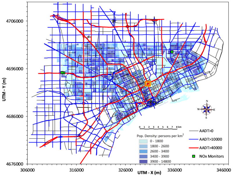
Modeled road network for Detroit. Blue shaded areas shows city of Detroit and population density. Orange rectangle is region for high (10 m) resolution analysis. Locations of the three NOx monitoring sites are indicated.
Pollutant concentrations were predicted using RLINE (http://www.cmascenter.org/r-line/), a research grade dispersion model for near-roadway assessments under development by US EPA. This steady-state plume-dispersion model incorporates newly developed algorithms for predicting concentrations from road sources, including at receptors near roads. (Snyder, Venkatram et al. 2013, Venkatram, Snyder et al. 2013) Hourly meteorological data were taken from Detroit City airport, which was determined to be representative of the study area, and processed by AERMET. Modeling used several sets of receptors. The first used extremely fine resolution to model a high impact area, the 175/194 intersection, and consisted of 12,221 receptors over a 1.0 × 1.2 km grid on 10 m centers. The second set used the same resolution to estimate concentrations at three area NOx monitoring sites (121 receptors, 100 × 100 m area). The third modeled the entire Detroit area using 27,622 receptors over a 34.5 × 23.0 km grid on 150 m centers. In all cases, the modeled road network extended well beyond the receptor network.
Estimating concentrations with high spatial resolution at the urban scale is computationally intensive. The Supplemental Materials describe techniques used to speed up calculations, and present additional details on the emissions inventory and dispersion modeling.
2.2 Concentration errors due to spatial resolution
Errors in estimating concentrations at different spatial resolutions were estimated as the difference between “known” and estimated (or interpolated) concentrations. Unlike the joining methods discussed later that compute area averages, this evaluation is concerned with concentrations at discrete points. Model estimates were taken as the known concentrations, calculated using a dense receptor grid (10 m spacing). At locations where concentrations were assumed to be unavailable, NOx concentrations were interpolated using modeled concentrations at locations 10, 20, 40, 80 or 160 m distant (Δx). Note that a receptor grid with 20 m spacing allows any (arbitrary) location to be within ∼10 m from a receptor where the concentration is known.
Concentrations were estimated using the “nearest neighbor” (NN) technique and the inverse-distance-weighted (IDW) average. Errors for the two types of interpolations were determined as both absolute and relative differences (RΔC, %) between known (predicted) and interpolated concentrations between all pairs of receptors separated by distance Δx. The RΔC is equivalent to the absolute fractional bias. At finer spatial resolutions, i.e., as Δx → 0, both errors approach 0. (Interpolations and error calculations are detailed in the Supplemental Materials.)
A comprehensive approach was taken to estimate errors: we examined the most important averaging times, all time periods, all receptor pairs, and Δx = 10, 20, 40, 80, and 160 m. To portray the variation of the results, the distribution of error metrics was computed. Two criteria were established: keeping ΔC below 25 μg/m3 (25% of the annual NO2 National Ambient Air Quality Standard (NAAQS) of 100 μg/m3), and keeping RΔC% below 25%. These criteria balance practicality and precision. Because concentration gradients become steep near major roads, errors were stratified by proximity to roads. These analyses used the receptor grid for the I75/I94 junction and all pairs of receptors, thus sample sizes were large, e.g., 11,781 receptor pairs for Δx=10 m and 6,141 pairs for Δx=160 m for IDW interpolations, and twice that for NN estimates since both E-W and N-S directions were considered.
2.3 GIS and population analysis
Concentrations from the third set of receptors (27,622 receptors on 150 m centers over Detroit) were assigned to the four zonal systems commonly used at the intra-urban scale: ZIP code, census tract, census block, and property parcel. Digital boundaries for the first three zones were obtained from the TIGER-Line database; shape files for property parcels were obtained from DataDrivenDetroit [http://datadrivendetroit.org/]. Each parcel's population was estimated by assigning it to a single census block, using a point-in-polygon spatial join between parcel centroids and block polygons, and distributing the population of each block evenly among its parcels. The study area included 386,068 parcels. To analyze the geographic zones using the same area and population, the 12 ZIP codes on the boundary of the study area that did not fully overlap the parcel data were excluded, which included the cities of Hamtramck and Highland Park (embedded in central northern Detroit). The final analysis considered 357,962 parcels, 12,238 blocks, 287 tracts and 25 ZIP codes, representing a population of 0.67 million, and 93% of the Detroit population.
Both vector- and raster-based GIS methods were used to join values from model receptors to the four zonal units. With the exception of the vector-based approach for parcels, these methods approximate areal average concentrations, which provide satisfactory estimates of pollution exposure assuming a uniform distribution of the population within the zone. (Brindley, Wise et al. 2005) The vector-based approach retained the point and polygon forms of receptors and zones, and overlaid the point map of concentration values (i.e., receptor data) with the geographic zones using the spatial join tool in ArcGIS 10.2. For the three larger zones (block, tract, ZIP code), the point-in-polygon method (Okabe and Sadahiro 1997) was used to assign concentration values to the zone (polygon) that contained it completely, and the zone concentration was estimated as the average of all associated points. For census blocks, the 150-m receptor spacing resulted in 8,774 (40%) blocks without associated points; these were assigned the concentration of the nearest receptor. Parcel-level data was handled by joining each parcel to the single receptor closest to the boundary of the parcel.
The raster-based approach mapped both receptors and zones to rasters. Zone polygons were converted to a high-resolution 3-m raster for which each cell's value was uniquely assigned to a single zone (parcel, block, tract or ZIP code). Three concentration rasters were created: (1) a simple up-scaling of a 150 m grid created from receptor points to 3 m resolution in which each 3 m cell was assigned the same value as the 150 m cell containing it; (2) an IDW average using the nearest 12 receptors, and (3) a regularized spline interpolation using 12 receptors and a 0.1 weighting. This gave three sets of concentration estimates, all calculated using the zonal statistics tool in the spatial analyst extension of ArcGIS 10.2 (ESRI, Redlands, CA, USA).
Exposure misclassification due to the zonal aggregations was calculated using several approaches. First, concentrations were visualized using maps that showed concentrations, roads and zone boundaries. Second, distributions and descriptive statistics compared exposure (population-weighted) concentrations at five scales (ZIP code, block group, block, track, receptor). Third, statistics were derived for the deviation (residual) of the exposure estimate, defined as the difference between concentrations in the larger units (e.g., ZIP code) and that for the corresponding parcel(s), weighted by population with the assumption that concentrations at the parcel level, the smallest available with population data, were correct. Fourth, correlations and scatter plots compared the various exposure measures. Finally, concentrations for each zone were grouped into quintiles, and contingency tables were used to evaluate misclassification.
3 Results
3.1 Aggregate emissions and estimated NOx levels
The modeled road network for Detroit (Figure 1) included 9,701 links and a total road length of 3,064 km. NOx emissions totaled 14,715 t/yr (product of the emission rate and link length summed across all links and all hours of the year). Most emissions occur on principal arterials (30.4%); other freeways (26.1%), interstates (19.9%), and minor arterials (15.2%). Light duty gas vehicles, followed by heavy-duty diesel vehicles, emit the bulk of NOX emissions.
Figure 2 depicts very high resolution (10 m grid) concentrations at the I75/I94 intersection (inset square in Figure 1) for four scenarios: the monthly average, which is representative of long-term levels; the highest 24-hr average at each receptor (which is not simultaneous in time); the 98th percentile 1-hr average (also not simultaneous); and the 24-hr average for Jan. 19, a day when winds arose from only the west quadrant. The averaging period and time of interest depend on the application, e.g., the highest 1- and 24-hr maps show areas (“hotspots”) affected by high but short-term concentrations, relevant for acute health effects, e.g., asthma exacerbation and some cardiovascular effects; monthly and annual averages are appropriate for chronic effects. Concentrations are dominated by emissions from the large highways. For the 175/194 area, monthly average NOx concentrations range from 8 to 190 μg/m3 (median=24 μg/m3), and 98th percentile 1-hr concentrations from 34 to 780 μg/m3 (median=101 μg/m3). The spatial patterns shift considerably on daily and hourly levels, showing either higher or lower levels and greater asymmetry with respect to roads.
Figure 2.
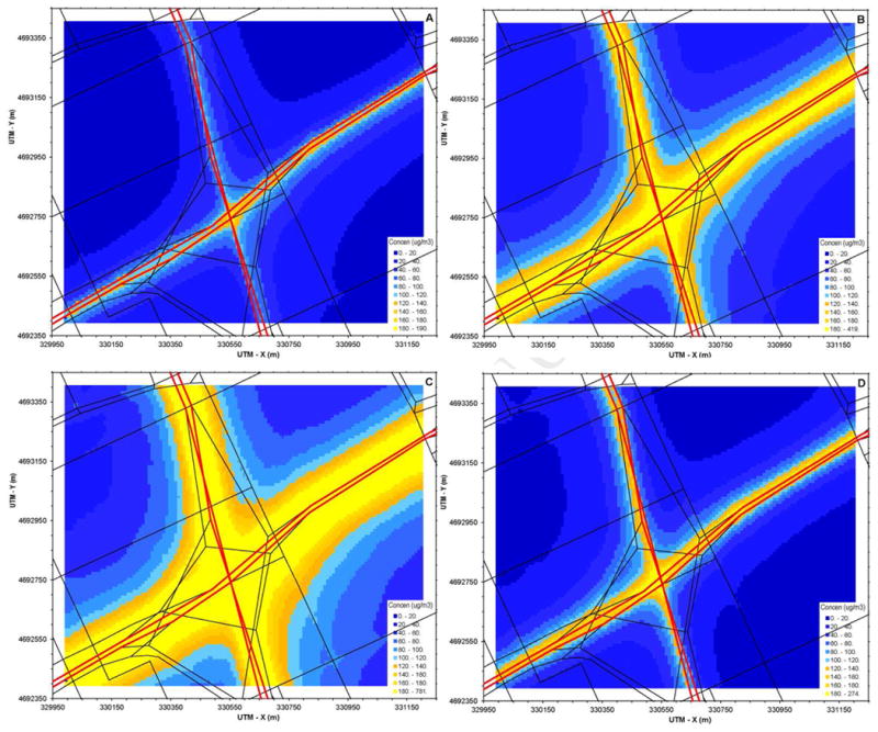
NOx concentrations in μg/m3 around the I75/I94 junction for four scenarios: (a) monthly average; (b) maximum 24-hr average; (c) 98th percentile 1-hr average, and (d) 24-hr average for Jan. 19, 2010. I75 runs roughly N-S; I94 runs SW-NE. Concentration scale shown in inset. Receptor grid uses 10 m spacing over a 1.0 ×1.2 km area.
Predicted concentrations are not directly comparable to the NO2 NAAQS (100 μg/m3 on an annual average basis, 185 μg/m3 on a 1-hr 98th percentile basis, averaged over 3 years) because NOx (not NO2) was estimated, only primary traffic-related emissions were considered, and modeling guidelines for compliance determinations were not followed (e.g., a non-regulatory model was used). NO2/NOx ratios observed at area monitoring sites (described below) ranged from 0.4 (near highway) to 0.8 (distant from highway). Using the 98th percentile 1-hr prediction (780 μg/m3) and the near-road ratio of 0.4, the estimated 1-hr concentration is 312 μg/m3. This concentration occurs at an on-road location (intersection of I75 and I94) where no monitoring data are available. Such calculations suggest the significance of vehicle emissions; further analysis is needed to evaluate the possibility of exceeding the NAAQS.
Model results are compared to ambient monitoring data collected in Detroit. As in most cities, available monitoring sites provide little if any spatial resolution. Long term trends are available at a single monitoring site (East Seven Mile, E7M) located in a residential neighborhood, downwind from the urban core and 3.5 km from freeways. Recently, two near-road monitoring sites were commissioned in Detroit, Eliza Howell 1 and 2 (EH1, EH2) sites located 10 and 100 m north of I96 and just west of Detroit city limits, but within the modeling domain. (Figure 1 shows site locations.) At this location, I96 has an AADT of 150,000 vehicles per day. These sites have good coverage for 2012 (86-96% completeness, depending on site). Monitored annual average NOx concentrations are 30, 81 and 37 μg/m3 at E7M, EH1 and EH2 sites, respectively; 98th percentile 24-hr concentrations are 99, 200 and 125 μg/m3; and 98th percentile 1-hr concentrations are 155, 261 and 158 μg/m3. Trends at E7M show that annual averages decreased by 3% since 2010; 98th percentile 1-hr concentrations increased by about 3%. Predicted NOx concentrations from roadway emissions at receptors representing E7M, EH1 and EH2 locations are 3, 52 and 19 μg/m3 on an annual basis, respectively; 6, 136 and 56 μg/m3 for 24-hr highest concentrations; and 9, 225 and 81 μg/m3 for 98th percentile 1-hr concentrations. As expected, estimated levels fall below the monitoring data since contributions from area, point and background sources are not included. However, the higher concentrations, estimated during periods when local sources would dominate impacts, are consistent with observations, particularly at the near-road sites. Spatial gradients around the monitoring sites, investigated using 10 m receptor grids around each monitor, show EH1 predictions were sensitive to position, a result of its proximity to the roadway, e.g., moving the receptor 10 m closer increased annual levels by 18%; moving it 10 m further from the road dropped levels by 14%. EH2 and especially E7M monitoring sites showed much lower sensitivity. While the available data do not permit a full model evaluation, this analysis suggests that the near-road estimates of traffic-related NOx concentrations are reasonable.
3.2 Concentration errors and spatial resolution
The effect of spatial resolution on concentration estimates is first evaluated using the 10 m grid centered around the I75/I94 junction and the maximum 24-hr NOx average (Figure 2B). Concentration differences for NN and IDW interpolations increase substantially as interpolation distance Δx increases. For example, the NN interpolations for Δx=10 m yield median and 95th percentile errors of 2.1 and 26 μg/m3, respectively; comparable values for Δx=160 m are 55 and 167 μg/m3 (Figure 3A). As expected, IDW interpolations perform better, e.g., interpolations for Δx=10 m have median and 95th percentile errors of only 0.2 and 9.0 μg/m3, respectively, and 31 and 141 μg/m3 for Δx=160 m (Figure 3B). The performance of IDW interpolations is particularly favorable for distances below 40 to 80 m, and for all but the highest percentile errors, which occur very near major roads (discussed below). While absolute errors depend on the averaging time, e.g., errors are smaller for monthly averages since concentrations are lower, Figures 3A and B properly depict trends. However, scaling issues motivate the relative measures (shown as Figures 3C and 3D for NN and IDW joining methods). Considering the better-performing IDW method, relative errors remain below 25% for 99.6% of estimates for Δx=10 m, 99% for Δx=20 m, 98% for Δx=40 m, 78% for Δx=80 m, and 35% for Δx=160 m. Again, these results apply to the specific scenario modeled (i.e., the highest 24-hr concentration). However, results for each 24-hr average in January (n=31) gave very similar performance, e.g., 98±1=1, 96±2, 88±3, 68±4 and 32±7% (average±standard deviation) of estimates met the 25% criterion for Δx=10, 20, 40, 80 and 160 m, respectively. As another test, each daily 1 -hr maximum was tested, with nearly identical results (only the standard deviation increased slightly due to greater day-to-day variation.) These results are robust as they reflect a wide range of meteorological conditions and concentration statistics, although the results pertain to the specific area modeled. They also suggest that relative errors are broadly applicable and insensitive to averaging time and concentration statistic.
Figure 3.
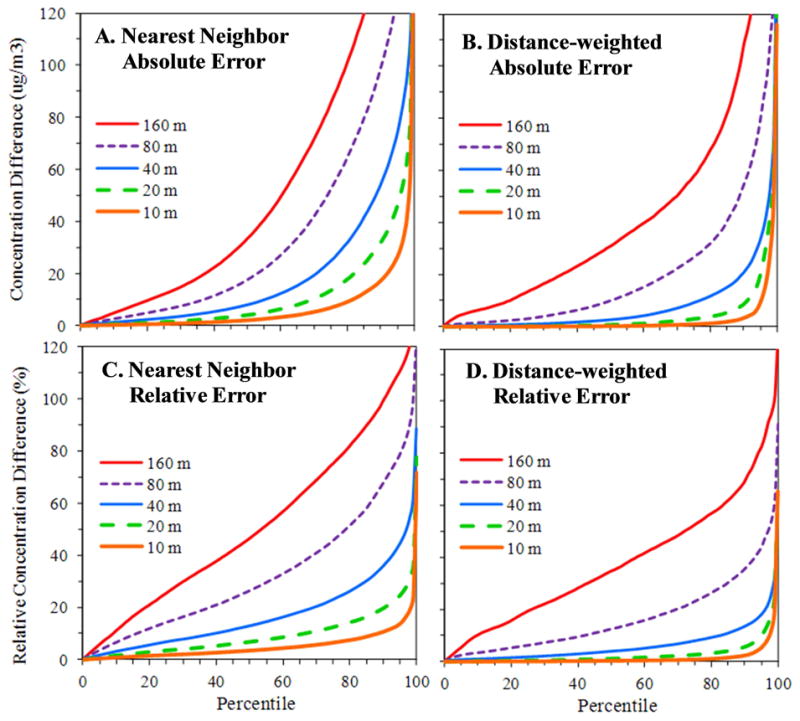
Distribution of error measures for highest 24-hr average and estimates from 10 to 160 m from known values. Absolute concentration differences (ΔC) for (A) nearest-neighbor and (B) inverse-distance-weighted estimates. Relative concentration differences (RΔC) for (C) nearest-neighbor and (D) inverse distance-weighted estimates.
To display the effect of location, Figure 4A stratifies relative errors by the distance to larger roads (AADT>30,000), and highlights larger (95th percentile) errors. For all interpolation distances Δx, relative errors are highest near major roads where gradients are sharpest. Figure 4B shows the fraction of receptors attaining a criterion of relative errors below 25%, again stratified by the distance to large roads. For Δx=10 to 40 m, nearly all receptors meet the criterion at any distance. For Δx=80 to 160 m, however, few receptors within 20 m of roads meet the criterion, although few individuals likely live this close to centerlines of interstate highways. At distances of exceeding 60 m, Δx=80 m interpolations perform well, and as do 160 m interpolations at distances of 80 to 100 or more. (Again, the spatial resolution needed is equivalent to about 2 Δx.) These results use IDW interpolations and all 24-hr averages in January (n=31), and thus are robust. (Supplemental Figures 1 and 2 show additional analyses stratifying by distance.)
Figure 4.

Distance stratified analysis of relative errors (concentration differences or RΔC) for inverse-distance weighted estimates and estimates from 10 to 160 m from known values. A. 95th percentile errors. B. Percentage of receptors meeting 25% relative error criterion at given distance.
Three GIS methods (PostPoint, centroid and area-weighting) were contrasted in a somewhat similar analysis of joining modeled air pollution concentrations to Enumeration Districts in Sheffield, England. (Brindley, Wise et al. 2005) While not focusing on traffic-related air pollutants, this study concluded that greater variation within the geographic zone increased the likelihood of each method's failure, i.e., large errors. In Section 3.3, we quantify exposure misclassification by applying area averages to the commonly used zonal schemes.
These results highlight several points relevant to estimating concentrations of traffic-related air pollutants. First, performance metrics using absolute or relative concentration differences have similar trends; the latter has the advantage of being scale invariant. Second, joining or interpolation methods using area weighting, averaging or IDW interpolation perform better than NN estimates. Third, spatial resolutions (e.g., receptor grid spacing) must be below ∼160 m to estimate concentrations within 25% of true values at sites as close as 60 to 100 m of major roads; closer spacing is needed at closer sites. While more stringent criteria can be used, e.g., agreement within 10% for 90% of receptors would require a spatial resolution of ∼40 m, potential gains may be diminished and possibly offset by other errors, e.g., geocoding errors. Moreover, such resolution imposes a substantial computational burden.
3.3 Mapping to census zones and exposure misclassification
To model the entire Detroit area, a receptor grid spacing of 150 m was selected as a balance between accuracy and computation issues. As seen in Figure 4, this spacing (approximately equivalent to Δx=80 m) with IDW interpolations provided excellent performance at distances of 60 m or more from major roads. Conversely, errors with this spacing can reach 50% for 5% of locations very near (within 20 m of the centerline) of major roads. As noted, few individuals will live at such distances.
The interpolation and point-join methods showed several differences for the four zones. (Supplemental Figure 1 shows illustrative maps for parcel and block joins.) For parcels, agreement between the five methods was high (0.92<R<0.98), especially among point-join and the first raster-based (simple up-scaling) approaches since the latter generally assigned the value of the closest receptor. For blocks, the three raster-based approaches gave very similar results (0.98<R<0.99), but differed more from the point-join results (0.91<R<0.93). Given the small size of blocks relative to the 150 m receptor grid, the point-in-polygon technique does not provide a robust method of estimating areal averages (Okabe and Sadahiro 1997); up-scaling raster interpolations can help to compensate for small block sizes. At tract and ZIP code levels, interpolation techniques showed very high agreement (R > 0.97) since areal averages were computed using a large number of receptors, which muted differences among interpolation techniques. Given the generally similar results produced by the interpolation techniques, the following presents results using the vector-based (point-join) approach.
The maximum 24-hr concentration across Detroit estimated using the 150 m receptor grid (Supplemental Figure 2) was mapped to each zonal system (parcels, census blocks, census tracts, ZIP codes) as shown in Figure 5. These maps and the quantitative analyses discussed below show three key points. First, the spatial agreement or fidelity with modeled concentrations diminishes with larger geographic zones, a result of averaging within zones that have considerable variability in concentrations. Changes in spatial agreement can be seen visually on the maps, by cross-level correlations between parcel-level and block-, tract-, and ZIP code-level concentrations (which decreased from R=0.81 for blocks to R=0.29 for ZIP codes), by the mean fractional bias (which increased to 15% at the ZIP code level; Table 1), and by concentration deviations which exceed the median concentrations for over 25% of the population at both tract- and ZIP code-levels (Supplemental Table 1, Supplemental Figure 3). ZIP codes only crudely depict traffic-related air pollutants, e.g., concentrations are elevated in only the central business district (e.g., ZIP codes 48216 and 48201). While agreement improves for tracts and blocks, some anomalies remain, e.g., a long and narrow block that touches a major road can significantly elevate concentrations in that block.
Figure 5. Maximum 24-hr NOx concentrations in Detroit for four geographic units: A: parcel; B: blocks; C: tracts; D: ZIP code.
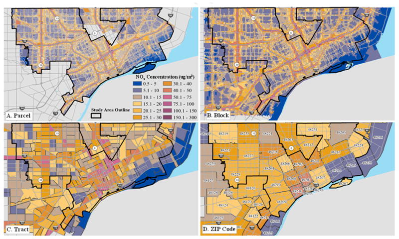
Table 1.
Summary statistics for receptors and four geographic zones for maximum 24-hr NOx concentration (μg/m3). R denotes linear correlation with parcel level data; F2 is factor of two agreement; n=sample size.
| Statistic | Concentrations by Receptor or Zone | ||||
|---|---|---|---|---|---|
|
| |||||
| Receptor | Parcel | Block | Tract | ZIP | |
| Mean | 20.2 | 19.0 | 19.1 | 21.8 | 20.2 |
| Std. Dev | 25.6 | 20.1 | 18.8 | 11.7 | 8.3 |
| Min | 0.5 | 1.4 | 1.4 | 2.0 | 7.8 |
| 10th | 5.4 | 6.9 | 7.1 | 9.6 | 13.7 |
| 25th | 7.8 | 8.7 | 9.0 | 12.1 | 16.5 |
| 50th | 12.0 | 12.8 | 13.2 | 18.8 | 21.1 |
| 75th | 22.0 | 21.1 | 21.4 | 28.6 | 29.0 |
| 90th | 40.6 | 35.7 | 37.2 | 39.4 | 30.6 |
| 99th | 140.0 | 107.0 | 100.3 | 54.5 | 42.0 |
| Max | 299.0 | 299.0 | 299.0 | 64.1 | 45.5 |
| R | - | - | 0.814 | 0.402 | 0.285 |
| F2 | 0.063 | - | 0.005 | 0.138 | 0.154 |
| N | 27,622 | 357,962 | 12,238 | 287 | 25 |
Following from the spatial averaging within each zone, the second effect is a compression of the range of concentrations for the larger zones. For example, the concentration range across receptors and parcels in the study area (1 - 299 μg/m3) was maintained for blocks, but significantly reduced for tracts (10 - 64 μg/m3) and ZIP codes (8 - 45 μg/m3) (Table 1). The cumulative distribution of pollutant levels, weighted by population exposed, shows the significance of these changes (Figure 6). While concentration distributions at receptor, parcel, block, tract and ZIP code levels all varied from one another (Kolmogorov-Smirnov tests, p <0.0001), the largest differences occurred between the three smaller zones and the two larger zones: the larger zones significantly underpredicted the highest 10% of concentrations and completely missed the “extreme” values occurring near major roads. Again, these effects arise from sharp concentration gradients near major roads, as well as land use patterns that avoid the placement of residential property on or very near roads.
Figure 6.

Cumulative distribution of population exposed to maximum 24-hour NOx concentrations estimated at parcel, block, census tract and ZIP code levels.
A third and unanticipated effect was a systematic bias that increased concentrations for the larger zones, seen as a rightward shift of the cumulative exposure distributions (Figure 6) and an increase in median concentrations (e.g., from 13 μg/m3 for parcels to 21 μg/m3 for ZIP codes; Table 1). Parcel-level data largely excluded the on-road microenvironment with the highest concentrations since parcels rarely include roads, especially high traffic roads. In contrast, because the larger zones (e.g., tracts and ZIP codes) comprise the entire zone, areal averages included these high concentrations, and thus residential exposure is overestimated. (Additional descriptions of errors, including an analysis of concentration deviations, are shown in Supplemental Table 1 and Supplemental Figures 4 and 5). As noted, on-road exposure is important for commuters and others who work and travel on high traffic roads, and thus its inclusion may have merit in certain studies. However, because on-road exposure may be shorter in duration, affect a different (e.g., commuting) population, and involve other differences (e.g., pollutant compositional differences, lower breathing rates), including the on-road component in population studies using residence location as an exposure determinant can misclassify exposure, as discussed next.
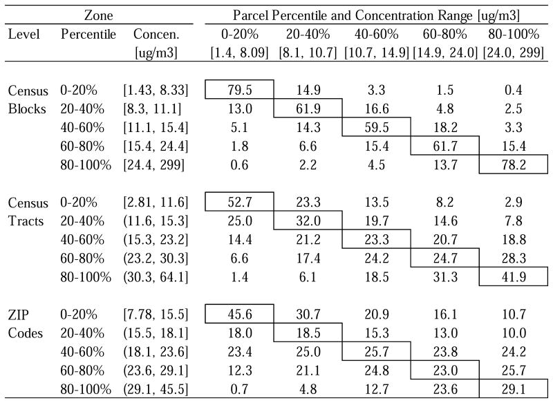
Exposure misclassification rates associated with the use of census blocks, tracts and ZIP codes are shown as off-diagonal values in contingency tables that compare quintiles of population exposure for the highest 24-hr NOx concentration for each zonal system (Table 2). With perfect agreement (i.e., no misclassification), diagonal values (displayed in boxes) would be 100% and off-diagonal values would be 0%. As suggested earlier, census blocks attained the best performance. For example, the top left entry indicates that of the population in the first (lowest) NOx quintile (∼133,000 people exposed to 1.4 to 8.1 μg/m3), blocks correctly classified 79.5% (assuming that the parcel level classification is true). At the block-level, most of the incorrectly classified people were grouped into the second and third quantiles, but 2.4% were classified into the top two exposure quintiles. The overall performance for a zonal system can be taken as the population (or fraction thereof) correctly classified (the average across the diagonal), which is 68, 35, and 28% for blocks, tracts, and ZIP codes, respectively. This analysis shows that performance at tract and ZIP code levels is dismal, e.g., individuals classified into the middle exposure quintile for these zones are nearly equally likely to have low, medium or high exposure; individuals classified into the most-exposed quintile are more likely to have medium and occasionally low exposures. It also shows limits to the simple correlation metrics used earlier, e.g., while correlations appeared high (R = 0.81) between parcel- and block level data, only 68% of the population was correctly classified into quintiles, i.e., nearly one-third of individuals were misclassified.
Table 2.
Contingency table showing agreement and misclassification between population estimates for exposure quintile, showing percentage of population in each quintile. Concentration range shown in parentheses. Boxed percentages would be 100% (and other values 0%) with no exposure misclassification.
|
Exposure misclassification using contingency analyses are more revealing than, or at least complementary to, the correlation and distribution analyses shown earlier (as Table 1, Figure 6) since both the number of persons and the degree of misclassification are displayed. While results depend somewhat on the pollutant metric and classification approach, e.g., number of bins and cut-offs, this analysis strongly reinforces the need for highly spatially resolved exposure data and small geographic units.
4 Recommendations and applications
Analyses in this paper lead to several recommendations regarding traffic-related air pollutant exposure estimates. First, dispersion modeling analyses, which integrate effects of emission, meteorological and locational factors, portray the dramatic temporal and spatial variation – on hourly, daily and seasonal levels – observed for traffic-related air pollutants. This information can be complemented and, to an extent, confirmed by air quality monitoring data if near-road sites are available, although the few monitoring sites typically available cannot show spatial patterns. The choice of averaging time and concentration metric depends on the application. Both short- and long-term metrics might be used to identify “hotspots” and evaluate “critical” locations, e.g., schools, hospitals, parks, and athletic fields where children and other susceptible individuals may be exposed. The present analysis in large part was motivated by the desire for spatially- and temporally-resolved exposure measures in cohort study of children with asthma.
Second, the emission inventory and dispersion modeling indicate that NOx concentrations are dominated by emissions from the larger roads, despite the presence of numerous smaller roads. Results are likely to be similar for other pollutants with several caveats, e.g., significant emissions of volatile organic compounds (VOCs) occur during vehicle start-up and refueling, which is not captured by focusing on major roads. This suggests that focusing on the largest roads may be sufficient to represent many impacts. This would be advantageous as it reduces the data needs and the computational burden, which can be considerable for high-resolution urban scale modeling. However, road alignment must be accurately represented, e.g., short links may be needed to accurately represent curvilinear alignments. Effective means to speed-up computations were presented in the Supplemental Materials.
Third, high spatial resolution is needed to portray the steep concentration gradients found near roads. In modeling applications, receptor grid spacing should be less than 160 m and joining methods using IDW or other averaging techniques are needed to estimate concentrations within 25% of true values at sites as close as 60 to 100 m of major roads; closer spacing is recommended at sites very close to roads. Estimation approaches without averaging, e.g., NN methods, may not perform well, particularly for distances within 40 to 80 m of major roads. The various joining techniques providing comparable area averages for the larger zones, e.g., census tracts and ZIP codes, however, these zones have very limited ability to represent traffic-related air pollutants (discussed further below). These results, obtained for Detroit, emphasize the spatial resolution needed to accurately estimate exposures of traffic-related air pollutants. In other cities and other applications, it may be very difficult to achieve or defend such high resolution. We also show that performance metrics using absolute or relative concentration differences yielded similar trends, although the latter has the advantage of being scale invariant, and that contingency table approach was particularly good at revealing and quantifying exposure misclassification.
Fourth, the zonal systems available and often used in exposure, epidemiology and environmental justice analyses, e.g., data at county, ZIP code, census tract and even census block levels, are poorly suited for investigating traffic-related air pollutants due to the spatial mismatch of concentration gradients and zone sizes. Higher resolution is needed to capture spatial variation. Census block and particularly property parcel-level data are preferred, although long or narrow zones near major roads can produce anomalies, and block-level data produced considerable misclassification, e.g., 32% were misclassified based on the quintile contingency analysis. Unfortunately, high resolution neighborhood-level health indicators are rarely available. The use of larger zones involves several issues: increased rates of misclassification; significantly diminished spatial agreement; compression of the range of concentrations due to area averaging; and systematic overestimation of residential exposure since on- and near-road microenvironments are included. While effects of such errors are context-specific, our results emphasize the need for spatially resolved and preferably geocoded health surveillance and demographic data for evaluating impacts of traffic-related air pollutants.
5 Limitations
The present work has several limitations. First, emission and dispersion modeling involves many parameters, assumptions and input data, and uncertainties can be considerable, particularly for very highly resolved spatial and temporal scales where emissions inventory, meteorological and other model parameters are especially uncertain. While we used the best available information, actual concentrations – and population exposures – will differ from predictions. While absolute levels of predictions involve uncertainties, i.e., factor of roughly two errors are not uncommon due to especially uncertainties in emissions inventories, estimated spatial patterns are likely to be accurate. Thus, dispersion modeling results are sufficient for demonstrating the spatial resolution needed for exposure estimation purposes. Given the extensive input data and computational requirements, examples using such detailed modeling may remain uncommon, unfortunately. Second, concentrations resulting from only primary traffic emissions were considered; secondary pollutants and contributions from other local sources (e.g., power plants, boilers) and from distant sources were omitted. Generally, these other sources are not as important as traffic emissions for NOx, although they may dominate other pollutants, e.g., PM2.5. Third, while the available monitoring data suggests that dispersion modeling results are reasonable, no attempt was made to validate or calibrate models. Fourth, we evaluated a single year. Due to changes in emissions, traffic and meteorology, results may be less relevant for other periods. Fifth, our results are based on a single metropolitan area. While Detroit may be representative of large and predominantly suburban cities, results may differ for areas that are much more or much less densely populated, or those with very different meteorology, terrain and building effects, e.g., street canyons. Sixth, exposure to traffic-related air pollutants most commonly occurs in buildings or in vehicle cabins, and no attempt was made to account for factors influencing indoor-outdoor relationships. Finally, we assumed that parcel-level estimates best reflected exposure, but sub-parcel level variation in activity patterns and other factors may be significant, and it is possible that aggregations at higher spatial scale might provide more accurate exposure estimates.
6 Conclusions
This study has used dispersion modeling to estimate concentrations of traffic-related air pollutants with the aim of improving estimates of population exposure. The modeling portrayed intraurban concentration gradients at a high level of temporal and spatial resolution for a major urban area, and appears to represent the largest and most comprehensive assessment of population exposure in the literature. It shows the need to estimate pollutant levels using essentially the finest-grained zones available for population studies, e.g., property parcel and census block, and the misclassification, biases and reduced variability resulting from larger geographic zones, e.g., tracts, ZIP codes, and counties. A number of recommendations addressing spatial and temporal resolution, as well as computational considerations, are made to help develop accurate exposure estimates. This information is needed for a broad range of studies, e.g., project-level studies designed to characterize hotspots and environmental justice impacts associated with expansion of a freeway, urban- and regional-scale epidemiology studies, and policy-oriented studies, e.g., quantification of energy and pollution trade-offs involved in transit-oriented development. In addition, this information can be used to help evaluate pollution mitigation strategies, e.g., traffic control measures or buffers around highways.
Supplementary Material
Acknowledgments
This research was conducted with input from several partners, including the Community Action Against Asthma (CAAA) Steering Committee, our EPA partners, and the Graham Environmental Sustainability Institute. We thank Veronica Berrocal at the University of Michigan and Kate Blumberg at the International Council for Clean Transportation for their suggestions, and Rich Cook of U.S. EPA's Office of Transportation and Air Quality and Michelle Snyder of UNC Chapel Hill for help in developing locally-resolved traffic emissions. The NEXUS study involves a community-based participatory research partnership, and we thank CAAA and its member organizations.
Funding sources that supported this research included the Graham Environmental Sustainability Institute, the Office of Research and Development at the US Environmental Protection Agency under cooperative agreement R834117 (University of Michigan), and the National Institute of Environmental Health Sciences (NIEHS) through grants 5R01 ESO14677-02 and R01 ES016769-01 for NEXUS. NIEHS provided additional support in grant P30ES017885 “Lifestage exposures and adult disease” as did the Health Effects Institute. Mention of trade names or commercial products does not constitute endorsement or recommendation for use. This article has been reviewed in accordance with U.S. Environmental Protection Agency policy and approved for publication.
Footnotes
Publisher's Disclaimer: This is a PDF file of an unedited manuscript that has been accepted for publication. As a service to our customers we are providing this early version of the manuscript. The manuscript will undergo copyediting, typesetting, and review of the resulting proof before it is published in its final citable form. Please note that during the production process errors may be discovered which could affect the content, and all legal disclaimers that apply to the journal pertain.
Contributor Information
Stuart Batterman, Email: stuartb@umich.edu.
Sarah Chambliss, Email: 2sarah@theicct.org.
Vlad Isakov, Email: Isakov.Vlad@epa.gov.
References
- Apte JS, Bombrun E, Marshall JD, Nazaroff WW. Global intraurban intake fractions for primary air pollutants from vehicles and other distributed sources. Environmental science & technology. 2012;46(6):3415. doi: 10.1021/es204021h. [DOI] [PMC free article] [PubMed] [Google Scholar]
- Barzyk TM, George BJ, Vette AF, Williams RW, Croghan CW, Stevens CD. Development of a distance-to-roadway proximity metric to compare near-road pollutant levels to a central site monitor. Atmospheric Environment. 2009;43(4):787–797. [Google Scholar]
- Batterman S. The near-road ambient monitoring network and exposure estimates for health studies. EM Journal. 2013 Jul;:24–30. [PMC free article] [PubMed] [Google Scholar]
- Bell ML, Morgenstern RD, Harrington W. Quantifying the human health benefits of air pollution policies: Review of recent studies and new directions in accountability research. Environmental Science & Policy. 2011;14(4):357–368. [Google Scholar]
- Brauer M. How Much, How Long, What, and Where. Proceedings of the American Thoracic Society. 2010;7(2):111–115. doi: 10.1513/pats.200908-093RM. [DOI] [PubMed] [Google Scholar]
- Brindley P, Wise SM, Maheswaran R, Haining RP. The effect of alternative representations of population location on the areal interpolation of air pollution exposure. Computers, Environment and Urban Systems. 2005;29(4):455. [Google Scholar]
- Chart-asa C, Sexton KG, Gibson JM. Traffic Impacts on Fine Particulate Matter Air Pollution at the Urban Project Scale: A Quantitative Assessment. Journal of Environmental Protection. 2013;4(12):49. [Google Scholar]
- English P, Neutra R, Scalf R, Sullivan M, Waller L, Zhu L. Examining Associations between Childhood Asthma and Traffic Flow Using a Geographic Information System. Environmental Health Perspectives. 1999;107(9):761. doi: 10.1289/ehp.99107761. [DOI] [PMC free article] [PubMed] [Google Scholar]
- European Environment Agency. The contribution of the transport sector to total emissions of the main air pollutants in 2009 (EEA-32) 2013 Retrieved March 16, 2013, from http://www.eea.europa.eu/data-and-maps/figures/the-contribution-of-the-transport-1.
- Hagler GSW, Baldauf RW, Thoma ED, Long TR, Snow RF, Kinsey JS, Oudejans L, Gullett BK. Ultrafine particles near a major roadway in Raleigh, North Carolina: Downwind attenuation and correlation with traffic-related pollutants. Atmospheric Environment. 2009;43(6):1229–1234. [Google Scholar]
- Health Effects Institute. Traffic-related air pollution: A Critical review of the literature on emissions, exposure, and health effect. Boston, MA: HEI; 2010. [Google Scholar]
- Hoek G, Beelen R, de Hoogh K, Vienneau D, Gulliver J, Fischer P, Briggs D. A review of land-use regression models to assess spatial variation of outdoor air pollution. Atmospheric Environment. 2008;42(33):7561. [Google Scholar]
- Hu SS, Fruin S, Kozawa K, Mara S, Paulson SE, Winer AM. A wide area of air pollutant impact downwind of a freeway during pre-sunrise hours. Atmospheric Environment. 2009;43(16):2541–2549. doi: 10.1016/j.atmosenv.2009.02.033. [DOI] [PMC free article] [PubMed] [Google Scholar]
- Huang YL, Batterman S. Residence location as a measure of environmental exposure: a review of air pollution epidemiology studies. Journal of Exposure Analysis and Environmental Epidemiology. 2000;10(1):66. doi: 10.1038/sj.jea.7500074. [DOI] [PubMed] [Google Scholar]
- Hystad P, Setton E, Cervantes A, Poplawski K, Deschenes S, Brauer M, van Donkelaar A, Lamsal L, Martin R, Jerrett M, Demers P. Creating National Air Pollution Models for Population Exposure Assessment in Canada. Environmental Health Perspectives. 2011;119(8):1123. doi: 10.1289/ehp.1002976. [DOI] [PMC free article] [PubMed] [Google Scholar]
- Isakov V, Touma JS, Burke J, Lobdell DT, Palma T, Rosenbaum A, Ozkaynak H. Combining regional- and local-scale air quality models with exposure models for use in environmental health studies. J Air Waste Manag Assoc. 2009;59(4):461–472. doi: 10.3155/1047-3289.59.4.461. [DOI] [PubMed] [Google Scholar]
- Jerrett M, Arain A, Kanaroglou P, Beckerman B, Potoglou D, Sahsuvaroglu T, Morrison J, Giovis C. A review and evaluation of intraurban air pollution exposure models. Journal of exposure analysis and environmental epidemiology. 2005;15(2):185. doi: 10.1038/sj.jea.7500388. [DOI] [PubMed] [Google Scholar]
- Jin T, Fu L. Application of GIS to modified models of vehicle emission dispersion. Atmospheric Environment. 2005;39(34):6326. [Google Scholar]
- Karner AA, Eisinger DS, Niemeier DA. Near-roadway air quality: synthesizing the findings from real-world data. Environ Sci Technol. 2010;44(14):5334–5344. doi: 10.1021/es100008x. [DOI] [PubMed] [Google Scholar]
- Laumbach RJ, Kipen HM. Respiratory health effects of air pollution: update on biomass smoke and traffic pollution. Journal of Allergy & Clinical Immunology. 2012;129(1):3–11. doi: 10.1016/j.jaci.2011.11.021. quiz 12-13. [DOI] [PMC free article] [PubMed] [Google Scholar]
- Lin MD, Lin YC. The application of GIS to air quality analysis in Taichung City, Taiwan, ROC. Environmental Modelling and Software. 2002;17(1):11. [Google Scholar]
- Lipfert FW, Wyzga RE. On exposure and response relationships for health effects associated with exposure to vehicular traffic. Journal of Exposure Science and Environmental Epidemiology. 2008;18(6):588. doi: 10.1038/jes.2008.4. [DOI] [PubMed] [Google Scholar]
- Lobdell DT, Isakov V, Baxter L, Touma JS, Smuts MB, Ozkaynak H. Feasibility of assessing public health impacts of air pollution reduction programs on a local scale: New Haven case study. Environmental Health Perspectives. 2011;119(4):487–493. doi: 10.1289/ehp.1002636. [DOI] [PMC free article] [PubMed] [Google Scholar]
- McKenzie B, Melanie R. American Community Survey Reports, ACS-15. Washington, DC: U.S. Census Bureau; 2011. Commuting in the United States: 2009. [Google Scholar]
- Molitor J, Jerrett M, Chang CC, Molitor NT, Gauderman J, Berhane K, McConnell R, Lurmann F, Wu J, Winer A, Thomas D. Assessing uncertainty in spatial exposure models for air pollution health effects assessment. Environmental Health Perspectives. 2007;115(8):1147–1153. doi: 10.1289/ehp.9849. [DOI] [PMC free article] [PubMed] [Google Scholar]
- Okabe A, Sadahiro Y. Variation in count data transferred from a set of irregular zones to a set of regular zones through the point-in-polygon method. International Journal of Geographical Information Science. 1997;11(1):93. [Google Scholar]
- Sharma P, Khare M. Modelling of vehicular exhausts – a review. Transportation Research Part D. 2001;6(3):179. [Google Scholar]
- Sheppard LR, Burnett T, Szpiro AA, Kim SY, Jerrett M, Pope CA, Iii, Brunekreef B. Confounding and exposure measurement error in air pollution epidemiology. Air Quality, Atmosphere & Health. 2012;5(2):203. doi: 10.1007/s11869-011-0140-9. [DOI] [PMC free article] [PubMed] [Google Scholar]
- Snyder MG, Venkatram A, Heist DK, Perry SG, Petersen WB, Isakov V. RLINE: A line source dispersion model for near-surface releases. Atmospheric Environment. 2013;77(0):748–756. [Google Scholar]
- Tian N, Xue J, Barzyk TM. Evaluating socioeconomic and racial differences in traffic-related metrics in the United States using a GIS approach. Journal of exposure science & environmental epidemiology. 2013;23(2):215. doi: 10.1038/jes.2012.83. [DOI] [PubMed] [Google Scholar]
- U.S. Department of Housing and Urban Development and U.S. Department of Commerce. American Housing Survey for the United States: 2009 2011 [Google Scholar]
- U.S. Environmental Protection Agency. Integrated Science Assessment for Oxides of Nitrogen – Health Criteria. Research Triangle Park, NC: National Center for Environmental Assessment, Office of Research and Development; 2008. [Google Scholar]
- U.S. Environmental Protection Agency. National Summary of Nitrogen Oxides Emissions, NEI 2008. 2013 Retrieved April 16, 2013, from http://www.epa.gov/cgi-bin/broker?polchoice=NOX&_debug=0&_service=data&_program=dataprog.national_1.sas.
- Venkatram A, Snyder MG, Heist DK, Perry SG, Petersen WB, Isakov V. Reformulation of plume spread for near-surface dispersion. Atmospheric Environment. 2013;77(0):846–855. [Google Scholar]
- Vette A, Burke J, Norris G, Landis M, Batterman S, Breen M, Isakov V, Lewis T, Gilmour MI, Kamal A, Hammond D, Vedantham R, Bereznicki S, Tian N, Croghan C. The Near-Road Exposures and Effects of Urban Air Pollutants Study (NEXUS): study design and methods. The Science of the total environment. 2013;448:38. doi: 10.1016/j.scitotenv.2012.10.072. [DOI] [PMC free article] [PubMed] [Google Scholar]
- Wilson JG, Kingham S, Pearce J, Sturman AP. A review of intraurban variations in particulate air pollution: Implications for epidemiological research. Atmospheric Environment. 2005;39(34):6444. [Google Scholar]
- Wu YC, Batterman SA. Proximity of schools in Detroit, Michigan to automobile and truck traffic. Journal of Exposure Science and Environmental Epidemiology. 2006;16(5):457–470. doi: 10.1038/sj.jes.7500484. [DOI] [PubMed] [Google Scholar]
Associated Data
This section collects any data citations, data availability statements, or supplementary materials included in this article.