A Deterministic Model Predicts the Properties of Stochastic Calcium Oscillations in Airway Smooth Muscle Cells

Abstract

The inositol trisphosphate receptor () is one of the most important cellular components responsible for oscillations in the cytoplasmic calcium concentration. Over the past decade, two major questions about the have arisen. Firstly, how best should the be modeled? In other words, what fundamental properties of the allow it to perform its function, and what are their quantitative properties? Secondly, although calcium oscillations are caused by the stochastic opening and closing of small numbers of , is it possible for a deterministic model to be a reliable predictor of calcium behavior? Here, we answer these two questions, using airway smooth muscle cells (ASMC) as a specific example. Firstly, we show that periodic calcium waves in ASMC, as well as the statistics of calcium puffs in other cell types, can be quantitatively reproduced by a two-state model of the , and thus the behavior of the is essentially determined by its modal structure. The structure within each mode is irrelevant for function. Secondly, we show that, although calcium waves in ASMC are generated by a stochastic mechanism, stochasticity is not essential for a qualitative prediction of how oscillation frequency depends on model parameters, and thus deterministic models demonstrate the same level of predictive capability as do stochastic models. We conclude that, firstly, calcium dynamics can be accurately modeled using simplified models, and, secondly, to obtain qualitative predictions of how oscillation frequency depends on parameters it is sufficient to use a deterministic model.

Author Summary

The inositol trisphosphate receptor () is one of the most important cellular components responsible for calcium oscillations. Over the past decade, two major questions about the have arisen. Firstly, what fundamental properties of the allow it to perform its function? Secondly, although calcium oscillations are caused by the stochastic properties of small numbers of is it possible for a deterministic model to be a reliable predictor of calcium dynamics? Using airway smooth muscle cells as an example, we show that calcium dynamics can be accurately modeled using simplified models, and, secondly, that deterministic models are qualitatively accurate predictors of calcium dynamics. These results are important for the study of calcium dynamics in many cell types.

Introduction

Oscillations in cytoplasmic calcium concentration (), mediated by inositol trisphosphate receptors (; a calcium channel that releases calcium ions () from the endoplasmic or sarcoplasmic reticulum (ER or SR) in the presence of inositol trisphosphate ()) play an important role in cellular function in many cell types. Hence, a thorough knowledge of the behavior of the is a necessary prerequisite for an understanding of intracellular oscillations and waves. Mathematical and computational models of the play a vital role in studies of dynamics. However, over the past decade, two major questions about models have arisen.

Firstly, how best should the be modeled? Models of the have a long history, beginning with the heuristic models of [1]–[3]. With the recent appearance of single-channel data from in vivo [4], [5], a new generation of Markov models has recently appeared [6], [7]. These models show that exist in different modes with different open probabilities. Within each mode there are multiple states, some open, some closed. Importantly, it was found [8] that time-dependent transitions between different modes are crucial for reproducing puff data from [9]. However, it is not yet clear whether transitions between states within each mode are important, or whether all the important behaviors are captured simply by inter-mode transitions.

Secondly, why do deterministic models of the perform so well as predictive models? Deterministic models of the have proven to be useful predictive models in a range of cell types. For example, -based models have been developed to study oscillations in airway smooth muscle cells (ASMC) [10]–[13], and these models have made predictions which have been confirmed experimentally. This shows the usefulness of such models in advancing our understanding of how intracellular oscillations and waves are initiated and controlled in ASMC. However, these models are deterministic models which assume infinitely many per unit cell volume, an assumption that contradicts experimental findings in many cell types showing that puffs and spikes occur stochastically, and that intracellular waves and oscillations arise as an emergent property of fundamental stochastic events [9], [14], [15].

Here, we answer these two fundamental modeling questions using data and models from ASMC. Firstly, we show that a simple model of the , involving only two states with time-dependent transitions, suffices to generate correct dynamics of puffs and oscillations. Secondly, we show that, although oscillations in ASMC are generated by a stochastic mechanism, a deterministic model can make the same qualitative predictions as the analogous stochastic model, indicating that deterministic models, that require much less computational time and complexity, can be used to make reliable predictions. Although we work in the specific context of ASMC, our results are applicable to other cell types that exhibit similar oscillations and waves.

Results

A two-state model of the is sufficient to reproduce function

We have previously shown [8] that the statistics of puffs in SH-SY5Y cells can be reproduced by a Markov model of the based on the steady-state data of [5] and the time-dependent data of [4]. In this model the can exist in 6 different states, grouped into two modes, which we call Drive and Park (see Fig. 1). The Drive mode (which contains 4 states; 1 open and 3 closed) has an average open probability of around 0.7, while the Park mode (which contains the remaining two states; 1 open and 1 closed) has an open probability close to zero. Transitions between states within each mode are independent of and ; only the transitions between modes are ligand-dependent.

Figure 1. The structure of the Siekmann model.

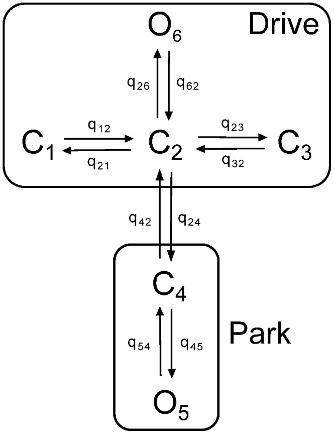
The model is comprised of two modes. One is the drive mode containing three closed states , , and one open state . The other is the park mode which includes one closed state and one open state . are rates of state-transitions between two adjacent states and and are transitions between the two modes [7].

In our previous study on calcium puffs [8], we showed that, to reproduce the experimentally observed non-exponential interspike interval (ISI) distribution and coefficient of variation (CV) of ISI smaller than 1, the time-dependent intermodal transitions are crucial. Lack of time dependencies in the Siekmann model leads to exponential ISI distributions and CV = 1, which is not the case for calcium spikes in ASMC. Fig. 2A shows an example of oscillations generated by 50 nM methacholine (MCh, an agonist that can induce the production of by binding to a G protein-coupled receptor in the cell membrane) in ASMC. By gathering data from 14 cells in 5 mouse lung slices, we found that the standard deviation of the interspike interval (ISI) is approximately a linear function of the ISI mean, with a slope clearly between 0 and 1 (i.e. ), indicating that the spikes are generated by an inhomogeneous Poisson process (a slope of 1 would denote a pure Poisson process) (see Fig. 2B). This shows the necessity of inclusion of time-dependent transitions for mode-switching.

Figure 2. oscillations in ASMC in lung slices are generated by a stochastic mechanism.

A: experimental spiking in ASMC in lung slices, stimulated with 50 nM MCh. In the upper panel we filter out baseline noise by using a low threshold of 1.42 (relative fluorescence intensity) and then choose samples with amplitude larger than 1.75. The ISI calculated from the upper panel is shown in the lower panel. B: relationship between the standard deviation and the mean of experimental ISIs. Data obtained from 14 ASMC in 5 mouse lung slices. The relationship is approximately linear with a slope of 0.66, which implies that an inhomogeneous Poisson process governs the generation of oscillations. The dashed line indicates where the coefficient of variation (CV) is 1 (as it is for a pure Poisson process). Variation in ISI is mainly caused by both use of different doses of MCh and different sensitivities of different cells to MCh. Error bars indicate the standard errors of the means (SEM).

Using a quasi-steady-state approximation, and ignoring states with very low dwell times, it is possible to construct a simplified two-state version of the full six-state model (see Materials and Methods ). In the simplified model the intramodal structure is ignored, and only the intermodal transitions have an effect on behavior. In Fig. 3 we compared the simplified model to the full six-state model. Both models have the same distribution of interspike interval, spike amplitude and spike duration. Moreover, by looking at a more detailed comparison between the two model results (Figs. 4A, C and E) and experimental data (Figs. 4B, D and F), we found the 2-state model not only can reproduce the behaviour of the 6-state model, but can also qualitatively reproduce experimental data. The average experimental ISI shows a clear decreasing trend as MCh concentration increases (although a saturation occurs in the data for high MCh), a trend that is mirrored by the model results as the concentration increases. Unfortunately, since the exact relationship between MCh concentration and concentration is uncertain, a quantitative comparison is not possible. In both model and experimental results, the average peak and duration of the oscillations are nearly independent of agonist concentration. The quantitative difference in spike duration between the model results and the data in Figs. 4E and F are most likely due to choice of calcium buffering parameters. For example, adding fast buffer (see Materials and Methods ) increases the average spike duration to 0.54 s or 0.7 s respectively, which are close to the levels shown in the data.

Figure 3. A 2-state open/closed model quantitatively reproduces the 6-state model.

A: histograms of interspike interval (ISI) distribution for both the 6-state and the simplified models. The ISI is defined to be the waiting time between successive spikes. Each histogram contain an equal number of samples (180). B: comparison of average ISI, average peak value of ( in the model) and average spike duration. All distributions were computed at a constant .

Figure 4. More detailed comparisons between the 2-state and the 6-state models, and a comparison to experimental data.

As a function of concentration (), the two models give the same ISI (A), peak (C) and spike duration (E). These results agree qualitatively with experimental data, as shown in panels B, D and F respectively. Quantitative comparisons are generally not possible as the relationship between concentration and agonist concentration is not known. Error bars represent . Data for each MCh concentration are obtained from at least three different cells from at least two different lung slices.

Thus, the intramodal structure of the six-state model is essentially unimportant, as the model behavior (in terms of the statistics of puffs and oscillations) is governed almost entirely by the time dependence of the intermode transitions, particularly the time dependence of the rapid inhibition of the by high , and the slow recovery from inhibition by . The multiple states within each mode are necessary to obtain an acceptable quantitative fit to single-channel data, but are nevertheless of limited importance for function. Hence, even when simulating microscopic events such as puffs it is sufficient to use a simpler, faster, two-state model, rather than a more complex six-state model. In the following, we will use the 2-state model to generate all the simulation results.

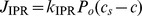
Prediction of stochastic behavior by a deterministic model

Although the data (Fig. 2) show that oscillations in ASMC are generated by a stochastic process, not a deterministic one, we wish to know to what extent a deterministic model can be used to make qualitative (and experimentally testable) predictions. Our simplified 2-state Markov model of the can be converted to a deterministic model (see Materials and Methods ). The result is a system of ordinary differential equations (ODEs) with four variables, which takes into account the increased at an open pore, as well as the increased within a cluster of ; the four variables are the outside the cluster (), the within the cluster (), the total intracellular concentration () and an gating variable (). We refer to the reduced 4D model as the deterministic model for all the results and analyses.

Note that there is no physical or geometric constraint enforcing a high local ; in this case the spatial heterogeneity arises solely from the low diffusion coefficient of . Our use of is merely a highly simplified way of introducing spatial heterogeneity of the concentration. Since the can only “see” (as well as the concentration right at the mouth of an open channel, which we denote by ), but cannot be influenced directly by (the experimentally observed signal), our approach allows for the functional differentiation of the rapid local oscillatory in the cluster, from the slower signal in the cytoplasm, without the need for computationally intensive simulations of a partial differential equation model. Quantitative accuracy is thus sacrificed for computational convenience.

Calcium oscillations in the stochastic and deterministic models are shown in Fig. 5A. According to our previous results [8], the average value of over the cluster of primarily regulates the termination and regeneration of individual spikes. This can be seen in the stochastic model by projecting the solution on the phase plane (Fig. 5B). Upon an initial release from one or more , a large spike is generated by Ca²⁺-induced release (via the ) during which time a decreasing gradually decreases the average open probability of the clustered . The spike is terminated when is too small to allow further release. This phenomenon is qualitatively reproduced by the deterministic model (Fig. 5D). In both the stochastic and deterministic models the decrease in average open probability of a cluster of caused by inhibition is the main reason for the termination of each spike.

Figure 5. Stochastic and deterministic simulations exhibit similar dynamic properties.

A: simulated stochastic (upper panel) or deterministic (lower panel) oscillations at . B: a typical stochastic solution projected on the plane. The average represents the average value of over the 20 . Statistics () of the initiation point (blue square), the peak (red square) and termination point (green square) are shown in the inset. 116 samples are obtained by applying a low threshold of and a high threshold of to . C: a typical periodic solution of the deterministic model (black curve), plotted in the phase space. The arrow indicates the direction of movement. is the slowest variable so that its variation during an oscillation is very small. This allows to treat as a constant ( in this case) and study the dynamics of the model in the phase space. The color surface is the surface where (called the critical manifold). The white N-shaped curve is the intersection of the critical manifold and the surface . D: projection of the periodic solution to the plane. The red N-shaped curve is the projection to the plane of the white curve shown in C. The evolution of the deterministic solution exhibits three different time scales separated by green circles (labelled by a, b and c) and indicated by arrows (triple arrow: fastest; double arrow: intermediate; single arrow: slowest).

According to Figs. 5B and D, regeneration of each spike requires a return of back to a relatively high value (i.e., recovery of the from inhibition by ). The deterministic model sets a clear threshold for the regeneration, as can be seen in Fig. 5C, where an upstroke in occurs when the trajectory creeps beyond the sharp “knee” of the white curve. When the trajectory reaches the knees of the white curve it is forced to jump across to the other stable branch of the critical manifold, resulting in a fast increase in followed by a relatively fast increase in (seen by combining Figs. 5C and D).

In contrast, the stochastic model enlarges the contributions of individual so that the generation of each spike is also effectively driven by random release through the , which can be seen in the inset of Fig. 5B where the site of spike initiation (blue bar) exhibits significantly greater variation than that of spike termination (green bar). In spite of this, the essential similarities in phase plane behavior result in both deterministic and stochastic models making the same qualitative predictions in response to perturbations, such as changes in concentration (), influx or efflux. In the following, we illustrate this by investigating a number of experimentally testable predictions. Due to the extensive importance of frequency encoding in many -dependent processes, we focus particularly on the change of oscillation frequency in response to parameter perturbations. As a side issue we also investigate how the oscillation baseline depends on physiologically important parameters.

Dependence of oscillation frequency on concentration

In many cell types a moderate increase in increases the oscillation frequency (see Fig. 2A in [11], Fig. 4E in [16] and Fig. 6B in [17]), a result that is reproduced by both model types (Fig. 6A). As increases, the stochastic model increases the probability of the initial release through the first open and of the following release, thus shortening the average ISI. Although the oscillatory region of the deterministic model is strictly confined by bifurcations which do not apply to the stochastic model, the deterministic model can successfully replicate an increasing frequency by lowering the “knee” of the red curve in Fig. 5D and shortening the time spent from the termination point c to the initiation point a (thus shortening the ISI). Hence, although the deterministic model cannot be used to predict the exact values of at which the oscillations begin and end, as stochastic effects predominate in these regions, it can be used to predict the correct qualitative trend in oscillation frequency.

Figure 6. Comparison of parameter-dependent frequency changes in the stochastic and deterministic models.

All curves are computed at except in panel A, which uses a variety of . Other parameters are set at their default values given in Table 1. A: as increases, oscillations in both models increase in frequency. B: as influx increases (modeled by an increase in receptor-operated calcium channel flux coefficient ), so does the oscillation frequency in both models. C: as efflux increases (modeled by an increase in plasma pump expression ), oscillation frequency decreases. D: as SERCA pump expression, , increases, so does oscillation frequency. E: as total buffer concentration, , increases, oscillation frequency decreases.

Dependence of oscillation frequency on influx and efflux

In many cell types, including ASMC, transmembrane fluxes modulate the total intracellular load () on a slow time scale [16], [18], and thereby modulate the oscillation frequency [19]. Experimental data can be seen in Fig. 8 in [16] and Fig. 2 in [18]. Figs. 6B and C show that both stochastic and deterministic models predict the same qualitative changes in oscillation frequency in response to changes in membrane fluxes (through membrane ATPase pumps and/or influx channels such as receptor-operated channels or store-operated channels).

Figure 8. Schematic diagram of the model.

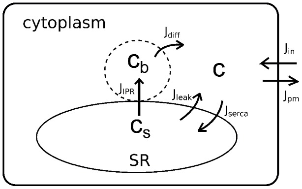
represents cytoplasmic concentration, excluding a small local (whose concentration is denoted by ) close to the release site (i.e., an cluster). Upon coordinated openings of the , SR () is first released into the local domain () to cause a rapid increase in . High local then diffuses to the rest of the cytoplasm (), and is eventually pumped back to the SR ().

Dependence of oscillation frequency on SERCA expression

The level of sarco/endoplasmic reticulum calcium ATPase (SERCA) expression (or capacity) is important for airway remodeling in asthma [20] and ASMC oscillations [21]. We thus investigated the predictions of the two models in response to changes in SERCA expression (). As decreases, the deterministic model exhibits a decreasing frequency, in agreement with experimental data (see Figs. 3 and 4 in [21]). The same trend is seen in the stochastic model with only 20 (see Fig. 6D).

Dependence of oscillation frequency on buffer concentration

Calcium buffers have been shown to be able to change the ISI and spike duration, which in turn change the oscillation frequency [15], [22]. We compared the effects on the two models of varying total buffer concentration () by adding one buffer with relatively fast kinetics to the models (see Materials and Methods for details). In both models the frequency decreases as increases (see Fig. 6E), which is consistent with experimental data (Fig. 2B in [18]). This is not surprising, because increasing can decrease the effective rates of SR release and reuptake.

Dependence of oscillation baseline on influx and SERCA expression

Sustained elevations of baseline during agonist-induced oscillations or transients have been observed experimentally, and are believed to be a result of an increase in influx caused by opening of membrane channels [13], [16]. Furthermore, there is evidence showing that decreased SERCA expression could also increase the baseline (Fig. 4 in [21]). Those phenomena are successfully reproduced by both models (see Fig. 7).

Figure 7. Dependence of calcium oscillation baseline on calcium influx and SERCA expression.

A: increasing influx (described by ) increases the average trough of oscillations. B: decreasing SERCA expression (described by ) increases the average trough of oscillations. All curves are computed at .

Discussion

In this paper we address two current major questions in the field of modeling. Firstly, we show that puffs and stochastic oscillations can be reproduced quantitatively by an extremely simple model, consisting only of two states (one open, one closed), with time-dependent transitions between them. This model is obtained by removing the intramodal structure of a more complex model that was determined by fitting a Markov model to single-channel data [7]. We thus show that the internal structure of each mode is irrelevant for function and mode switching is the key mechanism for the control of calcium release. The necessity for time-dependent mode switching is shown not only by the dynamic single-channel data of [4]), but also by the puff data of [9] and our ASMC data.

Secondly, we investigate the role of stochasticity of in modeling oscillations in ASMC by comparing a stochastic IP₃R-based model and its associated deterministic version, for parameters such that both of the models exhibit spikes but the stochastic model cannot necessarily be replaced by a mean-field model. We find that a four-variable deterministic model has the same predictive power as the stochastic model, in that it correctly reproduces the process of spike termination and predicts the same qualitative changes in oscillation frequency and baseline in response to a variety of perturbations that are commonly used experimentally. The mechanism for termination of individual spikes is fundamentally a deterministic process controlled by a rapid inhibition induced by the high local in the cluster, whereas spike initiation is significantly affected by stochastic opening of . Hence, repetitive cycling is primarily induced by the time-dependent gating variables governing transitions of the from one mode to another.

Our simplified two-state model of the is identical in structure (although not in parameter values) to the well-known model of [23]. It is somewhat ironic that after 20 years of detailed studies of the and the construction of a plethora of models of varying complexity, the single-channel data have led us around full circle, back to these original formulations. Excitability is arising via a fast activation followed by a slower inactivation, a combination often seen in physiological processes [24]. Encoding of this fundamental combination results directly from the two-mode structure of the . Although similar single-channel data have been used to construct three-mode models [6], [25], neither of these models has yet been used in detailed studies of puffs and waves, and it remains unclear whether or not they have a similar underlying structure.

In contrast to previous deterministic ODE models, our four-variable model includes a more accurate model, as well as local control of clustered by two distinct microdomains; one at the mouth of an open , the other inside a cluster of . Neglect of either of these microdomains leads to models that either exhibit unphysiological cytoplasmic concentrations or fail to reproduce reasonable oscillations. This underlines the importance of taking microdomains into consideration when constructing any model. Our microdomain model is highly simplified, with the microdomain being treated simply as a well-mixed compartment. More detailed modeling of spatially-dependent microdomains is possible, and not difficult in principle, but requires far greater computational resources. It is undeniable that a more detailed model, incorporating the full spatial complexity – and possibly stochastic aspects as well – would make, overall, a better predictive tool. However, our goal is to find the simplest models that can be used as predictive tools.

An important similar study is that of Shuai and Jung [26]. They compared the use of Markov and Langevin approaches to the computation of puff amplitude distributions, compared their results with the deterministic limit, and showed that stochasticity does not qualitatively change the type of puff amplitude distribution except for when there are fewer than 10 . Here, we significantly extend the scope of their study by exploring the effects of stochasticity on the dynamics of spikes, and we do this in the context of an model that has been fitted to single-channel data. Although this is true in a general sense for the Li-Rinzel model, which is based on the DeYoung-Keizer model, which did take into account the opening time distributions of in lipid bilayers, neither model can reproduce the more recent data obtained from on-nuclei patch clamping. When these recent data are taken into account one obtains a model with the same structure, but quite different parameters and behavior.

We find that, in spite of a relatively large variation in spike amplitude which is partially caused by a large variation in ISI (Fig. 5B), the mechanism governing individual spike terminations is the same for both a few or infinitely many , which explains why the one-peak type of amplitude distribution is independent of the choice of number (see Fig. 6A in [26]).

Another important relevant study was done by Dupont et al. [27], who compared the regularity of stochastic oscillations in hepatocytes for different numbers of clusters. They found that the impact of stochasticity on global oscillations (in terms of CV) increases as the total cluster number decreases. Our study here extends these results, and demonstrates how well stochastic oscillations can be qualitatively described by a deterministic system, even when there is only a small number of (which appears to be the case for ASMC, in which the wave initiation site is only in diameter). Indeed, as we have shown, for the purposes of predictive modeling a simple deterministic model does as well as more complex stochastic simulations.

Ryanodine receptors (RyR) are another important component modulating ASMC oscillations [16], [28], [29] but are not included in our model. This is because the role of RyR is not fully understood and may be species-dependent; for example, in mouse or human ASMC, RyR play very little role in -induced continuing oscillations [17], [30], but this appears not to be true for pigs [28]. Our study focuses on the calcium oscillations in mouse and human (as we did in our experiments) where inclusion of a deterministic model of RyR should have little effect. An understanding of the role of RyR stochasticity and how the and the RyR interact needs a reliable RyR Markov model, exclusive to ASMC, which is not currently available. Multiple Markov models of the RyR have been developed for use in cardiac cells [31], but these are based on single-channel data from lipid bilayers, and are adapted for the specific context of cardiac cells. Their applicability to ASMC remains unclear.

Although we have not shown that the deterministic model for ASMC has the same predictive power as the stochastic model in all possible cases (which would hardly be possible in the absence of an analytical proof) the underlying similarity in phase plane structure indicates that such similarity is plausible at least. Certainly, we have not found any counterexample to this claim. However, whether or not this claim is true for all cell types is unclear. Some cell types exhibit both local puffs and global spikes (usually propagating throughout the cells in the form of traveling waves), showing that initiation of such spikes requires a synchronization of release from more than one cluster of [14]. This type of spiking relies on the hierarchical organization of signal pathways, in particular the stochastic recruitment of both individual and puffs at different levels [32], and therefore cannot be simply reproduced by deterministic models containing only a few ODEs. However, oscillations in ASMC, as observed in lung slices, may not be of this type, as IP₃R-dependent puffs have not been seen in these ASMC. It thus appears that, in ASMC in lung slices, every “puff” initiates a wave, resulting in periodic waves with ISI that are governed by the dynamics of individual puffs.

Materials and Methods

Ethics Statement

Animal experimentations carried out were approved by the Animal Care and Use Committee of the University of Massachusetts Medical School under approval number A-836-12.

Lung slice preparation

BALB/c mice (7–10 weeks old, Charles River Breeding Labs, Needham, MA) were euthanized via intraperitoneal injection of 0.3 ml sodium pentabarbitone (Oak Pharmaceuticals, Lake Forest, IL). After removal of the chest wall, lungs were inflated with of 1.8% warm agarose in sHBSS via an intratracheal catheter. Subsequently, air () was injected to push the agarose within the airways into the alveoli. The agarose was polymerized by cooling to . A vibratome (VF-300, Precisionary Instruments, San Jose, CA) was used to make thick slices which were maintained in Dulbecco's Modified Eagle's Media (DMEM, Invitrogen, Carlsbad, CA) at in /air. All experiments were conducted at in a custom-made temperature-controlled Plexiglas chamber as described in [17].

Measurement of oscillations

Lung slices were incubated in sHBSS containing Oregon Green 488 BAPTA-1-AM (Invitrogen), a Ca²⁺-indicator dye, 0.1% Pluronic F-127 (Invitrogen) and sulfobromophthalein (Sigma Aldrich, St Louis, MO) in the dark at for 1 hour. Subsequently, the slices were incubated in sulfobromophthalein for 30 minutes. Slices were mounted on a cover-glass and held down with mesh. A smaller cover-glass was placed on top of the mesh and sealed at the sides with silicone grease to facilitate solution exchange. Slices were examined with a custom-built 2-photon scanning laser microscope with a oil immersion objective lens and images recorded at 30 images per second using Videosavant 4.0 software (IO Industries, Montreal, Canada). Changes in fluorescence intensity (which represent changes in ) were analyzed in an ASMC of interest by averaging the grey value of a pixel region using custom written software. Relative fluorescence intensity () was expressed as a ratio of the fluorescence intensity at a particular time (F) normalized to the initial fluorescence intensity ().

The calcium model

Inhomogeneity of cytoplasmic concentration not only exists around individual channel pores of the , where a nearly instantaneous high concentration at the pore (denoted by ) leads to a very sharp concentration profile, but is also seen inside an cluster where the average cluster concentration () is apparently higher than that of the surrounding cytoplasm () [33]. This indicates that during oscillations each is controlled by either the pore concentration (when it is open) or the cluster concentration (when it is closed). Neither of these local concentrations influence cell membrane fluxes or the majority of SERCAs, which we assume to be distributed outside the cluster.

The scale separation between the pore concentration and the cluster concentration allows to treat as a parameter, providing a simpler way of modeling local events (like puffs) that has been used in several previous studies [8], [34], [35]. However, evolution of the cluster concentration and wide-field cytoplasm concentration are not always separable, so an additional differential equation for the cluster is necessary.

A schematic diagram of the model is shown in Fig. 8. The corresponding ODEs are

(1)

(2)

(3)

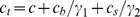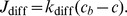
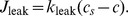
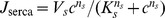
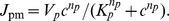
where representing total intracellular concentration, and thus SR concentration, is given by . and are the volume ratios given in Table 1. is the flux through the , is a background leak out of the SR, and is the uptake of into the SR by SERCA pumps. is the flux through plasma pump, and represents a sum of main influxes including (receptor-operated channel), (store-operated channel) and ( leak into the cell). coarsely models the diffusion flux from cluster microdomain to the cytoplasm. Details of the fluxes are

Table 1. Parameter values of the stochastic calcium model.

Parameter	Description	Value/Units
	flux coefficient
	diffusional flux coefficient
	SR leak flux coefficient
	maximum capacity of SERCA
	SERCA half-maximal activating
	Hill coefficient for SERCA	1.75
	plasma membrane leak influx
	ROCC flux coefficient
	maximum capacity of SOCC
	SOCC dissociation constant
	maximum capacity of plasma pump
	half-maximal activating of plasma pump
	Hill coefficient for plasma pump	2
	the cytoplasmic-to-microdomain volume ratio	100
	the cytoplasmic-to-SR volume ratio	10
	an instantaneous high at open channel pore when
	total number of channels	20

• • Different formulations of give different types of models:

  • a) For the stochastic model, where is the maximum conductance of a cluster of (here ). is the number of open determined by the states of .

  • b) For the deterministic model we set where is the open probability, a continuous analogue of .

  To calculate and , we use the model of [7], [8], with minor modifications described later.

• •

• • where and are obtained from [36].

• •

• • includes a basal leak (), receptor-operated calcium channel (ROCC, ), store-operated calcium channel (SOCC, ). By using the concentration () as a surrogate indicator of MCh concentration, we assume that . SOCC is modeled by [13].

• •

Calcium concentration at open channel pore () does not explicitly appear in the equations but is used in the model introduced later. is assumed to be proportional to SR concentration () and is therefore simply modeled by 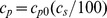where is the value corresponding to . Alternatively, can also be assumed to be a large constant (say greater than ) without fundamentally altering the model dynamics. The choice of is not critical as long as it is sufficiently large to play a role in inactivating the open channels. All the parameter values are given in Table 1.

The data-driven model

The model used in our ASMC calcium model is an improved version of the Siekmann model which is a 6-state Markov model derived by fitting to the stationary single channel data using Markov chain Monte Carlo (MCMC) [5], [7], [8]. Fig. 1 has shown the structure of the model which is comprised of two modes; the drive mode, containing three closed states , , and one open state , and the park mode, containing one closed state and one open state . The transition rates in each mode are constants (shown in Table 2), but and which connect the two modes are -/-dependent and are formulated as

(4)

(5)

where , , and are -/-modulated gating variables. , , and are either functions of or constants and are given later. We assume the gating variables obey the following differential equation,

(6)

where is the equilibrium and is the rate at which the equilibrium is approached. Those equilibria are functions of concentration at the cytoplasmic side of the , denoted by in the equations, equal to either or depending on the state of the channel). They are assumed to be

(7)

(8)

(9)

(10)

Table 2. Parameter values of the model.

Parameter	Value/Units	Parameter	Value/Units

Hence, we have stationary expressions of and ,

(11)

(12)

The expressions of s, s, s and s are chosen as follows so that Eq. 11 and Eq. 12 capture the correct trends of experimental values of and (see Fig. 9) and generate relatively smooth open probability curves (see Fig. 10),

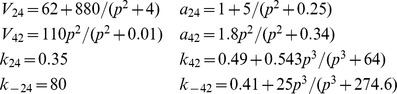Figure 9. Stationary data and fits of and .

Stationary transition rates of and , and , as functions of concentration were estimated and fitted for two , (A) and (B). Circles and squares represent the means of and distributions computed by MCMC simulation [7]. Note that MCMC failed to determine the values of and at for , as the was almost in the drive mode for these cases. The corresponding fitting curves (solid for ; dashed for ) are produced using Eqs. 7–12.

Figure 10. Open probability curves for various .

is equal to the sum of probabilities of the in and . Three representative curves correspond to , and (from bottom to top) respectively. Data (average open probability) are from [5].

Note that the above formulas are different from the relatively complicated formulas used in [8]. The rates, , and , are constants estimated by using dynamic single channel data [4] and given in Table 2, whereas is not clearly revealed by experimental data. However we have shown that it should be relatively large for high but relatively small for low for reproducing experimental puff data [8]. By introducing two concentrations, and , and the state of the channel become highly correlated, so that we can assume is a relatively large value if the channel is open and is a relatively small value if the channel is closed. Hence, is modeled by the logic function

Values of and are chosen so that simulated oscillations in ASMC are comparable to experimental observations.

The model reduction

Here we reduce the 6-state model to a 2-state open/closed model. The reduction takes the following steps:

• The sum of the probabilities of , and is less than 0.03 for any , so they are either rarely visited by the or have a very short dwell time. This implies they have very little contribution to the dynamics. Therefore, we completely remove the three states from the full model.

• Transition rates of and are about 2 orders larger than that of and , which allows us to omit the fast transitions by taking a quasi-steady state approximation. This change will affect two aspects. First, we have which allows us to combine and to be a new state , which satisfies . Although this means is a partially open state with an open probability of , it can be used as an fully open state in the stochastic simulations by multiplying the maximum flux conductance by a factor of . Secondly, needs to be rescaled by , i.e., the effective closing rate is .

• Due to the combination of and , is accordingly modified to

  

Hence, the reduced two-state model contains one “open” state and one closed state with the opening transition rate of and the closing transition rate of .

Deterministic formulation of the stochastic model

Based on the stochastic calcium model and the reduced 2-state model, we construct a deterministic model. We need to modify three things that are used in the stochastic model but inapplicable to fast simulations of the deterministic model. The first is the discrete number of open channels; the second is state-dependent use of and in calculating and ; the last is the logic expression of . Details of the modifications are as follows,

• The fraction of open channels () is replaced by open probability which is 70% of the probability of state .

• In the stochastic simulations, which only controls the closing is primarily governed by , whereas which controls opening is mainly governed by . Therefore, in the deterministic model, we separate the functions of and by assuming and are functions of only whereas and are functions of only. That is, , , and . Here as defined before.

• To describe an average rate that infinitely many receptors are rapidly inhibited by high concentration but slowly restored from -inhibition. is proposed to be

  

Based on the above changes, the full deterministic model containing 8 ODEs is presented as follows,

(13)

(14)

(15)

(16)

(17)

(18)

(19)

(20)

where and are functions of the gating variables given by Eqs. 4 and 5. All the fluxes are the same as those of the stochastic model except . All the parameter values of the deterministic model are the same as those of the stochastic model and are therefore given in Tables 1 and 2.

Reduction of the full deterministic model

The full deterministic model contains 8 variables which make the model difficult to implement and analyze. Thus, we reduce the full model to a minimal model that still captures the crucial features of the full model. First of all, , and are sufficiently large so that we can assume they instantaneously follow their equilibrium functions. Therefore, by taking quasi-steady state approximation to , and , we remove the three time-dependent variables from the full model.

By now, the full model has been reduced to a 5D model,

(21)

(22)

(23)

(24)

(25)

Second, the rate of change of approaching its equilibrium, (calculated from Eq. 24), is at least one order larger than those of , and , indicating that taking the quasi-steady state approximation to Eq. 24 could not significantly affect the evolutions of , and . That is,

(26)

We emphasize here that the theory of the quasi-steady state approximation has not yet been well established, particularly about the rigorous conditions under which such a reduction is valid. Thus, our criterion of judging the validity of the reduction is checking whether the solutions of the reduced model are capable of qualitatively reproducing that of its original model. For this model, we find the reduction works. Hence, the full model is eventually reduced to a 4D model summarized as follows,

(27)

(28)

(29)

(30)

where is given by Eq. 26.

Inclusion of calcium buffers

To check the effect of calcium buffers on oscillation frequency, we introduce a stationary buffer (no buffer diffusion), as mobile buffers are too complicated to be included in the current deterministic model. Since we have two different cytoplasmic concentrations, and , two pools of buffer with the same kinetics should be considered. Hence, the inclusion of a stationary calcium buffer is modeled by the following system,

(31)

(32)

(33)

(34)

(35)

where ( and ) and represent the concentrations of -bound buffer and total buffer respectively. and are the rates of -binding and -dissociation, indicating how fast the time scale of the buffer dynamics is. Fast buffer refers to the buffer with relatively large . In the simulations, we use a fast buffer with and and vary to test if the stochastic model and the deterministic model have a qualitatively similar -dependency. Results are given in Fig. 6E.

Numerical methods and tools for deterministic and stochastic simulations

For the stochastic model, Eqs. 1–3 and ODEs of the four gating variables in the model are solved by the fourth-order Runge-Kutta method (RK4) and the stochastic states of determined by the model are solved by using a hybrid Gillespie method with adaptive timing [37]. The maximum time step size is set to be either (for the 6-state model) or (for the reduced 2-state model). All the computations are done with MATLAB (The MathWorks, Natick, MA) and the codes are provided in Supporting information (Text S1–S2). For the deterministic model, we use ode15s, an ODE solver in MATLAB. Accuracy is controlled by setting an absolute tolerance of applied to all the variables.

Statistical analysis

Data analysis is performed on the traces with relatively stable baselines and less noise. A moving average of every 3 data points is used to improve the data by smoothing out short-term fluctuations (Fig. 2A is an improved result). Due to large variations in baseline, amplitude, and level of noise in data, we used two thresholds to get samples: a low threshold, 20% of the amplitude of the largest spike above the baseline, to initially filter baseline noise out; and a relatively high threshold, 50% of the amplitude of the largest spike above the baseline, to further remove small spikes that cannot initiate waves. For simulated stochastic traces of variable , we first convert it to fluorescence ratio () by using where the dissociation constant of Oregon Green and resting . We then used the same sampling procedure mentioned above to obtain samples. After samples are chosen, ISIs and spike durations are calculated based on the low threshold. Simulated traces used to calculate average frequency are about 200–400 seconds long. All the samplings and linear least-squares fittings are implemented using MATLAB (see Text S3–S4 for Matlab codes).

Supporting Information

Dataset S1

ASMC calcium fluorescence trace data. The data files are in Excel format and compressed in a zip file. Each Excel file has a name showing their information. For example, “S2_SMC6_MCh200nM” means data are from ASMC No. 6 in lung slice No. 2 by using 200 nM MCh. In each file, there are four columns which represent (from left to right) time(s), fluorescence intensity, and average .

(ZIP)

Text S1

Matlab code for simulation using 6 state model.

(DOCX)

Text S2

Matlab code for simulation using 2 state model.

(DOCX)

Text S3

Matlab code for experimental data analysis.

(DOCX)

Text S4

Matlab code for simulation analysis.

(DOCX)

Data Availability

The authors confirm that all data underlying the findings are fully available without restriction. All relevant data are within the paper and its Supporting Information files.

Funding Statement

Funding for all authors came from National Heart Lung Blood Institute (USA) RO1 HL103405. http://www.nhlbi.nih.gov/ The funders had no role in study design, data collection and analysis, decisions to publish, or preparation of the manuscript.

References

- 1. De Young GW, Keizer J (1992) A single-pool inositol 1, 4, 5-trisphosphate-receptor-based model for agonist-stimulated oscillations in Ca2+ concentration. Proc Natl Acad Sci USA 89: 9895–9899. [DOI] [PMC free article] [PubMed] [Google Scholar]
- 2. Dupont G, Goldbeter A (1993) One-pool model for Ca2+ oscillations involving Ca2+ and inositol 1,4,5-trisphosphate as co-agonists for Ca2+ release. Cell Calcium 14: 311–322. [DOI] [PubMed] [Google Scholar]
- 3. Atri A, Amundson J, Clapham D, Sneyd J (1993) A single-pool model for intracellular calcium oscillations and waves in the Xenopus laevis oocyte. Biophys J 65: 1727–1739. [DOI] [PMC free article] [PubMed] [Google Scholar]
- 4. Mak DOD, Pearson JE, Loong KPC, Datta S, Fernández-Mongil M, et al. (2007) Rapid ligand-regulated gating kinetics of single IP3R Ca2+ release channels. EMBO Rep 8: 1044–1051. [DOI] [PMC free article] [PubMed] [Google Scholar]
- 5. Wagner LE, Yule DI (2012) Differential regulation of the InsP3 receptor type-1 and -2 single channel properties by InsP3, Ca2+ and atp. J Physiol 590: 3245–3259. [DOI] [PMC free article] [PubMed] [Google Scholar]
- 6. Ullah G, Mak DOD, Pearson JE (2012) A data-driven model of a modal gated ion channel: the inositol 1,4,5-trisphosphate receptor in insect sf9 cells. J Gen Physiol 140: 159–173. [DOI] [PMC free article] [PubMed] [Google Scholar]
- 7. Siekmann I, Wagner LE, Yule DI, Crampin EJ, Sneyd J (2012) A kinetic model for IP3R type i and type ii accounting for mode changes. Biophys J 103: 658–668. [DOI] [PMC free article] [PubMed] [Google Scholar]
- 8. Cao P, Donovan G, Falcke M, Sneyd J (2013) A stochastic model of calcium puffs based on single-channel data. Biophys J 105: 1133–1142. [DOI] [PMC free article] [PubMed] [Google Scholar]
- 9. Smith IF, Parker I (2009) Imaging the quantal substructure of single IP3R channel activity during Ca2+ puffs in intact mammalian cells. Proc Natl Acad Sci USA 106: 6404–6409. [DOI] [PMC free article] [PubMed] [Google Scholar]
- 10. Brumen M, Fajmut A, Dobovišek A, Roux E (2005) Mathematical modelling of Ca2+ oscillations in airway smooth muscle cells. J Biol Phys 31: 515–524. [DOI] [PMC free article] [PubMed] [Google Scholar]
- 11. Sneyd J, Tsaneva-Atanasova K, Reznikov V, Bai Y, Sanderson MJ, et al. (2006) A method for determining the dependence of calcium oscillations on inositol trisphosphate oscillations. Proc Natl Acad Sci USA 103: 1675–1680. [DOI] [PMC free article] [PubMed] [Google Scholar]
- 12. Wang IY, Bai Y, Sanderson MJ, Sneyd J (2010) A mathematical analysis of agonist- and kcl-induced Ca2+ oscillations in mouse airway smooth muscle cells. Biophys J 98: 1170–1181. [DOI] [PMC free article] [PubMed] [Google Scholar]
- 13. Croisier H, Tan X, Perez-Zoghbi JF, Sandrson MJ, Sneyd J, et al. (2013) Activation of store-operated calcium entry in airway smooth muscle cells: insight from a mathematical model. PLoS ONE 8(7): e69598 10.1371/journal.pone.0069598 [DOI] [PMC free article] [PubMed] [Google Scholar]
- 14. Marchant JS, Parker I (2001) Role of elementary Ca2+ puffs in generating repetitive Ca2+ oscillations. EMBO J 20: 65–76. [DOI] [PMC free article] [PubMed] [Google Scholar]
- 15. Skupin A, Kettenmann H, Winkler U, Wartenberg M, Sauer H, et al. (2008) How does intracellular Ca2+ oscillate: by chance or by the clock? Biophys J 94: 2404–2411. [DOI] [PMC free article] [PubMed] [Google Scholar]
- 16. Perez JF, Sanderson MJ (2005) The frequency of calcium oscillations induced by 5-ht, ach, and kcl determine the contraction of smooth muscle cells of intrapulmonary bronchioles. J Gen Physiol 125: 535–553. [DOI] [PMC free article] [PubMed] [Google Scholar]
- 17. Bai Y, Edelmann M, Sanderson MJ (2009) The contribution of inositol 1,4,5-trisphosphate and ryanodine receptors to agonist-induced Ca2+ signaling of airway smooth muscle cells. Am J Physiol Lung Cell Mol Physiol 297: L347–L361. [DOI] [PMC free article] [PubMed] [Google Scholar]
- 18. Bird GSJ, Putney JW (2005) Capacitative calcium entry supports calcium oscillations in human embryonic kidney cells. J Physiol 562(3): 697–706. [DOI] [PMC free article] [PubMed] [Google Scholar]
- 19. Sneyd J, Tsaneva-Atanasova K, Yule DI, Thompson JL, Shuttleworth TJ (2004) Control of calcium oscillations by membrane fluxes. Proc Natl Acad Sci USA 101: 1392–1396. [DOI] [PMC free article] [PubMed] [Google Scholar]
- 20. Mahn K, Hirst SJ, Ying S, Holt MR, Lavender P, et al. (2009) Diminished sarco/endoplasmic reticulum Ca2+ atpase (serca) expression contributes to airway remodelling in bronchial asthma. Proc Natl Acad Sci USA 106: 10775–10780. [DOI] [PMC free article] [PubMed] [Google Scholar]
- 21. Sathish V, Leblebici F, Kip SN, Thompson MA, Pabelick CM, et al. (2008) Regulation of sarcoplasmic reticulum Ca2+ reuptake in porcine airway smooth muscle. Am J Physiol Lung Cell Mol Physiol 294: L787–L796. [DOI] [PubMed] [Google Scholar]
- 22. Zeller S, Rüdiger S, Engel H, Sneyd J, Warnecke G, et al. (2009) Modeling of the modulation by buffers of Ca2+ release through clusters of IP3 receptors. Biophys J 97: 992–1002. [DOI] [PMC free article] [PubMed] [Google Scholar]
- 23. Li Y, Rinzel J (1994) Equations for InsP3 receptor-mediated [Ca2+]i oscillations derived from a detailed kinetic model: a hodgkin-huxley like formalism. J Theor Biol 166: 461–473. [DOI] [PubMed] [Google Scholar]
- 24.Keener J, Sneyd J (2009) Mathematical Physiology, Second Edition. Springer, New York.
- 25. Ionescu L, White C, Cheung KH, Shuai J, Parker I, et al. (2007) Mode switching is the major mechanism of ligand regulation of InsP3 receptor calcium release channels. J Gen Physiol 130: 631–645. [DOI] [PMC free article] [PubMed] [Google Scholar]
- 26. Shuai JW, Jung P (2002) Stochastic properties of Ca2+ release of inositol 1,4,5-trisphosphate receptor clusters. Biophys J 83: 87–97. [DOI] [PMC free article] [PubMed] [Google Scholar]
- 27. Dupont G, Abou-Lovergne A, Combettes L (2008) Stochastic aspects of oscillatory Ca2+ dynamics in hepatocytes. Biophys J 95: 2193–2202. [DOI] [PMC free article] [PubMed] [Google Scholar]
- 28. Kannan MS, Prakash YS, Brenner T, Mickelson JR, Sieck GC (1997) Role of ryanodine receptor channels in Ca2+ oscillations of porcine tracheal smooth muscle. Am J Physiol 272: L659–L664. [DOI] [PubMed] [Google Scholar]
- 29. Tazzeo T, Zhang Y, Keshavjee S, Janssen LJ (2008) Ryanodine receptors decant internal Ca2+ store in human and bovine airway smooth muscle. Eur Respir J 32: 275–284. [DOI] [PubMed] [Google Scholar]
- 30. Ressmeyer AR, Bai Y, Delmotte P, Uy KF, Thistlethwate P, et al. (2010) Human airway contraction and formoterol-induced relaxation is determined by Ca2+ oscillations and Ca2+ sensitivity. Am J Respir Cell Mol Biol 43: 179–191. [DOI] [PMC free article] [PubMed] [Google Scholar]
- 31. Soeller C, Cannell MB (2004) Analysing cardiac excitation-contraction coupling with mathematical models of local control. Prog Biophys Mol Biol 85: 141–162. [DOI] [PubMed] [Google Scholar]
- 32. Thurley K, Skupin A, Thul R, Falcke M (2012) Fundamental properties of Ca2+ signals. Biochim Biophys Acta 1820(8): 1185–1194. [DOI] [PubMed] [Google Scholar]
- 33. Dickinson G, Parker I (2013) Factors determining the recruitment of inositol trisphosphate receptor channels during calcium puffs. Biophys J 105: 2474–2484. [DOI] [PMC free article] [PubMed] [Google Scholar]
- 34. Rüdiger S, Shuai JW, Sokolov IM (2010) Law of mass action, detailed balance, and the modeling of calcium puffs. Phys Rev Lett 105(4): 048103 10.1103/PhysRevLett.105.048103 [DOI] [PubMed] [Google Scholar]
- 35. Rüdiger S, Jung P, Shuai J (2012) Termination of Ca2+ release for clustered IP3R channels. PLoS Comput Biol 8(5): e1002485 10.1371/journal.pcbi.1002485 [DOI] [PMC free article] [PubMed] [Google Scholar]
- 36. Chandrasekera PC, Kargacim ME, Deans JP, Lytton J (2009) Determination of apparent calcium affinity for endogenously expressed human sarco(endo)plasmic reticulum calcium-atpase isoform serca3. Am J Physiol Cell Physiol 296: C1105–C1114. [DOI] [PubMed] [Google Scholar]
- 37. Rüdiger S, Shuai JW, Huisinga W, Nagaiah C, Warnecke G, et al. (2007) Hybrid stochastic and deterministic simulations of calcium blips. Biophys J 93: 1847–1857. [DOI] [PMC free article] [PubMed] [Google Scholar]
Associated Data
This section collects any data citations, data availability statements, or supplementary materials included in this article.
Supplementary Materials