PORTR: Pre-Operative and Post-Recurrence Brain Tumor Registration

Abstract

We propose a new method for deformable registration of pre-operative and post-recurrence brain MR scans of glioma patients. Performing this type of intra-subject registration is challenging as tumor, resection, recurrence, and edema cause large deformations, missing correspondences, and inconsistent intensity profiles between the scans. To address this challenging task, our method, called PORTR, explicitly accounts for pathological information. It segments tumor, resection cavity, and recurrence based on models specific to each scan. PORTR then uses the resulting maps to exclude pathological regions from the image-based correspondence term while simultaneously measuring the overlap between the aligned tumor and resection cavity. Embedded into a symmetric registration framework, we determine the optimal solution by taking advantage of both discrete and continuous search methods. We apply our method to scans of 24 glioma patients. Both quantitative and qualitative analysis of the results clearly show that our method is superior to other state-of-the-art approaches.

I. Introduction

The treatment of brain gliomas could greatly benefit from discovering imaging markers in the pre-operative scans that accurately predict tumor infiltration and subsequent tumor recurrence [1]-[3]. One possible approach for discovering these markers is to first align the pre-operative and the post-recurrence structural brain MR scans of a patient and then to analyze the imaging characteristics of tissue that later turn into tumor recurrence [4], [5]. This strategy relies on accurate registration as the size of tumor recurrence is usually not very large. However, nonrigid registration of the pre-operative and post-recurrence scans is very challenging due to large deformations, missing correspondences, and inconsistent intensity profiles between the scans. The large deformations and missing correspondences are due to the glioma in the pre-operative scans causing large mass effects [6] as well as the resection cavities and tumor recurrence in the post-recurrence scans, which are acquired several months or years after surgery. The inconsistent intensity profiles result from tissue labeled as edema in the pre-operative scan transforming to healthy tissue in the post-recurrence scan (and vice versa). Thus, corresponding regions can have very different intensity profiles. Fig. 1 shows a typical case with the anatomy around the tumor being confounded by resection cavity, tumor recurrences, and edema. In this paper, we develop a registration method to cope with the missing correspondence issue between the scans and show that the results are much more accurate than general-purpose registration methods.

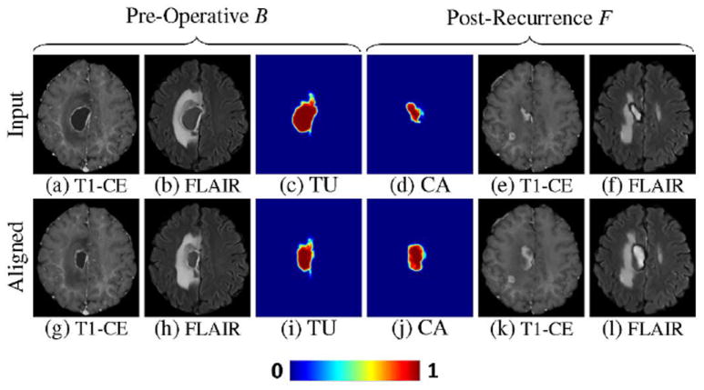
Fig. 1.

Example of the pre-operative scan B and the corresponding post-recurrence scan F. Pre-operative scan B clearly shows the tumor in the T1-CE scan and edema in FLAIR scan. Edema is also clearly visible in the FLAIR scan of the post-recurrence scan F. T1-CE of F now shows resection cavity and tumor recurrence.

Existing registration methods mostly deal with the missing correspondence issue by excluding the pathology during the mapping process [7]-[9]. They require segmentations of the brain scans, such as Clatz et al. [10], who align the pre-operative and intra-operative brain scans by first matching selected regions of healthy tissue. The approach then applies a bio-mechanical model to the resulting map to interpolate the deformations to the remaining image domain. Risholm et al. [11] avoid the prerequisite of a label map by alternating between extracting the resection area and estimating deformations. However, it is difficult to estimate gross deformation on brain glioma scans by excluding the pathology. To take explicit account of the tumor region, approaches register tumor scans to a healthy brain template by simulating mass effects of the tumor on the template [12], [13]. Alternatively, generative models, such as Prastawa et al. [14] and Menze et al. [15], inject a prior of the tumor into an atlas of a healthy population and segment the tumor by aligning this atlas to the scan. Gooya et al. [16] extend this idea to nonrigid registration by growing the tumor inside the atlas until the deformed atlas resembles the pathology and healthy tissue shown in the brain tumor scan.

To the best of our knowledge, this paper proposes the first approach specifically targeted towards the registration of pre-operative and post-recurrence glioma scans, called Pre-Operative and post-Recurrence brain Tumor Registration (PORTR). One could register an atlas to each scan individually, for example via [16], and then concatenate the corresponding registrations [17]. However, this approach ignores the fact that the scans are from the same patient. It thus has to solve the much more difficult problem of registering an atlas of a healthy population to scans showing pathology. Alternatively, one can directly register the scans using state-of-the-art intensity- or feature-based registration methods [18]-[20]. However, these approaches do not explicitly account for pathologies and therefore may produce unreasonable correspondences in these areas. PORTR instead makes use of the fact that both scans are from the same patient and explicitly models constraints enforced by the pathology in each scan.

PORTR determines the optimal deformation between two scans by finding the minimum of an energy function, which is based on the concept of symmetric registration [19], [21]-[24]. This energy function is not only comprised of image-based correspondences and smoothness constraints as customary for other registration methods, but also includes pathological information. The pathological information is inferred from the results of two segmenters that are targeted to each scan. Specifically, we develop a new method for segmenting post-recurrence scans, which generally consist of resection cavities after brain surgery and multiple tumor recurrences. For the pre-operative scans, we adapt the segmenter by Gooya et al. [16] to outline a single brain glioma which causes a large mass effect on healthy tissue. The resulting segmentations of both scans are a central component in the definition of the image and the shape-based correspondence terms within our symmetric registration framework. Determining the minimum within this framework is difficult as the function contains many local minima. We deal with these difficulties by combining discrete and continuous optimizations. The discrete optimization method finds the optimal solution in a coarse solution space. The continuous optimization method locally improves this solution in a finer solution space. We measure the accuracy of PORTR on 24 subjects. The results indicate that the proposed method outperforms Avants et al. [19] and Ou et al. [20], two examples of the state-of-the-art in general-purpose registration methods.

II. Deformable Registration Framework For Tumor Scans

We now describe PORTR, which aligns the pre-operative scan (baseline, denoted as B) with the post-recurrence scan (follow-up, denoted as F) of the same subject. As outlined in Fig. 2, our approach first applies atlas-based segmenters to F (Step 1) and B (Step 2) to extract pathological information needed to register the scans (Step 3). Our analysis starts with F instead of B as the glioma shown in B is surgically removed in F. Thus, the healthy tissue of F is not impacted by the large mass effect of that glioma [25], [26] so that segmenters guided by atlases of healthy populations are generally easier adapted to F than B. We do so in Step 1 by exploring a new multi-tumor model for modifying the atlas of the healthy population to scan F. We then interpret the results of Step 1 as a scan-specific atlas for Step 2 guiding the joint atlas registration and segmentation of the pre-operative scan B [16]. The registration of Step 2 initializes the registration between and F of Step 3. For Step 3, we propose a new probabilistic registration framework coupling the results of the previous steps with the image-based correspondences between F and B.

Fig. 2.

Our deformable registration framework consists of three steps. We first create a scan-specific atlas for F by segmenting the scan (Step 1). We then jointly register this atlas to B and segment the scan, which provides an initial mapping between F and B (Step 2). Finally, we register the scans using the results from the previous two steps (Step 3).

A. Step 1: Segmentation of Post-Recurrence Scan

The goal of this step is to compute probabilities regarding the presence of healthy tissue and pathology within the post-recurrence scan F. We do so by simultaneously registering an atlas to scan F and segmenting the anatomy in that scan. The atlas provides spatial information about the structures of interest, which is needed to distinguish between the similar MR intensity patterns of healthy tissue and pathology. In the remainder of this section, we first provide a simple model for transforming an atlas of a healthy population to one including pathological information specific to scan F. We then integrate the atlas into our Bayesian approach for joint segmentation and registration of the post-recurrence scan.

Before describing our probabilistic model in further detail, we introduce the following nomenclature: Τ denotes the label map across the image Ω_F domain of scan F. The possible label t of Τ at a specific location x ∈ Ω_F is WM (white matter), GM (gray matter), CSF (cerebrospinal fluid), ED (edema), and TU (tumor), which includes enhanced tumor, necrosis and cavity. For short, we denote this as “Τ_t | x” instead of “Τ = t | x.” p_A is the probabilistic brain tissue atlas of a healthy population, which we assume to be affinely aligned with F. Let Θ_A ≜ {WM, GM, CSE} be the labels of the healthy tissue types then p_A(Τ_t | x) is the probability of tissue t ∈ Θ_A being present at location x ∈ Ω_F [see Fig. 3(c)–(e)]. Similarly, p_F corresponds to the probabilistic model associated with scan F, Θ ≜ {WM, GM, CSF, ED, TU} are the labels of all possible tissue types on p_F, and the spatial probability p_F(Τ_t | x) is the conditional probability of tissue t ∈ Θ being present at location x ∈ Ω_F.

Fig. 3.

Atlas created by Step 1. Figure shows the post-recurrence scan F in (a) and (b), and a probabilistic atlas of a healthy population in (c)–(e). Images (f)–(j) are the spatial probabilities p_F(Τ_t) based on our multi-tumor model applied to the healthy atlas. Images (k)–(o) shows the spatial probabilities aligned to the scan. Those spatial distributions better fit to the scan than the original ones (f)–(j).

We now define p_F(Τ_t | x) for each t ∈ Θ by combining p_A with a simple model for pathology. This model is based on the empirical observation that the post-recurrence scan F generally shows multiple small tumor recurrences, resection cavities, and edema. These pathologies do not cause a large mass effect on the healthy tissue in general. Our spatial probabilities p_F(Τ_t | x) are therefore based on the simplifying assumptions that the mass effect of the pathologies on healthy tissue can be ignored and that each pathological region is contained within a relatively small sphere. If we assume F shows M tumors then each tumor i ∈ {1, … M}, which we loosely use for tumor recurrences and resection cavities, can thus be characterized by its center location o_i ∈ Ω_F and its size or radius r_i. We manually set o_i and r_i so that the resulting sphere encompasses the abnormal region as shown on T1-CE scans. Based on the previous assumptions, we model its corresponding spatial probability via the generalized logistic function [27]

$$\mathit{Y}(\mathbf{x},{\mathbf{o}}_i,r_i,a)\triangleq \frac{1}{1+\exp \{a\cdot (\parallel \mathbf{x}-{\mathbf{o}}_i\parallel -r_i)\}}$$ (1)

where ‖ · ‖ is the ℓ²-norm and a controls the steepness of the function. Fig. 4 plots the radial profile for (1) with different parameters. The graph shows that the curves start to slope further away from the origin as r_i gets larger and their slope steepens as a gets larger. This slope represents the diffusion of the tumor into healthy tissue. For simplicity, we set a = a_TU uniformly across all tumors. The spatial probability p_F(Τ_TU | x) across all tumors is then defined by the maximum value of the M individual spatial probabilities Y as follows:

$$p_F\left({{\rm T}}_{\mathrm{TU}}|\mathbf{x}\right)\triangleq \underset{i}{\max }\left\{Y\left(\mathbf{x},{\mathbf{o}}_i,r_i,a_{\mathrm{TU}}\right)\right\}.$$ (2)

Fig. 4.

Radial profiles of spatial probability functions Y with varying parameters. As Y is radially symmetric, we set the x-axis as the distance from the tumor center (o_i is located at zero). Four sample curves for Y are based on different parameter settings for r_i ∈ {15, 30, 45, 60} and a ∈ {0.8, 0.6, 0.4, 0.2}. Plot in blue is an edema model combining graphs labeled as Y₁ and Y₂. Graphs show the curves start to slope further away from the origin the larger r_i is and their slope steepen the larger a is.

We use the maximum across the spatial distributions of all tumors as the function preserves the probabilistic profile of individual tumors (assuming they are well spaced) and ensures the range of p_F(Τ_TU | x) to be within [0,1].

The spatial probability of edema is based on the assumption that edema is in close proximity of tumors and its signal strength decays smoothly as the distance from the tumor center increases. Furthermore, edema is contained inside white matter and should be defined in relation to tumor. In other words, the more probable the presence of tumor, the less probable edema should be. These assumptions are summarized in the following definition of the spatial probability of edema:

$$\begin{array}{r}\hfill p_F({{\rm T}}_{\mathrm{ED}}|\mathbf{x})\triangleq 0.5\cdot p_A({{\rm T}}_{\mathrm{WM}}|\mathbf{x})\cdot (1-p_F({{\rm T}}_{\mathrm{TU}}|\mathbf{x}))\\ \hfill \cdot \underset{i}{\max }\{Y(\mathbf{x},{\mathbf{o}}_i,b_{\mathrm{ED}}\cdot r_i,a_{\mathrm{ED}})\}.\end{array}$$ (3)

We set a_ED < a_TU, which means edema is more dispersed than tumor. b_ED defines the area of edema with respect to the ith pathological region. Also, the factor 0.5 ensures that our atlas does not favor edema over WM (or vice versa) in areas of Y ≈ 1 in (3). Fig. 4 shows the radial profile for p_F(Τ_TU | x) (red line) and p_F(Τ_ED | x) (blue line) assuming a single tumor is present and its size is r_i = 15. One can see that the probability of edema is close to zero inside the tumor, increases to 0.5, and then it smoothly decays to zero again.

Next, we model the spatial probabilities of the healthy tissue classes. We combine the atlas p_A with p_F (Τ_TU | x) based on the observation that in areas where p_F(Τ_TU | x) is relatively large, the probability of healthy tissue should be small. For GM and CSF, this observation is reflected by the following product(t ∈ {GM, CSF}):

$$p_F\left({{\rm T}}_t|\mathbf{x}\right)\triangleq p_A\left({{\rm T}}_t|\mathbf{x}\right)\cdot \left(1-p_F\left({{\rm T}}_{\mathrm{TU}}|\mathbf{x}\right)\right).$$

For WM, we take the complement of spatial probabilities of the other labels

$$\begin{array}{cc}{p}_F({{\rm T}}_{\mathrm{WM}}|\mathbf{x})\triangleq & 1-\{p_F({{\rm T}}_{\mathrm{TU}}|\mathbf{x})+p_F({{\rm T}}_{\mathrm{ED}}|\mathbf{x})\\ & \hfill +p_F({{\rm T}}_{\mathrm{GM}}|\mathbf{x})+p_F({{\rm T}}_{\mathrm{CSF}}|\mathbf{x})\}.\end{array}$$

Note that p_F(Τ_WM | x) is always nonnegative. Fig. 3(f)–(j) shows an example of our spatial probabilities. The spatial probability for edema is high in close proximity of tumors. Furthermore, spatial probabilities for WM, GM, and CSF are decreased in comparison to their values in the healthy atlas in areas where tumor or edema appears to be present.

Having defined the spatial probabilities p_F(Τ_t | x), we now describe our approach for computing the posterior probabilities of all tissue types. For p_F(Τ_t | x) to be informative it needs to match F. Fig. 3(f)–(j) shows that this is generally not the case. For example, p_F(Τ_t | x) implies a high probability of tumor outside the pathology shown in F. We address this issue by jointly computing posterior probabilities and registering p_F(Τ_t | x) to F.

One of the parameters of our joint registration and segmentation model is h_F, the “voxel wise mapping” from the Ω_F to the atlas space. A voxel-wise mapping projects a voxel from the source to target space according to the 3-D vector stored in the underlying deformation map at that location. The second set of parameters are the tissue specific mean and covariances Ф_F, which define the multivariate Gaussian of the image likelihood p_F(F | Τ_t, Ф_F, x). The joint registration and segmentation problem is then defined via the following optimization problem:

$$\begin{array}{r}\hfill \{{\mathit{h}}_F^{\ast },{\mathbf{\Phi }}_F^{\ast }\}\triangleq \arg \underset{{\mathit{h}}_F,{\mathbf{\Phi }}_F}{\max }(\prod _{\mathbf{x}\in {\mathrm{\Omega }}_F}\sum _{t\in \mathrm{\Theta }}{p}_F({{\rm T}}_t|{\mathit{h}}_F(\mathbf{x}))\\ \hfill \cdot p_F(F|{{\rm T}}_t,{\mathbf{\Phi }}_F,\mathbf{x})).\end{array}$$ (4)

We obtain ${\mathit{h}}_F^{\ast }$ and ${\mathbf{\Phi }}_F^{\ast }$ via an implementation of the expectation-maximization (EM) algorithm [28]. The details of this implementation are provided in Appendix A. Then we define the posteriors for the post-recurrences scan with respect to the anatomy t ∈ Θ as

$$\begin{array}{ll}{p}_F({{\rm T}}_t|F,\mathbf{x})& \triangleq p_F({{\rm T}}_t|F,{\mathit{h}}_F^{\ast },{\mathbf{\Phi }}_F^{\ast },\mathbf{x})\\ & \mathrm{\propto }{p}_F({{\rm T}}_t|{\mathit{h}}_F^{\ast }(\mathbf{x}))\cdot p_F(F|{{\rm T}}_t,{\mathbf{\Phi }}_F^{\ast },\mathbf{x}).\end{array}$$ (5)

Fig. 3(k)–(o) shows the aligned spatial probability $p_F({{\rm T}}_t|{\mathit{h}}_F^{\ast }(\mathbf{x}))$ obtained by applying ${\mathit{h}}_F^{\ast }$ to the original spatial probability p_F(Τ_t | x) of Fig. 3(f)–(j). The probability for each tissue is transformed to match the scan. The aligned spatial probability of tumor (k) correlates now very well with the scan compared to its original (f).

B. Step 2: Segmentation of Pre-Operative Scan

The goal of this step is to segment pathological regions from the pre-operative scan B and to provide a rough estimation of the deformation between F and B. We achieve this goal via the joint segmentation and registration approach by Gooya et al. [16], called GLISTR. GLISTR explicitly models the generally large mass effects on healthy tissue caused by brain glioma in scan B. We now describe the integration of the results of Step 1 into this approach and provide a brief review of the method.

Similar to Step 1, GLISTR uses the EM algorithm to jointly register an atlas to the scan B and segment the scan B into healthy tissue and pathological regions. For our specific application, we replace the atlas of a healthy population proposed in [16] with the scan-specific atlas defined for tissue t ∈ Θ _A as

$$p_S\left({{\rm T}}_t|\mathbf{x}\right)\triangleq p_A({{\rm T}}_t|{\mathit{h}}_F^{\ast }\left(\mathbf{x}\right))$$ (6)

where the mapping ${\mathit{h}}_F^{\ast }$ was defined according to (4) in Step 1. Fig. 5(c)–(e) shows an example of the scan-specific atlas. This atlas is not affected by pathology and is aligned with F [see Fig. 3(a) and (b)].

Fig. 5.

Example of spatial probabilities in Step 2. We show the pre-operative scan B in (a) and (b) and scan-specific atlas in (c)–(e). In (f)–(j), we show spatial probabilities p_B(Τ_t) obtained by applying the tumor growth model on scan-specific atlas. (k)–(o) shows the spatial probabilities aligned to the scan. This atlas now fits well to healthy tissue and pathological regions shown in (a) and (b).

By registering this atlas to scan B, the method also approximates the mapping between F and B. We note that we could have also based the atlas on the posteriors of (5) instead of $p_A({{\rm T}}_t|{\mathit{h}}_F^{\ast }(\mathbf{x}))$. Compared to $p_A({{\rm T}}_t|{\mathit{h}}_F^{\ast }(\mathbf{x}))$, the posteriors have generally higher certainty about the presence or absence of healthy tissue throughout the image domain. The higher certainty causes the method to have less flexibility in registering p_S to B. In practice, this makes the registration problem more difficult causing the method to be less stable than when using our proposed atlas.

The remainder of this section provides a brief overview of how GLISTR simultaneously models tumor growth in the atlas space, registers the corresponding atlas to scan B, and segments B. We denote with p_B the probabilistic model specific to the scan B and Ω_B as the space of the pre-operative scan. As in the previous step, Τ represents the label map that at each image location is assigned to the labels of Θ. The approach adapts p_S to B by simulating tumor growth on Ω_F via the diffusion-reaction-advection model by Hogea et al. [29]. Given the parameters q, which contain the seed location of the tumor, the model produces the tumor probability p_B(Τ_TU | q, x) and the voxel-wise mapping u according to this tumor probability. We manually set the seed in the center of the tumor. The approach then combines p_B(Τ_TU | q, x) and u with the atlas p_S. Now, the spatial probabilities for GM and CSF (t ∈ {GM, CSE}) are defined as

$$p_B\left({{\rm T}}_t|\mathbf{q},\mathbf{x}\right)\triangleq p_S\left({{\rm T}}_t|\mathbf{u}\left(\mathbf{x}\right)\right)\cdot \left(1-p_B\left({{\rm T}}_{\mathrm{TU}}|\mathbf{q},\mathbf{x}\right)\right).$$ (7)

Unlike thein Step 1 (3), GLISTR models the close proximity of edema to tumor via the Heaviside function H(·), (H(a) = 0 for a ≤ 0 and H(a) = 1 for a > 0) resulting in

$$\begin{array}{r}{p}_B({{\rm T}}_{\mathrm{ED}}|\mathbf{q},\mathbf{x})\triangleq 0.5\cdot p_S({{\rm T}}_{\mathrm{WM}}|\mathbf{u}(\mathbf{x}))\cdot (1-p_B({{\rm T}}_{\mathrm{TU}}|\mathbf{q},\mathbf{x}))\\ \hfill \cdot H(p_B({{\rm T}}_{\mathrm{TU}}|\mathbf{q},\mathbf{x}))\end{array}$$ (8)

where we multiply 0.5 in order to avoid preference of edema over WM (or vice versa) as in (3). The Heaviside function explicitly confines edema to the region inferred from the outcome of the tumor growth model represented by p_B(Τ_TU | q, x). This region generally encompasses edema as the tumor growth model accounts for diffusion into healthy tissue. Note that Step 1 did not include a dynamic tumor model. We instead modeled diffusion through the logistic function with a fixed slope (1), which we then used to define the edema region. The spatial probability for WM is defined by the complement of spatial probabilities of the other labels

$$\begin{array}{cc}{p}_B({{\rm T}}_{\mathrm{WM}}|\mathbf{q},\mathbf{x})\hfill & \triangleq 1-\{p_B({{\rm T}}_{\mathrm{TU}}|\mathbf{q},\mathbf{x})+p_B({{\rm T}}_{\mathrm{ED}}|\mathbf{q},\mathbf{x})\\ & \hfill +p_B({{\rm T}}_{\mathrm{GM}}|\mathbf{q},\mathbf{x})+p_B({{\rm T}}_{\mathrm{CSF}}|\mathbf{q},\mathbf{x})\}.\end{array}$$

The EM algorithm determines the optimal parameters of this model, which are the tumor parameters q*, the voxel-wise mapping ${\mathit{h}}_B^{\ast }$ of the posteriors of B to the scan-specific atlas, and the Gaussian intensity distribution parameters ${\mathbf{\Phi }}_B^{\ast }$. The posterior of structure t ∈ Θ for the pre-operative scan B is then defined as

$$\begin{array}{ll}{p}_B({{\rm T}}_t|B,\mathbf{x})& \triangleq p_B({{\rm T}}_t|B,{\mathbf{q}}^{\ast },{\mathit{h}}_B^{\ast },{\mathbf{\Phi }}_B^{\ast },\mathbf{x})\\ & \mathrm{\propto }{p}_B({{\rm T}}_t|{\mathbf{q}}^{\ast },{\mathit{h}}_B^{\ast }(\mathbf{x}))\cdot p_B(B|{{\rm T}}_t,{\mathbf{\Phi }}_B^{\ast },\mathbf{x}).\end{array}$$ (9)

Let u* represent the mapping according to the tumor growth model, which is parameterized by q*. We approximate the mapping between scan B and F by concatenating “ο” two mappings ${\mathit{h}}_B^{\ast }$ and u*

$${\mathit{f}}_{BF}^0\triangleq {\mathbf{u}}^{\ast }\circ {\mathit{h}}_B^{\ast }.$$ (10)

Note that the voxel-wise mapping ${\mathit{f}}_{BF}^0$ approximates the alignment from B to F as we use p_S instead of image and pathological information for F.

Fig. 5(f)–(j) shows an example of spatial probabilities p_B(Τ_t | x). The spatial probability of tumor (f) covers the tumor shown in (a) and (b), the one of edema (g) is neighboring the tumor, and probabilities of healthy tissues are displaced by mass effect of the tumor. Fig. 5(k)–(o) shows aligned spatial probabilities $p_B({{\rm T}}_t|{\mathit{h}}_B^{\ast }(\mathbf{x}))$ which better seem to fit the scan than those of Fig. 5(f)–(j).

C. Step 3: Deformable Registration of Pre-Operative and Post-Recurrence Scans

The goal is now to register the pre-operative scan B and the post-recurrence scan F to accurately match the intensities of the nonpathological regions while simultaneously inferring reasonable deformations for the pathology based on the posterior probabilities of the previous two steps. We do so by applying the concept of symmetric registration [19], [21]-[24] to our scenario. The idea behind the symmetric registration is not to favor either scan by matching both scans to a “center coordinate system.” The mapping between the two scans is now essentially split into two. This splitting allows us to reliably determine the large deformations between the scans. To determine the optimal mapping, we apply a hybrid optimization method combining discrete and continuous optimizations. It allows us to refine the global solution of the coarse search space determined by the discrete optimization with the local search by the continuous optimization.

1) Symmetric Registration Framework

Let Ω_C be the center coordinate system, f_CB : Ω_C → Ω_B the diffeomorphic mapping from Ω_C to Ω_B, f_CF : Ω_C → Ω_F the diffeomorphic mapping from Ω_C to Ω_F, and “ο” concatenates two mappings. Then

$${\mathit{f}}_{\mathit{BF}}\triangleq {\mathit{f}}_{CF}\circ {({\mathit{f}}_{\mathit{CB}})}^{-1}$$ (11)

maps B to F. The solution to our symmetric registration problem $\{{\mathit{f}}_{\mathit{CB}}^{\ast },{\mathit{f}}_{\mathit{CF}}^{\ast }\}$ minimizes an energy function E(·)

$$\{{\mathit{f}}_{\mathit{CB}}^{\ast },{\mathit{f}}_{\mathit{CF}}^{\ast }\}=\arg \underset{{\mathit{f}}_{\mathit{CB}},{\mathit{f}}_{\mathit{CF}}}{\min }E({\mathit{f}}_{\mathit{CB}},{\mathit{f}}_{\mathit{CF}};B,F,p_B,p_F).$$ (12)

E(·) encodes the relationship between Ω_C, Ω_B and Ω_F by a correspondence term E_C measuring the agreement between image patches of B and F, a pathology term E_P capturing the overlap between posteriors of tumors in both scans, and a smoothness term E_S enforcing consistency across the deformation fields. Thus, the energy function is of the form

$$\begin{array}{l}E({\mathit{f}}_{\mathrm{CB}},{\mathit{f}}_{\mathrm{CF}};B,F,p_B,p_F)\\ \triangleq {\lambda }_D\cdot E_C({\mathit{f}}_{\mathrm{CB}},{\mathit{f}}_{\mathrm{CF}};B,F,p_B,p_F)\\ +{\lambda }_D\cdot {\lambda }_P\cdot E_P({\mathit{f}}_{\mathrm{CB}},{\mathit{f}}_{\mathrm{CF}};p_B,p_F)\\ +E_S({\mathit{f}}_{\mathrm{CB}},{\mathit{f}}_{\mathrm{CF}})\end{array}$$ (13)

where λ_D is a weight of data terms (E_C and E_P) compared to E_S and λ_P is a weight of E_P among data terms. The remainder of this section describes the three terms in further detail.

The correspondence term E_C is based on normalized cross-correlation (NCC) [30] to measures the image similarity of healthy tissue between the aligned baseline scan B ∘ f_CB and follow-up scan F ∘ f_CB in Ω_C. We choose NCC as it is often used for intra-subject registrations [18]. In our case, each scan consists of N co-registered, multi-modal images (e.g., T1, T1-CE, T2, and FLAIR) and B_i (or F_i) denotes the ith image of B (or F). The NCC of these multi-modal images at voxel x ∈ Ω_C is the mean NCC score across the modalities

$$D_{\mathrm{NCC}}(B\circ {\mathit{f}}_{CB},F\circ {\mathit{f}}_{CF},\mathbf{x})\triangleq \frac{1}{N}\sum _{i=1}^N\frac{\langle \overline{B_i},{\overline{F}}_i\rangle }{\sqrt{\langle \overline{B_i},\overline{B_i}\rangle \cdot \langle \overline{F_i},\overline{F_i}\rangle }}$$ (14)

with 〈·, ·〉 being the inner product of aligned and intensity-corrected patches $\overline{B_i}$ and $\overline{F_i}$. To compute $\overline{B_i}$ and $\overline{F_i}$, we define the region of the patch R(x) ⊂ Ω_C centered around x and compute the mean intensity value m(x) for that patch. Then

$$\overline{I_i}\triangleq \{I_i({\mathit{f}}_{CI}(\mathbf{y}))-m(\mathbf{x})|\mathbf{y}\in R(\mathbf{x})\}$$

for each I ∈ {B, F}. To confine the correspondence term E_C(·) to healthy tissue, we incorporate the probability for pathological regions in this term. As the pathology is indicated by tumor and edema, the probability for pathological regions p_I,_PT in each scan I ∈ {B, F} is defined as the sum of the posteriors of tumor and edema, i.e.,

$$p_{I,\mathrm{PT}}\left(\mathbf{x}\right)\triangleq p_I({{\rm T}}_{\mathrm{TU}}|I,\mathbf{x})+p_I({{\rm T}}_{\mathrm{ED}}|I,\mathbf{x}).$$

As shown in Fig. 6(e) and (j), p_B,_PT and p_F,_PT are good indicators for pathology. Now we know that pathology creates image patterns that are scan specific and thus unreliable for image matching. The opposite is true for healthy tissue. One way to reflect this observation in E_C is to use these probabilities as saliency information weighing D_NCC more in healthy regions and less in pathological regions. The following definition of the correspondence terms does exactly that:

$$\begin{array}{c}{E}_C({\mathit{f}}_{CB},{\mathit{f}}_{CF};B,F,p_B,p_F)\\ \triangleq {\mathit{\int }}_{\mathbf{x}\in {\mathrm{\Omega }}_C}\{1-p_{B,\mathrm{PT}}({\mathit{f}}_{CB}(\mathbf{x}))\}\cdot \{1-p_{F,\mathrm{PT}}({\mathit{f}}_{CF}(\mathbf{x}))\}\\ \cdot D_{\mathrm{NCC}}(B\circ f_{CB},F\circ f_{CF},\mathbf{x})d\mathbf{x}.\end{array}$$ (15)

Fig. 6.

Example of posteriors estimated by Step 1 and 2. For the pre-operative scan B shown in (a) and (b), the posteriors of (c) tumor and (d) edema are obtained by Step 2. For the post-recurrence scan F shown in (f) and (g), posteriors of (h) tumor and (i) edema are obtained by Step 1. In (h), the yellow arrow marks the regions for cavity and the red arrow marks the region for tumor recurrence. The probabilities for pathological regions (e) p_B,_PT and (j) p_F,_PT are defined as the sum of the posteriors of tumor and edema. In (e) and (j), the regions indicating high probability of tumor being present are matched well with pathological regions in B and F, respectively. Thus, those two maps are well suited for masking out pathological regions in the matching cost function.

The pathology term E_P measures the overlap between the tumor in B and the resection cavity in F. Similar to E_C, we use the posterior of tumor of Step 2 to indicate the tumor region in B. To flag the cavity region in F, we separate the seeds used for the posterior of tumor of Step 1 in those that are associated with cavities versus those with tumor recurrences. We then set the indicator variable 1_CA(x) at voxel x ∈ Ω_F to one if the index i(x) = arg max_i{Y(x, o_i, r_i, a)} used in (2) corresponds to seeds for the cavity, and otherwise set to zero. Then the posterior probability of cavity is

$$p_{F,\mathrm{CA}}(\mathbf{x})\triangleq p_F({{\rm T}}_{\mathrm{TU}}|F,\mathbf{x})\cdot {\mathbf{1}}_{\mathrm{CA}}({\mathit{h}}_F^{\ast }(\mathbf{x})).$$ (16)

Fig. 7(d) shows an example of p_F,_CA obtained from Fig. 6(h) using (16). Only the cavity region of Fig. 6(h) is correctly selected in Fig. 7(d).

Fig. 7.

Example of scans and posteriors aligned by Step 3. The upper row shows input scans and their estimated posteriors of (c) tumor and (d) cavity. Posterior of cavity (d) is obtained from the posterior of tumor shown in Fig. 6(h) using (16). Lower row shows the aligned scans and posteriors. Specifically, (g)–(i) are warped from (a)–(c) using and ${\mathit{f}}_{CB}^{\ast }$ (j)–(l) are warped from (d)–(f) using ${\mathit{f}}_{CF}^{\ast }$. Now the tumor nicely matches the cavity region.

We now define the pathology term E_P in such a way that it penalizes mismatches between the aligned posteriors of the tumor in B and of the cavity in F, i.e., we measure the squared ℓ²-norm between the aligned p_B,_TU and p_F,_CA [31], [32]

$$\begin{array}{c}{E}_P({\mathit{f}}_{\mathit{CB}},{\mathit{f}}_{\mathit{CF}};p_B,p_F)\\ \triangleq {\mathit{\int }}_{\mathbf{x}\in {\mathrm{\Omega }}_C}{\{p_{B,\mathrm{TU}}({\mathit{f}}_{\mathit{CB}}(\mathbf{x}))-p_{F,\mathrm{CA}}({\mathit{f}}_{\mathit{CF}}(\mathbf{x}))\}}^{2}d\mathbf{x}.\end{array}$$ (17)

In our experiments, this term performed slightly better than information theoretic measures such as the Jensen–Shannon (JS) divergence [33]. This is not surprising for shape alignment according to Wang et al. [34]. More importantly, the above term is more efficient to compute than JS. During optimizations, E_P leads tumor and cavity regions to correspond to each other which is difficult to do based on image-based correspondences. Fig. 7(c) and (d) shows the tumor and cavity posteriors, and Fig. 7(i) and (j) shows the corresponding regions with (c) and (d) transformed to have similar shapes after optimizations.

The third and final term of E(·) is the smoothness term E_S, which penalizes discontinuities in both f_CB and f_CF. measures the smoothness of the mappings f_CB and f_CF via the Tikhonov operator L [35]-[37]. Let c_i be a nonnegative constant and Id(x) = x be the identity mapping, then the Tikhonov operator of a mapping f is

$$L\mathit{f}\triangleq \sum _{i=0}^{\infty }{c}_i\cdot {\left|{\nabla }^i(\mathit{f}-\mathrm{Id})\right|}^2$$ (18)

where ∇ⁱ(f – Id) is the ith order derivative of the displacement field (f – Id). The smoothness term is now defined as

$$E_S({\mathit{f}}_{\mathit{CB}},{\mathit{f}}_{\mathit{CF}})\triangleq {\mathit{\int }}_{\mathbf{x}\in {\mathrm{\Omega }}_C}\{L{\mathit{f}}_{\mathit{CB}}(\mathbf{x})+L{\mathit{f}}_{\mathit{CF}}(\mathbf{x})\}d\mathbf{x}.$$ (19)

Algorithm 1. Our hybrid optimization method. We initialize the solution using ${\mathit{f}}_{BF}^0$ and then update the mappings {f_CB, f_CF} from coarse to fine scales sequentially executing discrete and continuous optimizations for each image resolution.

This regularizer favors smooth deformations as it penalizes magnitude of higher order derivatives [36]. We note that our method is not specific to the Tikhonov operator so that any other operator penalizing discontinuities in the displacement field could be used at this point.

This completes our definition of the energy function E, whose minimum [see (12)] defines our solution for determining the mappings f_CB and f_CF.

2) Hybrid Optimization Method

We determine the minimum of (12) via a hybrid approach combining discrete with continuous optimization, a concept recently explored in optical flow estimations [38], [39]. Discrete optimizations generally determine the global minimum (or a strong local minimum) but do so with respect to a limited search space. On the other hand, continuous optimization methods search in a much richer solution space but often get trapped in local minima causing them to be sensitive towards their initialization. To take advantage of both approaches, we first apply our discrete optimization method and use those results as initialization of the continuous optimization method.

As outlined in Algorithm 1, we initialize our algorithm by “splitting” the initial displacement ${\mathit{f}}_{BF}^0$ of (10) in half

$$\begin{array}{l}{\mathit{f}}_{\mathit{CB}}\leftarrow {\left(\mathrm{Id}+\frac{{\mathit{f}}_{\mathit{BF}}^0-\mathrm{Id}}{2}\right)}^{-1}\\ {\mathit{f}}_{\mathit{CF}}\leftarrow {\left(\mathrm{Id}+\frac{{\mathit{f}}_{\mathit{BF}}^{0-1}-\mathrm{Id}}{2}\right)}^{-1}.\end{array}$$

We note that this initialization is one of many schemes that fulfill (11), i.e., the requirement of our symmetric registration framework. We choose this specific one due to its simplicity.

We then successively apply our discrete and continuous optimization methods based on the coarse-to-fine scheme [40]. At each iteration, our algorithm determines the deformations maps {f_CB, f_CF} that minimize the energy function of (13) for the resolution associated with this iteration. In the ideal case, the resulting intermediate images B‣ ≜ B ∘ f_CB and F‣ ≜ F ∘ f_CF are equal on the healthy tissue with respect to this resolution. The remainder of this section describes our discrete and continuous optimizations in further detail.

Based on the deformations {f_CB, f_CF} computed by the previous iteration, the discrete approach estimates the solution to (13) by first computing the intermediate warped images {B′, F′}, and the intermediate posteriors p_B′ ≜ p_B ͦ f_CB and p_F′ ≜ p_F ͦ f_CF. The deformation from the image B to the warped image B′ is simply f_{B′ B} ≜ f_CB (and f_{F′ F} ≜ f_CF accordingly). Next, we search for the maps {f_CB′, f_CF′} minimizing the energy function E^D(·, ·; B′, F′, p_B′, p_F′), the discrete form of (13) (see Appendix B). E^D is defined on a Markov random field, which consists of a set of nodes V placed on a regular grid over the image domain Ω_C. Each node s ∈ V is associated with a pair of labels {l_s,CB′, l_s,CF′}, where the value of each label is confined to the discrete set ℒ. The function d : ℒ → ℝ³ maps a label to a corresponding 3-D displacement vector, e.g., d(l_s,CB′) is the displacement of the region in Ω_C associated with node s pointing to Ω_B′. To determine the optimal mapping {f_CB′, f_CF′}, we now solve the following minimization problem:

$$\begin{array}{l}\{l_{C{B}^{\prime }}^{\ast },l_{C{F}^{\prime }}^{\ast }\}\\ \triangleq \arg \underset{l_{C{B}^{\prime }},l_{C{F}^{\prime }},}{\min }{E}^D(l_{C{B}^{\prime }},l_{C{F}^{\prime }};B^{\prime },F^{\prime },p_{B^{\prime }},p_{F^{\prime }})\end{array}$$ (20)

via the tree reweighted message passing method [41], [42] (see Appendix B for further details).

Having determined the optimal labeling and $l_{C{B}^{\prime }}^{\ast }$ and $l_{C{F}^{\prime }}^{\ast }$, we create a smooth mapping with respect to the current image resolution by computing the weighted sum of displacement vectors on a set of neighboring nodes N(x) for each voxel location x ∈ Ω_C

$$\begin{array}{l}{\mathit{f}}_{C{B}^{\prime }}(\mathbf{x})\triangleq \mathbf{x}+\sum _{s\in N(\mathbf{x})}{\omega }_s(\mathbf{x})\cdot \mathbf{d}(l_{s,C{B}^{\prime }}^{\ast })\\ {\mathit{f}}_{C{F}^{\prime }}(\mathbf{x})\triangleq \mathbf{x}+\sum _{s\in N(\mathbf{x})}{\omega }_s(\mathbf{x})\cdot \mathbf{d}(l_{s,C{F}^{\prime }}^{\ast }).\end{array}$$ (21)

The weight ω_s(x) is defined by the conventional free form deformation model based on cubic B-splines [43] guaranteeing a smooth interpolation of the displacement vectors d(·) defined on the grid across the entire image domain Ω_C. We note that making the interpolations of (21) exact at a coordinate x_s of a node s ∈ ʋ, i.e., ${\mathit{f}}_{C{B}^{\prime }}({\mathbf{x}}_s)-{\mathbf{x}}_s=\mathit{d}({\mathit{l}}_s^{\ast }{,}_{C{B}^{\prime }})$ and ${\mathit{f}}_{C{F}^{\prime }}({\mathbf{x}}_s)-{\mathbf{x}}_s=\mathit{d}({\mathit{l}}_s^{\ast }{,}_{C{F}^{\prime }})$ would require B-spline prefiltering [44], which we omitted for computational reasons. Based on the mappings determined by the discrete optimization, we update the map from the original images to the center coordinate system via

$${\mathit{f}}_{CB}\leftarrow {\mathit{f}}_{B^{\prime }B}\circ {\mathit{f}}_{C{B}^{\prime }},{\mathit{f}}_{CF}\leftarrow {\mathit{f}}_{F^{\prime }F}\circ {\mathit{f}}_{C{F}^{\prime }}$$ (22)

and use them to initialize the continuous optimization.

Our continuous approach determines the solution by minimizing the original, continuous energy function E(·) of (13) through the fluid registration scheme [45]. We iterate between

• setting the intermediate images {B′, F′} probabilities {pB′, pF′}, and deformations {f_B′B, f_{F′ F}}

• computing the mappings from the intermediate to the center coordinate system {f_CB′, f_CF′} by multiplying the gradient ∇E (as defined in Appendix C) with step size ∊

  $$\begin{array}{c}{\mathit{f}}_{C{B}^{\prime }}\triangleq \mathrm{Id}-\epsilon \cdot {\nabla }_{{\mathit{f}}_{C{B}^{\prime }}}E({\mathit{f}}_{C{B}^{\prime }},{\mathit{f}}_{C{F}^{\prime }};B^{\prime },F^{\prime },p_{B^{\prime }},p_{F^{\prime }})\\ {\mathit{f}}_{C{F}^{\prime }}\triangleq \mathrm{Id}-\epsilon \cdot {\nabla }_{{\mathit{f}}_{C{B}^{\prime }}}E({\mathit{f}}_{C{F}^{\prime }},{\mathit{f}}_{C{F}^{\prime }};B^{\prime },F^{\prime },p_{B^{\prime }},p_{F^{\prime }})\end{array}$$ (23)

• and using those results to update current mappings according to (22).

We repeat this iteration until a local optimum is found, i.e., when the gradients of (23) approach zero. After convergence, we return to the beginning of the for-loop to continue on the finer scale.

In summary, we propose a specific framework for determining the deformation between pre-operative and post-recurrence scans. Our approach, called PORTR, first generates an explicit model for the pathology and produces an initial mapping inferred by the tumor growth model. PORTR then determines the deformation between scans by confining the solution to the symmetric deformations and using the hybrid optimization method.

III. Comparative Study on 24 Subjects

We registered the pre-operative and post-recurrence scans of 24 subjects and compared PORTR with DRAMMS [20], a state-of-the-art method based on attribute vectors, mutual saliency, and discrete optimization, and ANTS [19], a widely used method based on symmetric registration and continuous optimization. We now first describe the experimental set up, including the data, the accuracy scores, and implementation details of each method. We then show that our method achieves the highest overall accuracy on this specific data set. We confirm the quantitative findings by visually comparing the registration results. The last experiment highlights the importance of specific components for the accuracy of our method.

A. Experimental Data

Our data set consists of 24 pairs of pre-operative and post-recurrence MR brain scans of glioma patients. We segmented each scan and had experts place landmarks in 10 pairs. We used the segmentations and landmarks to measure the accuracy of each approach. We now describe each of these components of our data set in further detail.

Each of the 24 glioma patients was scanned before surgery, referred to as pre-operative or baseline (B). The enhanced tumor region shown on the baseline scan was completely removed through surgery. The post-recurrence or follow-up scan (F) was taken after the tumor had recurred. While the time interval between the scans varied between 2 and 24 months (average eight months), the scans themselves were acquired using the same MR acquisition protocol. Every acquisition consisted of a T1, T1-CE, T2, and FLAIR image acquired on a 3T MRI scanner systems (MAGNETOM Trio Timstem, Siemens Medical Systems, Erlangen, Germany) at the Hospital of the University of Pennsylvania. The dimension of each slice was (192 × 256) with pixel spacing (0.9766 × 0.9766 mm²). T1 and T1-CE scans had 1 mm slice thickness and the T2 and FLAIR had 3 mm. Each scan was smoothed and corrected for MR field inhomogeneity [46]. Then, we co-registered T1, T2, and FLAIR to the T1-CE via affine registration based on mutual information [47]. Each modality now has the same dimension (192 × 256 × 192) and voxel size (0.9766 × 0.9766 × 1.0 mm³). We ended the preprocessing of the data by skull stripping [48] and affinely registering the post-recurrence to the pre-operative scans via [47].

For all 24 subjects, an expert manually segmented the tumor from the baseline scan and the cavity of the follow-up scan. We then automatically segmented the ventricles for each scan by intersecting the map inferred from the corresponding posterior of CSF [(9) or (5)] with the aligned atlas of the ventricles. The segmentations for ventricles were verified by experts.

Two experts placed landmarks on the scans of 10 randomly selected subjects. For each pre-operative scan, the first expert placed 20 landmarks inside the band defined by the 30 mm distance to the tumor boundary (Group 1) and 30 landmarks beyond the 30 mm perimeter (Group 2). The tumor boundary was inferred from the previous segmentation. The expert placed the landmarks on anatomical markers such as the bifurcations of blood vessels, the omega shape of the cortex, and midline of the brain. Both experts then independently placed the corresponding landmarks in the post-recurrence scan. In the remainder of this section, we view the landmarks set by the first expert as the gold standard and the outcome of the second expert as a reference standard in the comparison of the automatic method.

Fig. 8 shows the landmarks placed on one pre-operative scan and the corresponding post-recurrence scan. The cyan dots represent landmarks of Group 1 and the yellow dots of Group 2. As a reference, the image also shows the tumor (red) and ventricles (green) as well as one axial T1-CE slice. The figure nicely illustrates the distribution of the landmarks, which are scattered across most of the brain area with the landmarks in Group 1 being closer to the tumor than those of Group 2.

Fig. 8.

Landmarks placed on (a) the pre-operative scan B and (b) the post-recurrence scan F (Subject 6). Landmarks of Group 1 (placed inside of 30 mm distance to the tumor boundary) are shown in cyan and the landmarks of Group 2 (placed outside of that region) are shown in yellow. Also, the tumor and cavity are shown in red and the ventricles in green. The images highlight the vast spatial distribution of the landmarks across the brain, with the landmarks of Group 1 being in close proximity to the tumor.

B. Accuracy Scores

We determined the accuracy of each approach by measuring errors with respect to automatic landmark placement and overlap between aligned segmentations. The landmark error of an approach is defined as the mean distance between the landmarks aligned by the approach and the corresponding ones set by the expert. We used leave-one-out cross-validation to compute this error for all of the 10 cases with manually placed landmarks. In other words, we first determined the set of parameters of an approach that lead to the minimal overall error on nine cases. We then recorded the landmark errors for the remaining test case by applying the method with that parameter setting to the corresponding scans. We repeated that process until we recorded the landmark errors for each of the 10 cases. After computing the average landmark error for each case and method, we then called the outcome of the two methods significantly different if the Wilcoxon signed rank test [49] between the sets of average landmark errors revealed a p-value below 0.05.

Segmentation overlap was measured across all 24 subjects. Using the previous registration results for the selected 10 landmark cases and registering the remaining 14 subjects based on the parameter setting that minimizes the landmark error across those 10 subjects, we computed the Dice score [50] between the segmentations of the aligned post-recurrence scan and the ones of the pre-operative scan. Specifically, we recorded the Dice score of the ventricle regions, which generally are severely deformed due to the mass effects of tumors, and the Dice score between the aligned cavity on the post-recurrence scan and the tumor on the pre-operative scan. Higher Dice scores indicate better registrations. We repeated the previous significance testing by replacing the landmark errors with the Dice scores.

C. Implementation Details

As previously mentioned, we compared the accuracy of PORTR to ANTS and DRAMMS. We now go over the specific implementations of each approach.

1) PORTR

Our method registered the scans (Step 3) by first segmenting the pathology of the follow-up scan (Step 1) and baseline scan (Step 2). In Step 1, we estimated the tumor and cavity of (2) by first finding the smallest circle that encompasses each abnormal region as shown by the hyper or hypo intensities on T1-CE. We set a_TU = 0.8 of p_F(Τ_TU | x) in (2) and a_ED = 0.2 of p_F (Τ_ED | x) in (3), which results in the slope of the radial profile of p_F (Τ_TU | x) to be steeper than that of p_F (Τ_ED | x). Furthermore, we set b_ED = 4 of p_F (Τ_ED | x) in (3) so that the radius implied by p_F (Τ_ED | x) is 4 times larger than that of p_F (Τ_TU | x). We note that our method is not very sensitive to changes in a_TU, a_ED, and b_ED. The variation of the mean landmark error was below 1% when varying those parameters by 20% around the chosen settings. Thus, our method is also robust towards smaller changes in the segmentation of the follow-up scans. This observation deterred us from coupling Step 1 and 2 to create a joint intra-subject registration and segmentation approach as we would expect marginal improvement at best while substantially increasing the computational burden.

Finally, we initialized Ф_F in (4) by taking samples inside the corresponding tissues across all four modalities (T1, T1-CE, T2, and FLAIR). For Step 2, we repeated the previous procedures for the baselines scans estimating the initial seed location of the tumor parameter q in (7) and initializing Ф_B of (9). The registration of Step 3 was only based on T1 and T1-CE (N = 2). We omitted the other two modalities (T2 and FLAIR) as their lower resolutions decrease the accuracy of the NCC measure in (14). Using both T1 and T1-CE improved the mean landmark errors by 16% compared to using T1 or T1-CE alone. The NCC measure was based on a patch width of nine voxels. In (18), we used c_i = σ²ⁱ / (i! · 2ⁱ) so that we can minimize the smoothness term E_S by applying the Gaussian kernel with standard deviation σ to the gradients of E_C and E_P [36] (see Appendix C). We fixed $\sigma =\sqrt{3}$ in all experiments. We then determined the optimal weighing parameters λ_D and λ_P of (13) via leave-one-out cross-validation. The search space of λ_D was [0.8, 1.2] and of λ_P was [0.1, 0.3]. This implementation of PORTR is freely available for download via the website of the Section of Biomedical Image Analysis, University of Pennsylvania.

2) DRAMMS and mDRAMMS

We choose DRAMMS [20] as a representative of registration methods based on discrete optimization. Its mutual-saliency concept is well suited for our data set, which requires the registration of scans with missing correspondences. DRAMMS produced the best results based just on the T1 modality. Note that DRAMMS currently works only for a single-channel. Thus, it cannot take advantage of the multiple channels such as the other methods of this comparison and might therefore be at a disadvantage in our comparisons. We also included a second implementation of DRAMMS in our comparison, called mDRAMMS, which is guided by the segmentation of pathology for pre-operative scans generated by our approach in Step 2. Specifically, we confined mDRAMMS to the mask of the baseline scan defined by the complement of the posterior of pathological regions 1 – p_B,_pT of (15). The mask for the follow-up scan was omitted as the current publicly available version of DRAMMS does not accept it as input. For each implementation, we searched for the optimal regularization parameter g in the range of [0.1, 0.5] and mutual saliency parameter c by setting it to 0 or 1. These ranges were suggested by the creators of DRAMMS for registering image pairs with large deformation.

3) ANTS and mANTS

We choose ANTS [19] as a representative for registration methods based on continuous optimization. Its symmetric registration scheme is well suited for the large mass effects caused by the tumor. In addition, the method compares favorably to other approaches in various registration tasks [51], [52]. For the same reason as with PORTR, we achieved the highest accuracy confining ANTS to T1 and T1-CE channels. Like mDRAMMS, we also include a second implementation in our comparison, called mANTS, which used 1 – p_B,_PT as a mask of the baseline scan and ignored the mask for the follow-up scan. The publicly available version of ANTS currently cannot be constrained by the mask of the follow-up scan. Each implementation used cross correlation (CC) to measure image similarity, hierarchically iterated based on (100 × 100× 50), and used the symmetric image normalization (SyN) scheme. We furthermore determined the optimal setting during cross validation for the step-size s of the SyN scheme in the range of [0.25, 0.5] and the regularization on the deformation field t in the range of [0.0, 1.5], where t = 0.0 allows maximum flexibility. These intervals were chosen based on the recent evaluation by the creators of ANTS [53].

We end the description of our applications by mentioning their running time summarized in Table I. On an Intel Core i7 3.4-GHz machine with Windows operating system, PORTR average running time was 3.5 h (less than 10 min for Step 1, 1.5 h for Step 2, and 1.9 h for Step 3) while ANTS took 1.7 h and mANTS 1.2 h. DRAMMS and mDRAMMS took 0.8 and 0.7 h, respectively on an Intel Xeon 3.06-GHz machine with Linux operating system.

Table 1. Average Running Time.

PORTR	DRAMMS	mDRAMMS	ANTS	mANTS
3.5 h	0.8 h	0.7 h	1.7 h	1.2h

D. Registration Results

We now compare the accuracy of each implementation on our data set of 24 subjects in three steps. We first review the landmark-based error followed by the segmentation-based error. Then we visually compare the results, which confirm the findings of the two quantitative evaluations. We end with checking the role of specific components of PORTR. Note that the baseline for comparison is the outcome of affine registration [47] referred to as AFFINE, and those of the second rater referred to as RATER.

1) Landmark-Based Errors

Fig. 9 shows the box-and-whisker plots of average landmark errors based on landmarks inside the 30 mm tumor boundary (Group 1) in the top graph as well as the one for the remaining landmarks (Group 2) in the bottom graph across the 10 subjects. The error statistics were computed with respect to the distance of the landmarks set by the first rater. For each method, the black dot represents the mean landmark error.

Fig. 9.

Box-and-whisker plots of average landmark errors evaluated using landmarks of Group 1 (top) and landmarks of Group 2 (bottom) across the 10 subjects. Bars start at the lower quartile and end at the upper quartile with the white line representing the median. Whiskers show minimum and maximum values within 1.5 interquartile ranges from lower and upper quartile, respectively (outliers are not shown). Black dots represent the mean landmark errors. RATER denotes the landmark errors of the second rater and AFFINE shows the errors of the affine registration. Among the registration approaches, PORTR performs best and has the lowest mean score and smallest variation.

The errors of all nonrigid registration methods are significantly lower than those of AFFINE. Among nonrigid registration methods, PORTR has the lowest mean error, closest to that of RATER. The mean error of PORTR is 25% lower than DRAMMS, 24% lower than mDRAMMS, 9% lower than ANTS, and 7% lower than mANTS for landmarks of Group 2. For landmarks nearby tumor (Group 1), these performance gaps respectively widen to 46%, 42%, 38%, and 34%. PORTR was significantly better than the other competing methods with respect to the landmark error of Group 1 (p < 0.01) as well as Group 2 (p < 0.05).

Among the alternative methods, ANTS performed better than DRAMMS, however the difference between the mean errors is smaller than that between PORTR and ANTS. The methods with tumor masks (mDRAMMS or mANTS) performed similar (performance gaps are less than 5%) to their counterparts (DRAMMS or ANTS) as these methods assume smooth deformations inside the masked tumor regions. This assumption is inaccurate with respect to recovering mass effects.

We note that landmarks were placed in regions that could be clearly recognized anatomically by the experts. As many tumors induce large deformations and great signal changes around them, identifying such landmarks very close to the tumor is nearly impossible. Therefore, it is likely that the true registration error in the immediate vicinity of the tumor is larger than the error measured in Fig. 9.

2) Segmentation-Based Errors

Fig. 10 summarizes the Dice score of each implementation across the 24 subjects. For the ventricles (top graph) and the pathology (bottom graph), AFFINE received the lowest mean score. As expected, AFFINE performed worst as the registration does not have enough degrees of freedom to model the impact of pathology on all brain structures. All other methods were fairly accurate in registering the ventricles. We note that none of the approaches, including PORTR, explicitly modeled this anatomy in their cost function. Thus, the Dice score of the ventricles provides an unbiased comparison across the methods. In this comparison, the mean score of PORTR is at least 3% better than that of any other method. Overall, PORTR was significantly better than the other competing methods (p < 0.0001).

Fig. 10.

Box-and-whisker plots of Dice scores evaluated on segmentations of ventricles (top) and pathology (bottom) across the 24 subjects. Results show that PORTR performs better than the other approaches for ventricles and pathology.

Fig. 10 (bottom graph) shows the Dice scores for the pathological regions. With the exception of PORTR, the scores of the automatic methods significantly dropped compared to the scores achieved for the ventricles. Out of those methods, ANTS performed slightly better with a mean Dice score of 41%. Interestingly, the implementations based on the tumor masks (mDRAMMS or mANTS) did not perform better than their counterparts (DRAMMS or ANTS). This indicates that simply masking tumor regions does not lead to better overlaps on pathological regions. Unlike the other methods, PORTR explicitly matched the pathologies across scans via (17). The explicit modeling enabled our approach to achieve quite good accuracy with an average score of 74%, which is 33% better than ANTS. Overall, PORTR was significantly better than the other competing methods (p < 0.0001).

3) Visual Comparisons

We now visually compare the registration results of 10 subjects used for measuring landmark errors. Fig. 11(a) shows the T1-CE image of the baseline scan with the tumor outlined in red and ventricles in green. Fig. 11(b) shows the corresponding follow-up scan. Fig. 11(c)–(g) show the follow-up scan registered to the baseline according to each method. As a reference, the tumor (red) and ventricles (green) of the baseline are overlaid in the aligned scans.

Fig. 11.

Registration results of follow-up onto baseline scans. In each row, we show T1-CE images of the pre-operative scan (baseline) in (a) and the post-recurrence scan (follow-up) in (b). Images (c)–(g) show the registered post-recurrence scans using DRAMMS, mDRAMMS, ANTS, mANTS, and PORTR, respectively. For baseline and registered scans, boundaries of segmented tumor (red) and ventricles (green) of baseline are overlaid. Based on visual comparison of these images, PORTR shows more reasonable results than the other nonrigid registration methods in all 10 cases.

The images confirm our quantitative findings. For each subject, the aligned follow-up of PORTR much better matches the baseline scan than those of other competing methods. The ventricles of the follow-up scans aligned by PORTR overlap well with the baseline across all examples. This is not the case for the results of the competing methods where the ventricles leak to the adjacent tumor regions in Subjects 3 and 6. Furthermore, the ventricles inaccurately match in Subjects 2, 7, and 10. In Subject 4, 5, and 9, all methods align the ventricle regions well as the tumor is distant from ventricles. For the registration quality around pathology, PORTR well aligns tumor and cavity regions in all examples. However, results of other competing methods generally failed to produce reasonable overlaps on pathological regions except Subject 9 where the mass effect is small.

Interestingly, there are no big visual differences between DRAMMS and mDRAMMS. We presume that their mutual-saliency term puts low confidences on pathological regions, so the tumor masks do not greatly help in those regions. On the other hand, the results of mANTS look different from those of ANTS, especially on Subject 1, 3, and 7, but not necessarily improved. mANTS tends to preserve the appearance of follow-up scans in pathological regions as the region is masked out in the corresponding energy function. For mDRAMMS and mANTS, the tumor masks only assist in maintaining smooth deformations on pathological regions. The poor matches by the four competing methods (ANTS, mANTS, DRAMMS and mDRAMMS) on pathological regions thus indicates that it is hard to match pathological regions between baseline and follow-up scans using imaging information alone.

Next, we review the quality of our registration specifically in cortical regions nearby the tumor. We do so in Fig. 12 by taking a closer look at two examples: the registration results with respect to Subjects 5 and 7. The red arrow in Subject 5 points to the cortex, whose shape in the aligned image by PORTR (g) matches the one in the original image (a). This is not the case for the results generated by the other methods (c)–(f). PORTR is also the only method where the cortical region around the recurrence (yellow arrow) is properly aligned to the baseline scan. It does so by dramatically shrinking the recurrence in the aligned scans, which the other methods failed to do. In Subject 7, PORTR is again the only method that accurately aligns the cortex region pointed out by the red arrow. While the other methods try to match tumor recurrence to the original tumor, our approach correctly aligns the resection cavity to the pathology. Especially in this case, the goal of PORTR to match the resection cavity to the tumor seems to help in registering the healthy tissue.

Fig. 12.

The magnified views of follow-up onto baseline scans for selected subjects. The figures are shown in the same order as in Fig. 11. In each figure, the red arrow marks cortical structure and the yellow arrow marks tumor recurrence. Based on visual comparisons, The results of PORTR outperforms the other methods.

In summary, PORTR produced the visually the most reasonable results among the nonrigid registration methods. In all cases, the resection cavity of the follow-up scan properly overlapped with the tumor on the baseline scan. The same is true for the ventricles. Overall, the visual results echoed our quantitative findings based on landmark end segmentation error.

E. Role of Specific Components of PORTR

We follow up the previous comparisons by taking a closer look at the different components of PORTR. Specifically, we analyze the role of the hybrid optimization method, the symmetric framework, the pathology term, and the initial mapping in Step 3.

We further validate our chosen registration framework by confining PORTR to the discrete optimization (called Discrete), the continuous optimization (called Continuous), and by replacing the symmetric approach with directly mapping B to F (called Asymm). In Asymm, f_CB is fixed to the identity so that f_CF is actually the mapping f_BF. The landmark errors for these three implementations are summarized in Fig. 13. As expected, PORTR produced lower errors than the other methods with respect to the landmarks of Group 1 as well as Group 2. For landmarks nearby tumor (Group 1), the mean error of PORTR is 20% lower than Discrete, 7% lower than Continuous, and 10% lower than Asymm. Overall, the error scores of PORTR were significantly lower than those of Discrete and Asymm for Group 1 (p < 0.01) and that of Discrete for Group 2 (p = 0.0120). Compared to Continuous, PORTR may be better with respect to Group 2 (p = 0.0969) but proving this hypothesis would require additional error measurements. Combining these results, PORTR improved the performances compared to its simplified versions, which further justifies our design choices.

Fig. 13.

The box-and-whisker plots of average landmark errors with respect to Group 1 (left) and Group 2 (right) obtained by changing the optimization of PORTR. Specifically, the graphs compare the accuracy of Discrete (PORTR running the discrete optimization part only), Continuous (PORTR running the continuous optimization part only), Asymm (the asymmetric version of PORTR), and PORTR. The results indicate that PORTR performs better than the other variants.

Next, we analyze the impact of the results generated in Step 1 and 2 on the accuracy of PORTR. We first ran PORTR with λ_p in (13) set to zero (called Without E_P). In other words, Without E_P ignored the tumor matching term E_P during registration. We also ran PORTR by setting the initial mapping ${\mathit{f}}_{\mathit{BF}}^0$ of (10) to the identity function (called Without ${\mathit{f}}_{\mathit{BF}}^0$). Thus, Without ${\mathit{f}}_{\mathit{BF}}^0$ ignored the deformation computed in Step 2. Fig. 14 summarizes the segmentation-based error of both implementations on the 24 subjects. With respect to pathology, the mean Dice value of PORTR is 13% higher than Without E_P and 6% higher than Without ${\mathit{f}}_{\mathit{BF}}^0$. In comparison, the differences of mean scores are less than 2% for the ventricles. Overall, the Dice scores of PORTR with respect to pathology were significantly better than those of Without E_P and Without ${\mathit{f}}_{\mathit{BF}}^0$ (p < 0.0001), which further motivates the need for the information gained from Step 1 and 2 of our registration framework.

Fig. 14.

The box-and-whisker plots of Dice scores with respect to the segmentations of ventricles (left) and pathology (right). The implementations listed on the horizontal axis are Without E_p [PORTR without the term E_p in (17)], Without ${\mathit{f}}_{BF}^0$ (PORTR initialized with the identity function), and PORTR. The results show PORTR performs better than Without E_p and Without ${\mathit{f}}_{BF}^0$ for pathological regions while they have similar Dice scores with respect to the ventricles.

In summary, our experiments show that the proposed method is more accurate for the registration of pre-operative and post-recurrence glioma scans than certain state-of-the art approaches. Our method achieved the highest accuracy in the landmark comparison, produced the most plausible deformations on pathological regions, and received the highest Dice scores with respect to ventricles and pathologies.

IV. Conclusion

We presented a new deformable registration approach that matches intensities of healthy tissue as well as glioma to resection cavity. Our method extracted pathological information on both scans using scan-specific approaches and then registers scans by combining image-based matchings with pathological information. To achieve unbiased deformation fields on either scan, we used a symmetric formulation of our energy model comprised of image- and shape-based correspondences and smoothness constraints. We determined the optimal registration results by minimizing the energy function using a hybrid optimization strategy which takes advantages both of discrete and continuous optimizations. We compared our approach to state-of-the-art registration methods in registering pre-operative and post-recurrence MR scans of 24 glioma patients. We quantitatively compared their outcome with respect to matching landmarks and segmentations, following up this comparison with visual inspection. In this comparison, our approach performed significantly better than the other registration methods.

Appendix A

Bayesian Model for Joint Segmentation and Registration

We now describe in detail our approach for joint segmentation and registration in Step 1. As defined in Step 1, h_F is the unknown vector field representing the mapping from to Ω_F to the atlas space and Φ_F is the unknown intensity distributions of the different tissue classes. Inspired by Ashburner and Friston [54] and Pohl et al. [55], [56], one way to jointly compute the probabilities and align the atlas is by solving the following maximum a posteriori (MAP) estimation problem:

$$\begin{array}{ll}\{{\mathit{h}}_F^{\ast },{\mathbf{\Phi }}_F^{\ast }\}& =\arg \underset{{\mathit{h}}_F,{\mathbf{\Phi }}_F}{\max }{p}_F({\mathit{h}}_F,{\mathbf{\Phi }}_F|F)\\ & =\arg \underset{{\mathit{h}}_F,{\mathbf{\Phi }}_F}{\max }\left(\sum _{{\rm T}}{p}_F({\mathit{h}}_F,{\mathbf{\Phi }}_F,{\rm T}|F)\right)\end{array}$$ (24)

where we marginalize over Τ to simplify the modeling.

To decompose this MAP problem, we make use of the following independence assumptions: F is independent of h_F conditioned Τ, Τ is independent Φ_F of conditioned h_F h_F is independent of Φ_F, and Τ is composed as a set of independent random variables across the image grid Ω_F · p_F(Τ|h_F). and likelihoods p_F(Τ|h_F) are defined by the product of the corresponding probabilities over all the voxels in Ω_F. Then (24) simplifies to

$$\begin{array}{l}\{{\mathit{h}}_F^{\ast },{\mathbf{\Phi }}_F^{\ast }\}\hfill \\ =\arg \underset{{\mathit{h}}_F,{\mathbf{\Phi }}_F}{\max }\left(\sum _{{\rm T}}{p}_F({\rm T}|{\mathit{h}}_F)\cdot p_F(F|{\rm T},{\mathbf{\Phi }}_F)\right)\hfill \\ =\arg \underset{{\mathit{h}}_F,{\mathbf{\Phi }}_F}{\max }\left(\mathbf{\prod }_{\mathbf{x}\in {\mathrm{\Omega }}_F}\sum _{t\in \mathrm{\Theta }}{p}_F({{\rm T}}_t|{\mathit{h}}_F,\mathbf{x})\cdot p_F(F|{{\rm T}}_t,{\mathbf{\Phi }}_F,\mathbf{x})\right).\hfill \end{array}$$ (25)

Note that we dropped terms not depending hF on or ɸF.

We define the first term of the above equation, p_F(Τ_t|h_F, x), through deforming our atlas p_F(Τ_t | x) via h_F

$$p_F({{\rm T}}_t|{\mathit{h}}_F,\mathbf{x})\triangleq p_F({{\rm T}}_t|{\mathit{h}}_F(\mathbf{x})).$$ (26)

We model the second term, the image likelihood p_F(F | Τ_t, Φ_F, x), as a multivariate Gaussian with the tissue specific mean m_t and covariance Σ_t composing Φ_F. We obtain (4) by applying (26) on (25).

Ashburner and Friston [54] and Pohl et al.. [55], [56] have shown that the solutions to problems such as (25) can robustly be estimated via the EM algorithm [28]. The EM algorithm iteratively determines the solution by computing the posterior

$$\begin{array}{ll}{p}_F({{\rm T}}_t|F,\mathbf{x})\hfill & \triangleq p_F({{\rm T}}_t|F,{\mathit{h}}_F^{\prime },{\mathbf{\Phi }}_F^{\prime },\mathbf{x})\hfill \\ & \propto p_F({{\rm T}}_t|{\mathit{h}}_F^{\prime }(\mathbf{x}))\cdot p_F(F|{{\rm T}}_t,{\mathbf{\Phi }}_F^{\prime },\mathbf{x})\hfill \end{array}$$

in the E-Step and updating in the M-Step the parameters

$$\mathbf{\Phi }{\prime }_F\leftarrow \arg \underset{{\mathbf{\Phi }}_F}{\max }\left(\sum _{\mathbf{x}\in {\mathrm{\Omega }}_F}\sum _{t\in \mathrm{\Theta }}{p}_F({{\rm T}}_t|F,\mathbf{x})\cdot \log p_F(F|{{\rm T}}_t,{\mathbf{\Phi }}_F,\mathbf{x})\right)$$

which is solved in a closed form of [57], and

$$\mathbf{h}{\prime }_F\leftarrow \arg \underset{{\mathit{h}}_F}{\max }\left(\sum _{\mathbf{x}\in {\mathrm{\Omega }}_F}\sum _{t\in \mathrm{\Theta }}{p}_F({{\rm T}}_t|F,\mathbf{x})\cdot \log p_F({{\rm T}}_t|{\mathit{h}}_F,\mathbf{x})\right)$$

which iteratively can be solved as in [16]. After convergence, we assign ${\mathit{h}}_F^{\prime }$ and ${\mathbf{\Phi }}_F^{\prime }$to ${\mathit{h}}_F^{\ast }$ and ${\mathbf{\Phi }}_F^{\ast }$, respectively.

Appendix B

Energy Functions for Discrete Optimization

We now specify the discrete version of our energy model in (13) based on the input {B′, F′, p_B′, p_F′}. This discrete version is based on a Markov random field (MRF) model that consists of a set of nodes ν placed on a cubic grid in Ω_C and a set of hyperedges ε, where each edge is defined by three successive nodes on one axis [58], [59]. For example on the x-axis (and y-axis and z-axis accordingly), one hyperedge is defined for each set of nodes (x − 1, y, z), and (x, y, z) and (x + 1, y, z). We restrict the maximum displacement of the discrete optimization to 0.4 times of the spacing between neighboring nodes ensuring that the resulting deformation is diffeomorphic [60]. Using the notations in Step 3, we define the correspondence term of (15) as

$$\begin{array}{c}{E}_C^D(l_{C{B}^{\prime }},l_{C{F}^{\prime }};B^{\prime },F^{\prime },p_{B^{\prime }},p_{F^{\prime }})\approx \\ \sum _{s\in \nu }\{1-p_{B^{\prime }}{,}_{\mathrm{PT}}({\mathbf{x}}_s+\mathit{d}(l_s{,}_{C{B}^{\prime }}))\}\cdot \{1-p_{F^{\prime }}{,}_{\mathrm{PT}}({\mathbf{x}}_s+\mathbf{d}(l_{s,C{F}^{\prime }}))\}\\ \cdot D_{\mathrm{NCC}}(B^{\prime },F^{\prime },{\mathbf{x}}_s+\mathbf{d}(l_{s,C{B}^{\prime }}),{\mathbf{x}}_s+\mathbf{d}(l_{s,C{F}^{\prime }}))\end{array}$$ (27)

where x_s is a coordinate of a node s ∈ V. For D_NCC, we use slightly different definition of (14). Let us define the region of the patch on I as R(x_I) centered on x_I for each I ∈ {B′, F′}. Then the NCC between two patches respectively centered on x_B′ and x_F′ is defined as

$$D_{\mathrm{NCC}}(B\prime ,F\prime ,{\mathbf{x}}_{B\prime },{\mathbf{x}}_{F\prime })\triangleq \frac{1}{N}\sum _{i=1}^N\frac{\langle \overline{B{\prime }_i},\overline{F{\prime }_i}\rangle }{\sqrt{\langle \overline{B{\prime }_i},\overline{B{\prime }_i}\rangle \cdot \langle \overline{F{\prime }_i},\overline{F{\prime }_i}\rangle }}$$

where m(x_I) is the mean value of the patch and

$$\overline{I_i}=\{I_i(\mathbf{y})-m({\mathbf{x}}_I)|\mathbf{y}\in ℛ({\mathbf{x}}_I)\}$$ (28)

is an intensity corrected patch for each I ∈ {B′, F′}. As we measure NCC between translated patches, this function approximates (15). For discrete optimizations, it is currently intractable to solve the exact conversion of (15) as it introduces higher-order potentials encoding each movement of the neighboring nodes. Next, we discretize the pathology term of (17) as follows:

$$\begin{array}{l}{E}_P^D(l_{C{B}^{\prime }},l_{C{F}^{\prime };}{p}_{B^{\prime }},p_{F^{\prime }})=\hfill \\ \sum _{s\in V}{\left\{p_{B^{\prime },\mathrm{TU}}({\mathbf{x}}_s+\mathit{d}(l_{s,C{B}^{\prime }}))-p_{F^{\prime },\mathrm{TU}}({\mathbf{x}}_s+\mathit{d}(l_{s,C{F}^{\prime }}))\right\}}^2.\hfill \end{array}$$ (29)

Finally we convert the smoothness term in (19) as follows:

$$\begin{array}{c}{E}_S^D(l_{C{B}^{\prime }},l_{C{F}^{\prime }})\approx \\ \sum _{(s,t,u)\in \epsilon }\{{\Vert \mathit{d}(l_{s,C{B}^{\prime }})-2\cdot \mathit{d}(l_{t,C{B}^{\prime }})+\mathit{d}(l_{u,C{B}^{\prime }})\Vert }^2\\ +{\Vert \mathit{d}(l_{s,C{F}^{\prime }})-2\cdot \mathit{d}(l_{t,C{F}^{\prime }})+\mathit{d}(l_{u,C{F}^{\prime }})\Vert }^2\}\end{array}$$ (30)

where is ‖·‖ is ℓ²-norm. We incorporate a second-order smoothness prior [58], [59] as an approximation of the regularization in (19). The second order prior is selected as it produces smoother deformations than the first order one conventionally used in discrete registration approaches [18]. The discrete energy function E^D is defined as a weighted sum of (27)–(30) using λ_D and λ_P as in (13)

$$\begin{array}{c}{E}^D\left(l_{C{B}^{\prime }},l_{C{F}^{\prime }};B^{\prime },F^{\prime },p_{B^{\prime }},p_{F^{\prime }}\right)\\ \triangleq {\lambda }_D\cdot E_C^D\left(l_{C{B}^{\prime }},l_{C{F}^{\prime }};B^{\prime },F^{\prime },p_{B^{\prime }},p_{F^{\prime }}\right)\\ +{\lambda }_D·{\lambda }_P·E_P^D\left(l_{C{B}^{\prime }},l_{C{F}^{\prime }};p_{B^{\prime }},p_{F^{\prime }}\right)\\ +E_S^D\left(l_{C{B}^{\prime }},l_{C{F}^{\prime }}\right)·\end{array}$$ (31)

According to (20), we obtain $\{l_{CB\prime }^{\ast },l_{CF\prime }^{\ast }\}$ by determining the label minimizing (31). However, this task is difficult as the complexity of the solution space is in $\mathcal{O}\left({ℒ}^2\right)$. Instead, we perform coordinate descent

$$l_{C{B}^{\prime }}^{\ast }\leftarrow \arg \underset{l_{C{B}^{\prime }}}{\min }{E}^D(l_{C{B}^{\prime }},l_{C{F}^{\prime }}^{\ast };B^{\prime },F^{\prime },p_{B^{\prime }},p_{F^{\prime }})$$ (32)

$$l_{C{F}^{\prime }}^{\ast }\leftarrow \arg \underset{l_{C{F}^{\prime }}}{\min }{E}^D(l_{C{B}^{\prime }}^{\ast },l_{C{F}^{\prime }};B^{\prime },F^{\prime },p_{B^{\prime }},p_{F^{\prime }}).$$ (33)

We initialize each label with the zero displacement $\mathit{d}(l_{s,\mathit{CB}\prime }^{\ast })=d(l_{s,\mathit{CF}\prime }^{\ast })=0$ and repeat solving the two minimization problems until the labels converge.

We solve (32) (and (33) accordingly) taking advantage of the fact that $l\ast =l_{CF\prime }^{\ast }$ is fixed so that we can reduce E^D(·) to the parts that depend on l = l_CB′ and omit all others, i.e.,

$${E^{\prime }}^D(l)=\sum _{s\in V}{\theta }_s(l_s)+\sum _{(s,t,u)\in \epsilon }{\theta }_{\mathit{stu}}(l_s,l_t,l_u)$$ (34)

with the unary potential

$$\begin{array}{ll}{\theta }_s(l_s)\triangleq \hfill & {\lambda }_D\cdot \left\{1-p_{B^{\prime },\mathrm{PT}}({\mathbf{x}}_s+\mathit{d}(l_s))\right\}\hfill \\ & \cdot \left\{1-P_{F^{\prime },\mathrm{PT}}({\mathbf{x}}_s+\mathit{d}(l_s^{\ast }))\right\}\hfill \\ & \cdot D_{\mathrm{NCC}}(B^{\prime },F^{\prime },{\mathbf{x}}_s+\mathit{d}(l_s),{\mathbf{x}}_s+\mathit{d}(l_s^{\ast })))\hfill \\ & +{\lambda }_D\cdot {\lambda }_P\hfill \\ & \cdot {\left\{p_{B^{\prime },\mathrm{TU}}({\mathbf{x}}_s+\mathit{d}(l_s))-p_{F^{\prime },\mathrm{TU}}({\mathbf{x}}_s+\mathit{d}(l_s^{\ast }))\right\}}^2\hfill \end{array}$$

defined according to (27)+(29), and the ternary potential

$${\theta }_{\mathit{stu}}\left(l_s,l_t,l_u\right)\triangleq \parallel \mathit{d}\left(l_s\right)-2\cdot \mathit{d}\left(l_t\right)+\mathit{d}\left(l_u\right){\parallel }^2$$

defined according to (30). The solution of E′^D is the same as that of (32), which we determine via the tree reweighted message passing method (TRW) [41], [42]. We choose TRW as it performed favorably in comparison to the state-of-the-art on related discrete optimization tasks [61].

As TRW works only on pairwise MRFs, we convert θ_stu into pairwise potentials by creating for each edge (s,t,u) ∈ ε an auxiliary node α. The node α takes on label z_α ∈ Z, where Z is a combination of the label spaces defined for s,t, and u. We assume any value of z_α has one-to-one correspondence with a triplet (z_s, z_t, z_u) where {z_s, z_t, z_u}. ∈ L. We now define a pairwise potential ψ_αi(·) penalizing inconsistencies between the auxiliary node α and the (ordinary) node i ∈ {s,t,u} as

$${\psi }_{\alpha i}(z_{\alpha },l_i)=\{\begin{array}{cc}0,& \mathrm{if}{z}_i=l_i\\ \infty ,& \mathrm{otherwise}\end{array}$$

and the unary, data potential ψ_α(·)

$${\psi }_{\alpha }(z)={\theta }_{\mathit{stu}}\left(z_s,z_t,z_u\right),$$

so that

$${\theta }_{\mathit{stu}}\left(l_s,l_t,l_u\right)=\underset{z_{\alpha }}{\min }\left\{{\psi }_{\alpha }\left(z_{\alpha }\right)+\sum _{i\in \{s,t,u\}}{\psi }_{\alpha i}\left(z_{\alpha },l_i\right)\right\}.$$ (35)

Let V_A be a set of auxiliary nodes and ε_A be a set of edges between auxiliary nodes α ∈ V_A and ordinary nodes i ∈ V. Using (35), we convert the energy function of (34) into an energy function of an MRF model with pairwise potentials

$$\begin{array}{cc}{E^{″}}^D\left(l,z\right)=\sum _{s\in \nu }{\theta }_s(l_s)+\sum _{\alpha \in {\nu }_{{\rm A}}}{\psi }_{\alpha }\left(z_{\alpha }\right)& \\ & +\sum _{(\alpha ,i)\in {\epsilon }_{{\rm A}}}{\psi }_{\alpha i}\left(z_{\alpha },l_i\right)\end{array}$$

which we then plug into TRW to determine the solution $\{l\ast ,z\ast \}=\arg {\min }_{l,z}E{″}^D(l,z)$. Note that l* minimizes (32) as ${\min }_{z}E{″}^D(l,z)=E{\prime }^D(l)$.

Appendix C

Gradients for Continuous Optimization

We now determine the gradients for our continuous optimization of Step 3 based on the input {B′, F′, p_B′, p_F′}. The gradients in (23) are defined as

$$\begin{array}{c}{\nabla }_{f_{C{B}^{\prime }}}E=G_{\sigma }\ast \left({\lambda }_D\cdot {\nabla }_{f_{C{B}^{\prime }}}{E}_C+{\lambda }_D\cdot {\lambda }_P\cdot {\nabla }_{f_{C{B}^{\prime }}}{E}_P\right)\\ {\nabla }_{f_{C{F}^{\prime }}}E=G_{\sigma }\ast \left({\lambda }_D\cdot {\nabla }_{f_{C{F}^{\prime }}}{E}_C+{\lambda }_D\cdot {\lambda }_P\cdot {\nabla }_{f_{C{F}^{\prime }}}{E}_P\right)\end{array}$$ (36)

where G_σ is the Gaussian kernel with standard deviation σ, which is the Green’s function for the Tikhonov regularization of (18) with c_i = σ²ⁱ/(i!· 2ⁱ) [36]. The gradients for the correspondence term in (15) are defined as

$$\begin{array}{l}{\nabla }_{f_{C{B}^{\prime }}}{E}_C\left(\mathbf{x}\right)=(1-p_{B^{\prime },\mathrm{PT}}\left(\mathbf{x}\right))\cdot (1-p_{F^{\prime },\mathrm{PT}}\left(\mathbf{x}\right))\\ \cdot \frac{1}{N}\sum _{i=1}^N\frac{1}{\sqrt{{\nu }_i\cdot {\omega }_i}}\left(\overline{{F^{\prime }}_i}\left(\mathbf{x}\right)-\frac{{\mu }_i}{{\nu }_i}\cdot \overline{{B^{\prime }}_i}\left(\mathbf{x}\right)\right)\cdot \nabla \overline{{B^{\prime }}_i}\left(\mathbf{x}\right)\\ {\nabla }_{f_{C{F}^{\prime }}}{E}_C\left(\mathbf{x}\right)=(1-p_{B^{\prime },\mathrm{PT}}\left(\mathbf{x}\right))\cdot (1-p_{F^{\prime },\mathrm{PT}}\left(\mathbf{x}\right))\\ \cdot \frac{1}{N}\sum _{i=1}^N\frac{1}{\sqrt{v_i\cdot {\omega }_i}}\left(\overline{{B^{\prime }}_i}\left(\mathbf{x}\right)-\frac{{\mu }_i}{{\omega }_i}\cdot \overline{{F^{\prime }}_i}\left(\mathbf{x}\right)\right)\cdot \nabla \overline{{F^{\prime }}_i}\left(\mathbf{x}\right)\end{array}$$ (37)

where $\overline{{B^{\prime }}_i}$ and $\overline{{F^{\prime }}_i}$ are intensity corrected patches defined in (28) and we set ${\mu }_i\triangleq \langle \overline{{B^{\prime }}_i},\overline{{F^{\prime }}_i}\rangle$, ${\nu }_i\triangleq \langle \overline{{B^{\prime }}_i},\overline{{B^{\prime }}_i}\rangle$, and ${\omega }_i\triangleq \langle \overline{{F^{\prime }}_i},\overline{{F^{\prime }}_i}\rangle$. The gradients for the pathology term in (17) are

$$\begin{array}{c}{\nabla }_{f_{C{B}^{\prime }}}{E}_P\left(\mathbf{x}\right)=2\cdot (p_{B^{\prime },\mathrm{TU}}\left(\mathbf{x}\right)-p_{F^{\prime },\mathrm{TU}}\left(\mathbf{x}\right))\cdot \nabla p_{B^{\prime },\mathrm{TU}}\left(\mathbf{x}\right)\\ {\nabla }_{f_{C{F}^{\prime }}}{E}_P\left(\mathbf{x}\right)=2\cdot (p_{F^{\prime },\mathrm{TU}}\left(\mathbf{x}\right)-p_{B^{\prime },\mathrm{TU}}\left(\mathbf{x}\right))\cdot \nabla p_{F^{\prime },\mathrm{TU}}\left(\mathbf{x}\right).\end{array}$$ (38)

The gradients in (23) are calculated by applying (37) and (38) to (36).

References

- 1.Price SJ, Jena R, Burnet NG, Carpenter TA, Pickard JD, Gillard JH. Predicting patterns of glioma recurrence using diffusion tensor imaging. Eur Radiol. 2007;17(7):1675–1684. doi: 10.1007/s00330-006-0561-2. [DOI] [PubMed] [Google Scholar]
- 2.Verma R, Zacharaki EI, Ou Y, Cai H, Chawla S, Lee S-K, Melhem ER, Wolf R, Davatzikos C. Multiparametric tissue characterization of brain neoplasms and their recurrence using pattern classification of MR images. Acad Radiol. 2008;15(8):966–977. doi: 10.1016/j.acra.2008.01.029. [DOI] [PMC free article] [PubMed] [Google Scholar]
- 3.Heiss W-D, Raab P, Lanfermann H. Multimodality assessment of brain tumors and tumor recurrence. J Nucl Med. 2011;52(10):1585–1600. doi: 10.2967/jnumed.110.084210. [DOI] [PubMed] [Google Scholar]
- 4.Provenzale JM, Mukundan S, Barboriak DP. Diffusion-weighted and perfusion MR imaging for brain tumor characterization and assessment of treatment response. Radiology. 2006;239(3):632–649. doi: 10.1148/radiol.2393042031. [DOI] [PubMed] [Google Scholar]
- 5.Waldman AD, Jackson A, Price SJ, Clark CA, Booth TC, Auer DP, Tofts PS, Collins DJ, Leach MO, Rees JH. Quantitative imaging biomarkers in neuro-oncology. Nat Rev Clin Oncol. 2009;6(8):445–454. doi: 10.1038/nrclinonc.2009.92. [DOI] [PubMed] [Google Scholar]
- 6.Dean BL, Drayer BP, Bird CR, Flom RA, Hodak JA, Coons SW, Carey RG. Gliomas: Classification with MR Imaging. Radiology. 1990;174(2):411–415. doi: 10.1148/radiology.174.2.2153310. [DOI] [PubMed] [Google Scholar]
- 7.Periaswamy S, Farid H. Medical image registration with partial data. Med Image Anal. 2006;10(3):452–464. doi: 10.1016/j.media.2005.03.006. [DOI] [PubMed] [Google Scholar]
- 8.Chitphakdithai N, Duncan JS. Non-rigid registration with missing correspondences in preoperative and postresection brain images. Proc MICCAI. 2010;6361:367–374. doi: 10.1007/978-3-642-15705-9_45. [DOI] [PMC free article] [PubMed] [Google Scholar]
- 9.Niethammer M, Hart GL, Pace DF, Vespa PM, Irimia A, Horn JDV, Aylward SR. Geometric metamorphosis. Proc MICCAI. 2011;6892:639–646. doi: 10.1007/978-3-642-23629-7_78. [DOI] [PMC free article] [PubMed] [Google Scholar]
- 10.Clatz O, Delingette H, Talos I-F, Golby A, Kikinis R, Jolesz FA, Ayache N, Warfield SK. Robust nonrigid registration to capture brain shift from intraoperative MRI. IEEE Trans Med Imag. 2005 Nov;24(11):1417–1427. doi: 10.1109/TMI.2005.856734. [DOI] [PMC free article] [PubMed] [Google Scholar]
- 11.Risholm P, Samset E, Talos I-F, Wells W. A non-rigid registration framework that accommodates resection and retraction. Proc Inf Process Med Imag. 2009;5636:447–458. doi: 10.1007/978-3-642-02498-6_37. [DOI] [PMC free article] [PubMed] [Google Scholar]
- 12.Mohamed A, Zacharaki EI, Shen D, Davatzikos C. Deformable registration of brain tumor images via a statistical model of tumor-induced deformation. Med Image Anal. 2006;10(5):752–763. doi: 10.1016/j.media.2006.06.005. [DOI] [PubMed] [Google Scholar]
- 13.Zacharaki EI, Shen D, Lee S-K, Davatzikos C. ORBIT: A multiresolution framework for deformable registration of brain tumor images. IEEE Trans Med Imag. 2008 Aug;27(8):1003–1017. doi: 10.1109/TMI.2008.916954. [DOI] [PMC free article] [PubMed] [Google Scholar]
- 14.Prastawa M, Bullitt E, Ho S, Gerig G. A brain tumor segmentation framework based on outlier detection. Med Image Anal. 2004;8(3):275–283. doi: 10.1016/j.media.2004.06.007. [DOI] [PubMed] [Google Scholar]
- 15.Menze BH, Leemput KV, Honkela A, Konukoglu E, Weber M-A, Ayache N, Golland P. A generative approach for image-based modeling of tumor growth. Proc Inf Process Med Imag. 2011;6801:735–747. doi: 10.1007/978-3-642-22092-0_60. [DOI] [PMC free article] [PubMed] [Google Scholar]
- 16.Gooya A, Pohl KM, Billelo M, Cirillo L, Biros G, Melhem ER, Davatzikos C. GLISTR: Glioma image segmentation and registration. IEEE Trans Med Imag. 2012 Oct;31(10):1941–1954. doi: 10.1109/TMI.2012.2210558. [DOI] [PMC free article] [PubMed] [Google Scholar]
- 17.Lamecker H, Pennec X. Atlas to image-with-tumor registration based on demons and deformation inpainting. MICCAI Workshop Comput Imag Biomark Tumors. 2010 [Google Scholar]
- 18.Glocker B, Komodakis N, Tziritas G, Navab N, Paragios N. Dense image registration throughMRFs and efficient linear programming. Med Image Anal. 2008;12(6):731–741. doi: 10.1016/j.media.2008.03.006. [DOI] [PubMed] [Google Scholar]
- 19.Avants BB, Epstein CL, Grossman M, Gee JC. Symmetric diffeomorphic image registration with cross-correlation: Evaluating automated labeling of elderly and neurodegenerative brain. Med Image Anal. 2008;12(1):26–41. doi: 10.1016/j.media.2007.06.004. [DOI] [PMC free article] [PubMed] [Google Scholar]
- 20.Ou Y, Sotiras A, Paragios N, Davatzikos C. DRAMMS: Deformable registration via attribute matching and mutual-saliency weighting. Med Image Anal. 2011;15(4):622–639. doi: 10.1016/j.media.2010.07.002. [DOI] [PMC free article] [PubMed] [Google Scholar]
- 21.Christensen GE, Johnson HJ. Consistent image registration. IEEE Trans Med Imag. 2001 Jul;20(7):568–582. doi: 10.1109/42.932742. [DOI] [PubMed] [Google Scholar]
- 22.Joshi S, Davis B, Jomier M, Gerig G. Unbiased diffeomorphic atlas construction for computational anatomy. NeuroImage. 2004;23(1):S151–S160. doi: 10.1016/j.neuroimage.2004.07.068. [DOI] [PubMed] [Google Scholar]
- 23.Tagare HD, Groisser D, Skrinjar OM. Symmetric non-rigid registration: A geometric theory and some numerical techniques. J Math Imag Vis. 2009;34(1):61–88. [Google Scholar]
- 24.Sotiras A, Paragios N. Discrete symmetric image registration. Proc IEEE Int Symp Biomed Imag. 2012:342–345. [Google Scholar]
- 25.Vives KP, Piepmeier JM. Complications and expected outcome of glioma surgery. J Neurooncol. 1999;42(3):289302. doi: 10.1023/a:1006163328765. [DOI] [PubMed] [Google Scholar]
- 26.Kreth FW, Berlis A, Spiropoulou V, Faist M, Scheremet R, Rossner R, Volk B, Ostertag CB. The role of tumor resection in the treatment of glioblastoma multiforme in adults. Cancer. 1999;86(10):2117–2123. [PubMed] [Google Scholar]
- 27.Pohl KM, Fisher J, Bouix S, Shenton M, McCarley RW, Grimson WEL, Kikinis R, Wells WM. Using the logarithm of odds to define a vector space on probabilistic atlases. Med Image Anal. 2007;11(5):465–477. doi: 10.1016/j.media.2007.06.003. [DOI] [PMC free article] [PubMed] [Google Scholar]
- 28.Dempster AP, Laird NM, Rubin DB. Maximum likelihood from incomplete data via the EM algorithm. J R Stat Soc Ser B. 1977;39(1):1–38. [Google Scholar]
- 29.Hogea C, Davatzikos C, Biros G. An image-driven parameter estimation problem for a reaction-diffusion glioma growth model with mass effects. J Math Biol. 2008;56(6):793–825. doi: 10.1007/s00285-007-0139-x. [DOI] [PMC free article] [PubMed] [Google Scholar]
- 30.Penney GP, Weese J, Little JA, Desmedt P, Hill DLG, Hawkes DJ. A comparison of similarity measures for use in 2-D-3-D medical image registration. IEEE Trans Med Imag. 1998 Apr;17(4):586–595. doi: 10.1109/42.730403. [DOI] [PubMed] [Google Scholar]
- 31.Jian B, Vemuri BC. A robust algorithm for point set registration using mixture of Gaussians. Proc IEEE Int Conf Comput Vis. 2005;2:1246–1251. doi: 10.1109/ICCV.2005.17. [DOI] [PMC free article] [PubMed] [Google Scholar]
- 32.Roy AS, Gopinath A, Rangarajan A. Deformable density matching for 3-D non-rigid registration of shapes. Proc MICCAI. 2007;4791:942–949. doi: 10.1007/978-3-540-75757-3_114. [DOI] [PMC free article] [PubMed] [Google Scholar]
- 33.Lin J. Divergence measures based on the Shannon entropy. IEEE Trans Inf Theory. 1991 Jan;37(1):145–151. [Google Scholar]
- 34.Wang F, Vemuri B, Syeda-Mahmood T. Generalized L2-divergence and its application to shape alignment. Proc Inf Process Med Imag. 2009;5636:227–238. doi: 10.1007/978-3-642-02498-6_19. [DOI] [PMC free article] [PubMed] [Google Scholar]
- 35.Tikhonov AN, Arsenin VY. Solutions of Ill-Posed Problems. W.H. Winston Sons; 1977. [Google Scholar]
- 36.Yuille AL, Grzywacz NM. A mathematical analysis of the motion coherence theory. Int J Comput Vis. 1989;3(2):155–175. [Google Scholar]
- 37.Nielsen M, Florack L, Deriche R. Regularization, scale-space, and edge detection filters. J Math Imag Vis. 1997;7:291–307. [Google Scholar]
- 38.Lempitsky V, Roth S, Rother C. FusionFlow: Discrete-continuous optimization for optical flow estimation. Proc IEEE Conf Comput Vis Pattern Recognit. 2008:1–8. [Google Scholar]
- 39.Xu L, Jia J, Matsushita Y. Motion detail preserving optical flow estimation. IEEE Trans Pattern Anal Mach Intell. 2012 Sep;34(9):1744–1757. doi: 10.1109/TPAMI.2011.236. [DOI] [PubMed] [Google Scholar]
- 40.Rueckert D, Sonoda LI, Hayes C, Hill DLG, Leach MO, Hawkes DJ. Nonrigid registration using free-form deformations: Application to breast MR images. IEEE Trans Med Imag. 1999 Aug;18(8):712–721. doi: 10.1109/42.796284. [DOI] [PubMed] [Google Scholar]
- 41.Wainwright MJ, Jaakkola T, Willsky AS. MAP Estimation via agreement on trees: Message-passing and linear programming. IEEE Trans Inf Theory. 2005 Nov;51(11):3697–3717. [Google Scholar]
- 42.Kolmogorov V. Convergent tree-reweighted message passing for energy minimization. IEEE Trans Pattern Anal Mach Intell. 2006 Oct;28(10):1568–1583. doi: 10.1109/TPAMI.2006.200. [DOI] [PubMed] [Google Scholar]
- 43.Sederberg TW, Parry SR. Free-form deformation of solid geometric models. ACM SIGGRAPH Comput Graph. 1986;20(4):151–160. [Google Scholar]
- 44.Lehmann TM, Gönner C, Spitzer K. Survey: Interpolation methods in medical image processing. IEEE Trans Med Imag. 1999 Nov;18(11):1049–1075. doi: 10.1109/42.816070. [DOI] [PubMed] [Google Scholar]
- 45.Bro-Nielsen M, Gramkow C. Fast fluid registration of medical images. Vis Biomed Comput. 1996:267–276. [Google Scholar]
- 46.Sled JG, Zijdenbos AP, Evans AC. A nonparametric method for automatic correction of intensity nonuniformity in MRI data. IEEE Trans Med Imag. 1998 Feb;17(1):87–97. doi: 10.1109/42.668698. [DOI] [PubMed] [Google Scholar]
- 47.Jenkinson M, Bannister PR, Brady JM, Smith SM. Improved optimization for the robust and accurate linear registration and motion correction of brain images. NeuroImage. 2002;17(2):825–841. doi: 10.1016/s1053-8119(02)91132-8. [DOI] [PubMed] [Google Scholar]
- 48.Smith S. Fast robust automated brain extraction. Hum Brain Mapp. 2002;17(3):143–155. doi: 10.1002/hbm.10062. [DOI] [PMC free article] [PubMed] [Google Scholar]
- 49.Wilcoxon F. Individual comparisons by ranking methods. Biometr Bull. 1945;1(6):80–83. [Google Scholar]
- 50.Dice LR. Measure of the amount of ecological association between species. Ecology. 1945;26(3):297–302. [Google Scholar]
- 51.Klein A, Andersson J, Ardekani BA, Ashburner J, Avants BB, Chiang M-C, Christensen GE, Collins DL, Gee JC, Hellier P, Song JH, Jenkinson M, Lepage C, Rueckert D, Thompson PM, Vercauteren T, Woods RP, Mann JJ, Parsey RV. Evaluation of 14 nonlinear deformation algorithms applied to human brain MRI registration. NeuroImage. 2009;46(3):786–802. doi: 10.1016/j.neuroimage.2008.12.037. [DOI] [PMC free article] [PubMed] [Google Scholar]
- 52.Murphy K, van Ginneken B, Reinhardt JM, Kabus S, Ding K, Deng X, Cao K, Du K, Christensen GE, Garcia V, Vercauteren T, Ayache N, Commowick O, Malandain G, Glocker B, Paragios N, Navab N, Gorbunova V, Sporring J, de Bruijne M, Han X, Heinrich MP, Schnabel JA, Jenkinson M, Lorenz C, Modat M, McClelland J, Ourselin S, Muenzing SEA, Viergever MA, Nigris DD, Collins DL, Arbel T, Peroni M, Li R, Sharp GC, Schmidt-Richberg A, Ehrhardt J, Werner R, Smeets D, Loeckx D, Song G, Tustison NJ, Avants BB, Gee JC, Staring M, Klein S, Stoel BC, Urschler M, Werlberger M, Vandemeulebroucke J, Rit S, Sarrut D, Pluim JPW. Evaluation of registration methods on thoracic CT: The EMPIRE10 challenge. IEEE Trans Med Imag. 2011 Nov;30(11):1901–1920. doi: 10.1109/TMI.2011.2158349. [DOI] [PubMed] [Google Scholar]
- 53.Avants BB, Tustison NJ, Song G, Cook PA, Klein A, Gee JC. A reproducible evaluation of ANTs similarity metric performance in brain image registration. NeuroImage. 2011;54(3):2033–2044. doi: 10.1016/j.neuroimage.2010.09.025. [DOI] [PMC free article] [PubMed] [Google Scholar]
- 54.Ashburner J, Friston KJ. Unified segmentation. NeuroImage. 2005;26(3):839–851. doi: 10.1016/j.neuroimage.2005.02.018. [DOI] [PubMed] [Google Scholar]
- 55.Pohl KM, Fisher J, Levitt JJ, Shenton ME, Kikinis R, Grimson WEL, Wells WM. A unifying approach to registration, segmentation, and intensity correction. Proc MICCAI. 2005;3749:310–318. doi: 10.1007/11566465_39. [DOI] [PMC free article] [PubMed] [Google Scholar]
- 56.Pohl KM, Fisher J, Grimson WEL, Kikinis R, Wells WM. A Bayesian model for joint segmentation and registration. NeuroImage. 2006;31(1):228–239. doi: 10.1016/j.neuroimage.2005.11.044. [DOI] [PubMed] [Google Scholar]
- 57.Leemput KV, Maes F, Vandermeulen D, Suetens P. Automated model-based bias field correction of MR images of the brain. IEEE Trans Med Imag. 1999 Oct;18(10):885–896. doi: 10.1109/42.811268. [DOI] [PubMed] [Google Scholar]
- 58.Kwon D, Lee KJ, Yun ID, Lee SU. Nonrigid image registration using dynamic higher-order MRF model. Proc Eur Conf Comput Vis. 2008;5302:373–386. [Google Scholar]
- 59.Kwon D, Yun ID, Pohl KM, Davatzikos C, Lee SU. Nonrigid volume registration using second-order MRF model. Proc IEEE Int Symp Biomed Imag. 2012:708–711. doi: 10.1109/ISBI.2012.6235646. [DOI] [PMC free article] [PubMed] [Google Scholar]
- 60.Rueckert D, Aljabar P, Heckemann RA, Hajnal JV, Hammers A. Diffeomorphic registration using B-splines. Proc MICCAI. 2006:702–709. doi: 10.1007/11866763_86. [DOI] [PubMed] [Google Scholar]
- 61.Szeliski R, Zabih R, Scharstein D, Veksler O, Kolmogorov V, Agarwala A, Tappen M, Rother C. A comparative study of energy minimization methods for Markov random fields. Proc Eur Conf Comput Vis. 2006;3952:16–29. doi: 10.1109/TPAMI.2007.70844. [DOI] [PubMed] [Google Scholar]