SGPP: Spatial Gaussian Predictive Process Models for Neuroimaging Data

Abstract

The aim of this paper is to develop a spatial Gaussian predictive process (SGPP) framework for accurately predicting neuroimaging data by using a set of covariates of interest, such as age and diagnostic status, and an existing neuroimaging data set. To achieve better prediction, we not only delineate spatial association between neuroimaging data and covariates, but also explicitly model spatial dependence in neuroimaging data. The SGPP model uses a functional principal component model to capture medium-to-long-range (or global) spatial dependence, while SGPP uses a multivariate simultaneous autoregressive model to capture short-range (or local) spatial dependence as well as cross-correlations of different imaging modalities. We propose a three-stage estimation procedure to simultaneously estimate varying regression coefficients across voxels and the global and local spatial dependence structures. Furthermore, we develop a predictive method to use the spatial correlations as well as the cross-correlations by employing a cokriging technique, which can be useful for the imputation of missing imaging data. Simulation studies and real data analysis are used to evaluate the prediction accuracy of SGPP and show that SGPP significantly outperforms several competing methods, such as voxel-wise linear model, in prediction. Although we focus on the morphometric variation of lateral ventricle surfaces in a clinical study of neurodevelopment, it is expected that SGPP is applicable to other imaging modalities and features.

1. Introduction

The purpose of this paper is to develop a spatial Gaussian predictive process (SGPP) modeling framework for predicting neuroimaging data by using a set of covariates of interest, such as age and diagnostic status, and an existing neuroimaging data set. To achieve better prediction, we characterize both spatial dependence (or variability) of imaging data and its spatial association with a set of covariates of interest (e.g., age). Following spatial normalization, massive imaging data from different subjects are usually observed (or measured) in a large number of locations (called voxels) of a common 3 dimensional (3D) volume (or 2D surface), which is called a template. Conventionally, voxel-wise analysis has been widely used to establish varying association between registered imaging data and covariates. Voxel-wise analysis is commonly carried out in two major steps: Gaussian smoothing the imaging data and subsequently fitting a statistical model at each voxel. As extensively discussed in the literature (Jones et al., 2005; Zhao et al., 2012; Ball et al., 2012; Li et al., 2013; Derado et al., 2010), the use of Gaussian smoothing may introduce substantial bias in statistical results, while spatial correlations and dependence across different voxels are not taken into account in the voxel-wise analysis. Thus, as shown in Li et al. (2011) and Polzehl et al. (2010), the voxel-wise analysis is generally not optimal in power. We will further show below that the voxel-wise analysis is also not optimal in prediction, since it does not account for spatial dependence of imaging data.

Recently, much effort has been devoted to developing various advanced statistical models by explicitly incorporating the spatial smoothness of imaging data (Qiu, 2007; Polzehl et al., 2010; Li et al., 2011). For instance, in (Polzehl and Spokoiny, 2006), a novel propagation-separation approach was developed to adaptively and spatially smooth a single image without explicitly detecting edges. Recently, there are a few attempts to extend those adaptive smoothing methods to smoothing images from multiple subjects (or scans) (Tabelow et al., 2008; Polzehl et al., 2010). In (Li et al., 2011, 2012, 2013), a multiscale adaptive regression model, which integrates the propagation-separation approach and voxel-wise approach, was developed for a large class of parametric models from cross-sectional, twin, and longitudinal studies. However, these adaptive smoothing methods do not explicitly characterize spatial correlations of imaging data, which are important for better prediction.

Within the literature, there have been some attempts to model spatial dependence in imaging data, but these approaches are generally hampered by heavy computation. See (Bowman et al., 2008) for an extensive review of different models for delineating spatial dependence of imaging data. Since the dimension of imaging data can be extremely high, it is computationally prohibitive to compute large unstructured variance-covariance matrix and its functions (e.g., inverse). Thus, an unstructured variance-covariance matrix is solely assumed for a small number of regions of interest (ROIs) or all voxels in a small ROI (Bowman, 2007). Therefore, for all voxels in the brain, a relatively simple covariance model is necessarily considered. Under the Bayesian framework, spatial correlations in imaging data have been modeled through various spatial priors, such as conditional autoregressive (CAR), Gaussian process, or Markov random field (MRF), to spatial component of the signal or the noise process (Groves et al., 2009; Penny et al., 2005; Brezger et al., 2007). Such spatial priors are commonly characterized by several tuning parameters, but it can be computationally prohibitive in calculating these tuning parameters (Zhu et al., 2007). Moreover, it can be restrictive to assume a specific type of correlation structure such as CAR and MRF, since such correlation structure may not accurately approximate the global and local spatial dependence structure of imaging data. However, accurately modeling the spatial dependence of imaging data is critical for prediction (Guo et al., 2008; Cressie and Wikle, 2011; Sang and Huang, 2012).

Gaussian process models have been developed for several aspects of neuroimaging data analysis. For instance, Gaussian process theory is the primary statistical method for carrying out topological inference in statistical parametric mapping and correcting for multiple comparisons (Worsley et al., 2004). Moreover, Gaussian process models have been used to predict clinical outcomes (e.g., behavioral score) and disease status (e.g., healthy control versus diseased subject) (Marquand et al., 2010). In these prediction models, Gaussian process is primarily used as a prior distribution over the functional feature space associated with clinical outcomes (or disease status) and its covariance function (or operator) is determined by covariance between each data sample. In contrast, we focus on predicting (or imputing) imaging data by using a set of covariates and existing imaging data including data from the same modality and different imaging modalities. Moreover, our Gaussian process model learn the local and global spatial dependence structures within each imaging data.

The contribution of our work is two-fold. The first one is to develop SGPP to delineate the association between high-dimensional imaging data and a set of covariates of interest, such as age, while accurately approximating spatial dependence of imaging data. The second one is to develop a simultaneous estimation and prediction framework for the analysis of neuroimaging data. Compared with the existing literature discussed above, we make several novel contributions as follows. (i) SGPP integrates the voxel-wise analysis based on a linear regression model and a full scale approximation of large covariance matrices for imaging data (Sang and Huang, 2012) into a single modeling framework. Specifically, we use a functional principal component model (fPCA) to capture the medium-to-large scale spatial variation and a multivariate simultaneous autoregressive model (SAR) (Schabenberger and Gotway, 2004; Wall, 2004; Kissling and Carl, 2008; Kelejian and Prucha, 2004) to capture the small-to-medium scale, local variation that is unexplained by fPCA. (ii) SGPP can be regarded as an important extension of spatial mixed effects models in spatial statistics (Sang and Huang, 2012; Cressie and Johannesson, 2008a; Cressie and Wikle, 2011). SGPP directly estimates spatial basis functions and allows varying regression coefficients across the brain, whereas spatial mixed effects models assume a set of fixed spatial basis functions and fix regression coefficients across all locations. (iii) We develop a three-stage estimation procedure to estimate the regression coefficients varying across voxels and the spatial correlations associated with fPCA and SAR. (iv) We develop a predictive method to use the spatial correlations as well as the cross-correlations of different imaging modalities by employing a cokriging (Myers, 1982; Cressie, 1993) technique and apply it to simulated and real imaging data sets. (v) We use simulated and real data sets to show that SGPP can dramatically gain substantial prediction accuracy.

2. Methods

2.1. SGPP Model Formulation

We consider multivariate imaging measurements at each location of a three-dimensional (3D) volume (or 2D surface) and clinical variables (e.g., age, gender, and height) from n subjects. Without loss of generality, let D and d, respectively, represent a compact set in ℝ³ and the center of a voxel (or vertex) in D. For the i-th subject, we observe a p × 1 vector of covariates, denoted by x_i = (x_i1, …, x_ip)^T , and a J × 1 vector of neuroimaging measures (e.g., cortical thickness), denoted by y_i(d_m) = (y_i,1(d_m), … , y_i,J(d_m))^T , at voxel d_m in D for m = 1, … , M, where M denotes the total number of voxels in D.

Our spatial Gaussian predictive process (SGPP) model is given by

$$y_{i,j}(d)={\mathbf{x}}_i^T{\beta }_j(d)+{\eta }_{i,j}(d)+{\mathit{\epsilon }}_{i,j}(d)\mathrm{for}i=1,\mathrm{\dots },n;j=1,\mathrm{\dots },J,$$ (1)

where β_j(d) = (β_j1(d), … , β_jp(d))^T is a p × 1 vector of regression coefficients at d. Without η_i,j(d), model (1) reduces to a standard general linear model (GLM). As specified below, η_i,j(d) characterizes both individual image variations from ${\mathbf{x}}_i^T{\beta }_j\left(d\right)$ and the medium-to-long-range dependence of imaging data between y_i,j(d) and y_i,j(d′) for any d ≠ d′, whereas ε_i,j(d) for all d ∈ D are spatially correlated errors that capture the local (or short-range) dependence of imaging data. We assume that η_i(d) = (η_i,₁(d), … , η_i,J (d))^T and ε_i(d) = (ε_i, ₁(d), … , ε_i,₁ (d))^T are mutually independent, and η_i(d) and ∈_i(d) are, respectively, independent and identical copies of GP(0, Σ_η) and GP(0, Σ _ε), where GP(μ, Σ) denotes a Gaussian process vector with mean function μ(d) and covariance function Σ(d, d′).

We consider a functional principal component analysis (fPCA) model for the spatial process η_i(d) or a spectral decomposition of Σ_η(d, d′) = [Σ_η,jj′(d, d′)]. Let λ_j,₁ ≥ λ_j,₂ ≥ … ≥ 0 be the ordered eigenvalues of the linear operator determined by Σ_η,jj with ${\sum }_{l=1}^{\infty }{\lambda }_{j,l}<\infty$ and the ψ_j,l(d)’s be the corresponding orthonormal eigenfunctions (Yao and Lee, 2006; Hall et al., 2006; Chiou et al., 2004). Then the spectral decomposition of Σ_η,jj(d, d′) is given by

$${\mathrm{\sum }}_{\eta ,\mathit{jj}}(d,d^{\prime })=\sum _{l=1}^{\infty }{\lambda }_{j,l}{\psi }_{j,l}(d){\psi }_{j,l}(d^{\prime })\mathrm{for}j=1,\mathrm{\dots },J.$$ (2)

Since λ_j,l ≈ 0 for l ≥ L₀ + 1, η_i,j(d) admits the Karhunen-Loeve expansion and its approximation given by

$${\eta }_{i,j}(d)=\sum _{l=1}^{\infty }{\xi }_{ij,l}{\psi }_{j,l}(d)\approx \sum _{l=1}^{L_0}{\xi }_{ij,l}{\psi }_{j,l}(d),$$ (3)

where ${\xi }_{ij,l}={\int }_{s\in D}{\eta }_{i,j}\left(s\right){\psi }_{j,l}\left(s\right)dV\left(s\right)$ is referred to as the (j, l)-th functional principal component score of the i-th subject, in which dV(s) denotes the Lebesgue measure. For each fixed (i, j), the ξ_ij,l’s are uncorrelated random variables with E(ξ_ij,l) = 0 and $\mathrm{E}\left({\xi }_{ij,l}^2\right)={\lambda }_{j,l}$.

We consider a multivariate simultaneous autoregressive (SAR) model for ε_i(d). From now on, we focus on the closest neighboring voxels of each voxel d, denoted as N(d), since it is easy to consider more complex neighborhood sets. The SAR model can be written as

$${\mathit{\epsilon }}_{i,j}(d)=\rho \frac{1}{|N(d)|}\sum _{d^{\prime }\mathit{\in }N(d)}{\epsilon }_{i,j}(d^{\prime })+e_{i,j}(d),$$ (4)

where ρ is an autocorrelation parameter, which controls the strength of the local positive spatial dependence, and |N(d)| denotes the cardinality of N(d). Since fPCA has captured the medium-to-long nonstationary correlations of imaging data, we assume that ρ is the same across the brain and the value of ρ is between 0 and 1 to ensure that the covariance matrix Σ_ε = (Σ_ε (d, d′)) is nonsingular (Schabenberger and Gotway, 2004; Gelfand and Vounatsou, 2003). We assume that e_i(d) = (e_i,₁(d), … , e_i,J (d))^T are independent and identical copies of GP(0, Σ_e) with Σ_e(d, d′) = 0 for d ≠ d′ and Σ_e(d, d) = Σ_e(θ(d)), where θ(d) is a vector of unknown parameters in Σ_e(θ(d)) (Pinheiro and Bates, 1996).

Based on fPCA and SAR, we can obtain a simple approximation to the covariance structure of y_i(d), which is given by Σ_y(d, d′) = Cov(y_i(d),y_i(d′)) = Σ_η(d, d′) + Σ_ε(d, d′). Specifically, combining (3) and (4), we can obtain an approximation of model (1) given by

$$\begin{array}{ll}{y}_{i,j}(d)\approx & {\mathbf{x}}_i^T{\beta }_j(d)+\sum _{l=1}^{L_0}{\xi }_{ij,l}{\psi }_{j,l}(d)\\ & +\rho \frac{1}{|N(d)|}\sum _{d^{\prime }\in N(d)}(y_{i,j}(d^{\prime })-{\mathbf{x}}_i^T{\beta }_j(d^{\prime })-\sum _{l=1}^{L_0}{\xi }_{ij,l}{\psi }_{j,l}(d^{\prime }))+e_{i,j}(d).\end{array}$$ (5)

Since L₀ is relatively small in practice, it is easy to approximate Σ_y = (Σ_y(d, d′)) and ${\sum }_y^{-1}$. Let’s consider the case with J = 1. In this case, Σ_η = (Σ_η(d, d′)) is an M × M matrix and can be approximated by ${\sum }_{\eta }\approx {\mathbf{\Psi }}_{\eta }{\mathbf{\Lambda }}_{\eta }{\mathbf{\Psi }}_{\eta }^T$, where Λ_η = diag(λ_1,1, … , λ_1,L0) and Ψ_η = (ψ₁,_l(d)) is an M × L₀ matrix. Furthermore, we will show below that the inverse of an M × M matrix Σ_ε = (Σ_ε (d, d′)) is a sparse matrix. Note that Σ_y and ${\mathrm{\sum }}_y^{-1}$ are given by ${\mathbf{\Psi }}_{\eta }{\mathbf{\Lambda }}_{\eta }{\mathbf{\Psi }}_{\eta }^T$ and ${\sum }_{\epsilon }^{-1}-{\sum }_{\epsilon }^{-1}{\mathbf{\Psi }}_{\eta }{\left({\mathbf{I}}_{L_0}+{\mathbf{\Psi }}_{\eta }^T{\sum }_{\epsilon }^{-1}{\mathbf{\Psi }}_{\eta }\right)}^{-1}{\mathbf{\Psi }}_{\eta }^T{\sum }_{\epsilon }^{-1}$, respectively, where I_L0 is a L₀ × L₀ matrix. Therefore, for relatively small L₀, although M is extremely large, we just need to save Ψ_η and Λ_η in the computer memory for further computation of Σ_y and ${\mathrm{\sum }}_y^{-1}$.

2.2. Estimation Procedure

We develop a three-stage estimation procedure as follows. The three stages include

• Stage (I): the least squares estimate of the regression coefficients β(d) = [β₁(d), … , β_J (d)], denoted by β̂(d), across all voxels in D;

• Stage (II): a nonparametric estimate of Σ_η and its associated eigenvalues and eigenfunctions;

• Stage (III): the restricted maximum likelihood estimation of ρ and θ = (θ(d)).

A path diagram of SGPP is presented in Figure 1.

Fig. 1.

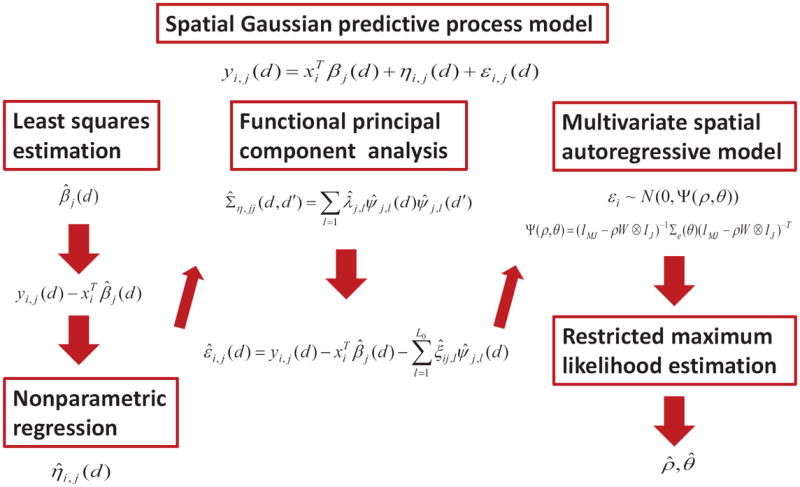
A diagram for the SGPP model with three components including a general linear model (GLM) for characterizing the association between imaging measure and covariates of interest, a functional principal component model (fPCA) to capture the global spatial dependence, and a multivariate spatial autoregressive model (SAR) to capture the local spatial dependence. The first stage of the estimation procedure is the least squares estimation of the regression coefficients β(d) = [β₁(d), …, β_J(d)], the second stage is the nonparametric estimation of Σ_η and its associated eigenvalues and eigenfunctions, and the third stage is the restricted maximum likelihood estimation of all the parameters in the spatial autoregressive model.

Stage (I) is to calculate the least squares estimate of the regression coefficients at voxel d, which are given by

$${\widehat{\beta }}_j(d)={(\sum _{i=1}^n{\mathbf{x}}_i{\mathbf{x}}_i^T)}^{-1}\sum _{i=1}^n{\mathbf{x}}_i{y}_{i,j}(d)\mathrm{for}j=1,\mathrm{\dots },J.$$ (6)

For SGPP, one may directly calculate the maximum likelihood estimate of β_j(d) by explicitly accounting for spatial correlations of imaging data. However, this is unnecessary since β̂_j(d) is exactly the maximum likelihood estimate of β_j(d) under SGPP. Specifically, SGPP can be regarded as a special case of seemingly unrelated regressions (Zellner, 1962) and the maximum likelihood estimators turn out to be numerically identical to the least squares estimators when the same set of covariates is used in all voxels. Sharing the same set of covariates across voxels is exactly the case for many neuroimaging applications. Therefore, statistically, incorporating spatial correlations of imaging data under SGPP does not lead to efficiency gain.

Instead, to gain efficiency, one needs to explicitly incorporate the spatial smoothness of imaging data (Polzehl et al., 2010; Li et al., 2011; Groves et al., 2009; Penny et al., 2005; Brezger et al., 2007; Smith and Fahrmeir, 2007). For instance, in Polzehl et al. (2010) and Li et al. (2011), various novel propagation-separation methods were developed for a large class of parametric models by explicitly assuming piecewise smoothness of imaging data. Under the Bayesian framework, various MRF spatial priors were used to primarily capture spatial smoothness, not spatial correlations, of imaging data (Groves et al., 2009; Penny et al., 2005; Brezger et al., 2007; Smith and Fahrmeir, 2007). Although we may use such estimation methods to refine β̂_j(d), we avoid such refinement for simplicity, since our primary interest focuses on predicting imaging data.

Stage (II) is to estimate Σ_η and its eigenvalues and eigenfunctions. Stage (II) consists of three steps as follows.

• Step (II.1) is to calculate all individual functions η_i,j(d) by using nonparametric regression techniques. We may apply the local linear regression method to $y_{i,j}\left(d\right)-{\mathbf{x}}_i^T{\widehat{\beta }}_j\left(d\right)$ as shown in Zhu et al. (2011). Alternatively, we may use a spatial smoothing technique based on the neighborhood structure for graph data, such as data based on the cortical and subcortical surface geometry or structural and functional connectivity matrices (Grenander and Miller, 2007). Specifically, we use the locally weighted average method (Waller and Gotway, 2004) to estimate η̂_i,j(d) by

  $${\widehat{\eta }}_{i,j}(d)=\frac{1}{2}(y_{i,j}(d)-{\mathbf{x}}_i^T{\widehat{\beta }}_j(d))+\frac{1}{2}\frac{{\mathrm{\sum }}_{m=1}^{M}1(d_m\in N(d))(y_{i,j}(d_m)-{\mathbf{x}}_i^T{\widehat{\beta }}_j(d_m))}{{\mathrm{\sum }}_{m=1}^{M}1(d_m\in N(d))},$$ (7)

  where 1(·) denotes an indicator function of an event.
• Step (II.2) is to estimate Σ_η(d, d′) by using the empirical covariance matrix of η̂_i(d) = (η̂_i,₁(d), … , η̂_i,J (d))^T as follows:

  $${\widehat{\mathrm{\sum }}}_{\eta }(d,d^{\prime })={(n-p)}^{-1}\sum _{i=1}^n{\widehat{\mathit{\eta }}}_i(d){\widehat{\mathit{\eta }}}_i{(d^{\prime })}^T.$$ (8)

  Then, we can use the spectral decomposition of (8) to estimate the eigenvalue-eigenvector pairs of Σ_η(d, d′) in (2). Since higher order principal components are much harder to estimate and interpret, only a finite number of principal components are assumed to be relevant. Typically the value L₀ in (3) is chosen based on the proportion of explained variance (Zipunnikov et al., 2011; Greven et al., 2010a; Zhu et al., 2011; Di et al., 2009). Similar to the method in Zhu et al. (2011), we chose the number of principal components in a way that the proportion of the cumulative eigenvalue is at least 80%. These choices worked well in our simulations and application.
• Step (II.3) is to compute the functional principal component scores ξ_i,j,l. The (j, l)-th functional principal component score of the i-th subject can be approximated by

  $${\widehat{\xi }}_{ij,l}=\sum _{m=1}^M{\widehat{\eta }}_{i,j}\left(d_m\right){\widehat{\psi }}_{j,l}\left(d_m\right)V\left(d_m\right),$$ (9)

  where V(d_m) is the volume of voxel d_m.

Stage (III) is to estimate the parameters in the SAR model. First, following Schabenberger and Gotway (2004) and Carlin and Banerjee (2003), we define a proximity matrix given by W = [w_mm′]_m=1, … ,_M; _m′=1,…,M, where w_mm′ = |N(d_m|⁻¹ 1(d_m′ ∈ N (d_m)). Then (4) can be written as

$$\left({\mathbf{I}}_{MJ}-\rho \mathbf{W}\otimes {\mathbf{I}}_J\right){\epsilon }_i={\mathbf{e}}_i,$$ (10)

where I_K denotes a K × K identity matrix for any integer K, ε_i = (ε_i(d₁)^T ,…, ε_i(d_M)^T)^T, e_i = (e_i(d₁)^T ,…, e_i(d_M)^T)^T, and ⊗ denotes the Kronecker product. We can directly estimate the unknown parameters of model (10), whose details are given in Appendix A.

2.3. Prediction Procedure

We present a prediction procedure to estimate the prediction accuracy of the proposed SGPP model. We start with splitting the data set into a training set and a test set. We fit the SGPP model to the training set to estimate the regression coefficients, denoted as β̂_j;TR(d), eigenvalue-eigenfunction pairs, denoted as { (λ̂_j,l;TR, ψ̂_j,l;TR(d)) : l = 1,…, L₀}, and the REML estimates of SAR parameters (ρ_TR, θ̂_TR), denoted as (ρ̂_TR, θ̂_TR).

Then we use a prediction procedure given below to predict the multiple measurements at the hold-out voxels, based on the measurements at other voxels and the fitted model, for each subject in the test set.

Without loss of generality, we assume that D_mis is the set of all voxels with missing data for the i₀-th subject. Here, the number of voxels in D_mis can be relatively large compared with that in D. The prediction procedure consists of three steps as follows.

• Step (III.1) is to estimate ξ_i0j,ℓ, denoted by ξ̂_i0j,ℓ;TE, for l = 1, …, L₀. First, we estimate η_i0,j (d), denoted as η̂_i0,j;TE(d), for all d ∈ D \ D _mis. We will apply the nonparametric methods described in Step (II.1). Second, since ψ̂_j,l;TR(d) and η̂_i0,_j;TE (d) are known for all d ∈ D \ D_mis, it follows from (3) that estimating ξ̂_i0j,ℓ;TE is equivalent to solving a linear model given by

  $${\widehat{\eta }}_{i0,j;\mathit{TE}}\left(d\right)\approx \sum _{l=1}^{L_0}{\xi }_{i0j,l}{\widehat{\psi }}_{j,l;\mathit{TR}}\left(d\right)\mathrm{for}d\in D\backslash D_{\mathit{mis}}.$$ (11)

  If the number of voxels in D \ D_mis is larger than L₀, which is usually small, then we can calculate the least squares estimate of ξ_i0j = (ξ_i0j,₁, ⋯, ξ_i0j, L₀)^T given by

  $${\widehat{\mathbf{\xi }}}_{i0j\mathbf{;}\mathit{TE}}=\mathrm{argmin}{\xi }_{i0j}\sum _{d\in D\backslash D_{\mathit{mis}}}{\left[{\widehat{\eta }}_{i0,j;\mathit{TE}}\left(d\right)-\sum _{l=1}^{L_0}{\xi }_{i0j,l}{\widehat{\psi }}_{j,l;\mathit{TR}}\left(d\right)\right]}^2.$$ (12)

• Step (III.2) is to estimate ε_i0,_j (d), denoted by ε̂_i0j;TE(d), for all d ∈ D. First, we will calculate ${\widehat{\epsilon }}_{i_0,j;TE}\left(d\right)=y_{i_0,j}\left(d\right)-{\mathbf{x}}_{i_0}^T{\widehat{\beta }}_j\left(d\right)-{\sum }_{l=1}^{L_0}{\widehat{\xi }}_{i_{0}j,l;\mathit{TE}}{\widehat{\psi }}_{j,l;\mathit{TR}}\left(d\right)$ for all d ∈ D\D_mis. Second, we will use the kriging method to calculate ε̂_i0j;TE(d) for all d ∈ D_mis.

• Step (III.3) is to predict y_i0,_j(d) according to

  $${\widehat{y}}_{i_0,j}\left(d\right)={\mathbf{x}}_{i_0}^T{\widehat{\beta }}_{j;\mathit{TR}}\left(d\right)+\sum _{l=1}^{L_0}{\widehat{\xi }}_{i_{0}j,l\mathit{TE}}{\widehat{\psi }}_{j,l;\mathit{TR}}\left(d\right)+{\widehat{\mathrm{\epsilon }}}_{i_0,j;\mathit{TE}}\left(d\right)\mathrm{for}d\in D_{\mathit{mis}}.$$ (13)

2.4. Model Validation

For each subject in the test set, we apply the prediction procedure described in Section 2.3 to predict the partially missing imaging data. We evaluate the prediction accuracy of the proposed model by quantifying the prediction error at all voxels with missing data. Specifically the rtMSPE for each j is given by

$$\mathrm{rtMSPE}\left(j\right)=\sqrt{\frac{1}{\left|S_{\mathit{TE}}\right|\left|D_{\mathit{mis}}\right|}\sum _{i\in S_{\mathit{TE}}}\sum _{d_m\in D_{\mathit{mis}}}{({\widehat{y}}_{i,j}\left(d_m\right)-y_{i,j}\left(d_m\right))}^2},$$ (14)

where S_TE denotes the set of all subjects in the test set, |S_TE| and |D_mis| are, respectively, the cardinality of S_TE and D_mis. We also calculate the rtMSPE for several competing methods, such as the voxel-wise linear model (VWLM), and compare their prediction accuracy.

3. Simulation Studies

In this section, we use simulation examples to investigate the finite sample performance of SGPP. First, we use Gaussian random fields to simulate random samples in order to examine the accuracy of all parameter estimates in model (5) and evaluate the predictive performance of model (5) using rtMSPE. Second, we use a class of non-Gaussian random fields to simulate random samples in order to examine the robustness of SGPP.

3.1. Gaussian Random Fields

We simulated data at all 900 pixels on a 30 × 30 phantom image for n = 50 subjects. At a given pixel d_m = (d_m1, d_m2)^T , the data were generated from a bivariate spatial Gaussian process model according to

$$y_{i,j}\left(d_m\right)={\beta }_{j1}\left(d_m\right)+x_{i2}{\beta }_{j2}\left(d_m\right)+{\eta }_{i,j}\left(d_m\right)+{\epsilon }_{i,j}\left(d_m\right),i=1,\dots ,50;j=1,2,$$ (15)

where x_i2 were generated independently from the uniform distribution on [1, 2]. We set ${\eta }_{i,j}\left(d_m\right)={\sum }_{l=1}^2{\xi }_{ij,l}{\psi }_{j,l}\left(d_m\right)$, where ξ_i,j,l are independently generated according to ξ_i1,l ~ N(0, 14²), ξ_i1,2 ~ N(0, 7²), ξ_i2,1 ~ N(0, 15²), and ξ_i2,2 ~ N(0, 7²). The regression coefficients and eigenfunctions were set as follows:

$$\begin{array}{ll}{\beta }_{11}\left(d_m\right)=d_{m1}^{1/2},{\beta }_{12}\left(d_m\right)=1/\left(d_{m1}+d_{m2}\right),\hfill & {\beta }_{21}\left(d_m\right)=0.1\left(d_{m1}+d_{m2}\right),{\beta }_{22}\left(d_m\right)=1/d_{m2};\hfill \\ {\psi }_{1,1}\left(d_m\right)=-\frac{1}{15\sqrt{2}}\sin \left(\pi \left(d_{m1}+d_{m2}\right)/15\right),\hfill & {\psi }_{1,2}\left(d_m\right)=\frac{1}{15\sqrt{2}}\cos \left(\pi \left(d_{m1}+d_{m2}\right)/15\right);\hfill \\ {\psi }_{2,1}\left(d_m\right)=-\frac{1}{15\sqrt{2}}\sin \left(\pi \left(d_{m1}+d_{m2}\right)/30\right),\hfill & {\psi }_{2,2}\left(d_m\right)=\frac{1}{15\sqrt{2}}\cos \left(\pi \left(d_{m1}+d_{m2}\right)/30\right).\hfill \end{array}$$

We also generated ε_i = (ε_i(d₁)^T,…, ε_i(d₉₀₀)^T)^T from N(0, Ψ (ρ, θ)), where ρ = 0.9 and θ was chosen in a way that Σ_e (θ) = I₉₀₀ ⊗ diag(0.278, 0.04). In this case, we impose the homogeneous variance assumption across all voxels.

We fitted the model (5) to the simulated data using the estimation procedure described in Section 2.2. Figure 2 shows the true β_j (d) and β̂_j (d) for j = 1, 2. As shown in Figure 2, β̂_j (d) detects the patterns in the true regression coefficients, but the estimated regression coefficients are also affected by the large scale spatial variation, and the variance appears to be large. Following the method described in Section 2.2, we estimated η_i,j(d) based on $y_{i,j}\left(d\right)-{\mathbf{x}}_i^T{\widehat{\beta }}_j\left(d\right)$ using the locally weighted average method. For simplicity, we used the uniform weight to calculate η̂_i,j(d). We also plotted the relative eigenvalues of Σ̂_η,jj(d, d′) for j = 1, 2 in Figure 3 (a), where the relative eigenvalues are defined as the ratios of the eigenvalues over their sum. It is shown that the first two eigenvalues account for about 80% of the total variation and the others quickly vanish to zero. We present the estimated eigenfunctions corresponding to the largest two eigenvalues along with the true eigenfunctions for j = 1, 2 in Figure 4. It shows that ${\sum }_{l=1}^2{\widehat{\xi }}_{ij,l}{\widehat{\psi }}_{j,l}\left(d\right)$ can capture the main feature in the true eigenfunctions. The parameters of the spatial autoregressive model were estimated by optimizing the REML function (17). We calculated the mean of the parameter estimates based on the results from the 50 simulated data sets and obtained ρ̂ = 0.89 and Σ_e(θ̂) given by

$${\sum }_e\left(\widehat{\theta }\right)={\mathbf{I}}_{900}\otimes \left(\begin{array}{cc}0.0269& -0.0000\\ -0.0000& 0.0385\end{array}\right),$$

which are close to the true ρ = 0.9 and Σ_e(θ) = I₉₀₀ ⊗ diag(0.0278, 0.04).

Fig. 2.

Simulation results for the Gaussian random field: (a) true β₁₁(d); (b) true β₁₂(d); (c) true β₂₁(d); (d) true β₂₂(d); (e) β̂₁₁(d); (f) β̂₁₂(d); (g) β̂₂₁(d); (h) β̂₂₂(d).

Fig. 3.

The first 10 relative eigenvalues of Σ̂_η,jj (d,d′) for (a) simulation results for the Gaussian random field and (b) the surface data of the left lateral ventricle.

Fig. 4.

Simulation results for the Gaussian random field: (a) true ψ_1,1(d); (b) true ψ_1,2(d); (c) true ψ_2,1(d); (d) true ψ^2,2(d); (e) ψ̂_1,1(d); (f) ψ̂_1,2(d); (g) ψ̂_2,1(d); and (h) ψ̂_2,2(d).

Next, we examine the predictive performance of the proposed model by applying the prediction procedure in Section 2.3 to the simulated data. We splitted the data set into a test set of 15 randomly selected subjects and a training set of the other 35 subjects. For each subject in the test set, we considered the imaging data with 10%, 30%, and 50% missingness, respectively. The pixels in D_mis were randomly sampled according to the missingness. We first fitted the SGPP model to the training set and estimated the regression coefficients, eigenvalue-eigenvector pairs, and the autoregressive model parameters. Then we predicted the missing data in the test set and obtained the rtMSPE. We compare the rtMSPE for the proposed model with those for VWLM, GLM+fPCA model, and GLM+SAR model in Table 1. The SGPP model clearly outperforms the other methods. It is also shown that accounting for the global and local spatial dependences substantially increases the prediction accuracy.

Table 1.

rtMSPE for the simulated data with a Gaussian error process

Missingness		VWLM	GLM+fPCA	GLM+SAR	SGPP
10%	j = 1	0.5617	0.3203	0.4843	0.1707
	j = 2	0.6162	0.3611	0.5342	0.1966
30%	j = 1	0.5552	0.3189	0.4749	0.1736
	j = 2	0.6219	0.3700	0.5458	0.2094
50%	j = 1	0.5606	0.3205	0.4862	0.1837
	j = 2	0.6212	0.3707	0.5424	0.2181

3.2. Non-Gaussian Random Fields

We simulated data at all 900 pixels on a 30 × 30 phantom image for n = 50 subjects according to (15) with ε_i = (ε_i(d₁)^T, … , ε_i(d₉₀₀)^T)^T generated from a non-Gaussian random field. A class of non-Gaussian random fields is obtained by squaring the Gaussian random fields whose correlations are the square root of the desired correlations (Hyun et al., 2012). We subtracted the mean vector from the non-Gaussian random vector thereby obtained and scaled it so that the resulting ε_i can have zero mean vector and the covariance matrix Ψ (ρ, θ), where ρ = 0.9 and θ was chosen in a way that Σ_e(θ) = I₉₀₀ ⊗ diag(0.0278, 0.04). We applied the predictive methods discussed above to the simulated data and obtained the rtMSPE from the test set of 15 randomly selected subjects. The results are summarized in Table 2, which shows that the SGPP model performs quite well even when the data have a skewed distribution.

Table 2.

rtMSPE for the simulated data with a non-Gaussian error process

Missingness		VWLM	GLM+fPCA	GLM+SAR	SGPP
10%	j = 1	0.5810	0.3537	0.4854	0.1782
	j = 2	0.7085	0.4027	0.6241	0.2147
30%	j = 1	0.5722	0.3407	0.4800	0.1835
	j = 2	0.7245	0.4053	0.6439	0.2254
50%	j = 1	0.5684	0.3334	0.4856	0.1924
	j = 2	0.7177	0.3930	0.6415	0.2333

4. Real Data Analysis

We applied the SGPP model to the surface data of the left lateral ventricle. The surface data set of the left lateral ventricle consists of 43 infants (23 males and 20 females) at the age 1. The gestational ages of the 43 infants range from 234 to 295 days and their mean gestational age is 263 days with standard deviation 12.8 days. The responses were based on the SPHARM-PDM representation of lateral ventricle surfaces. We use the SPHARM-PDM (Styner et al., 2004) shape representation to establish surface correspondence and align the surface location vectors across all subjects. The sampled SPHARM-PDM is a smooth, accurate, fine-scale shape representation. The left lateral ventricle surface of each infant is represented by 1002 location vectors with each location vector consisting of the spatial x, y, and z coordinates of the corresponding vertex on the SPHARM-PDM surface.

We fitted the model (5) to the 3×1 coordinate vectors on the SPHARM-PDMs of the left lateral ventricle. Specifically, we set x_i = (1, G_i, Gagei_i)^T, where G_i and Gage_i, respectively, denote the gender (1 for female and 0 for male) and the gestational age of the i-th infant. We applied the estimation procedure described in Section 2.2. Figure 5 presents the estimated regression coefficients β̂(d) associated with the x, y, and z coordinates on the left lateral ventricle surface. The intercept surfaces (all panels in the first column of Figure 5) describe the overall trend of the three coordinates. We present the relative eigenvalues and eigenfunctions of Σ̂_η,jj(d, d′) for j = 1, 2, 3 in Figures 3 (b) and 6, respectively. We observe that the first five eigenvalues account for more than 80% of the total variation and the others quickly vanish to zero. We calculated the REML estimate ρ̂ and Σ_e(θ(d)).

Fig. 5.

Results from the surface data of the left lateral ventricle: (a) and (b) β̂₁₁(d), β̂₁₂(d), and β̂₁₃(d) (from left to right); (c) and (d) β̂₂₁(d), β̂₂₂(d), and β̂₂₃(d) (from left to right); (e) and (f) β̂₃₁(d), β̂₃₂(d), and β̂₃₃(d) (from left to right).

Fig. 6.

Results from the surface data of the left lateral ventricle: (a) and (b) ψ̂_1,1(d), ψ̂_1,2(d), and ψ̂_1,3(d) (from left to right); (c) and (d) ψ̂_2,1(d), ψ̂_2,2(d), and ψ̂_2,3(d) (from left to right); (e) and (f) ψ̂_3,1(d), ψ̂_3,2(d), and ψ̂_3,3(d) (from left to right).

We statistically tested the effects of the gender and gestational age on the x, y, and z coordinates of the left lateral ventricle surface. Specifically, we calculated the Wald test statistics and their corresponding p-values to test H₀ : β_j2(d) = 0 against H₁ : β_j2(d) ≠ 0 for the gender effect and H₀ : β_j3(d) = 0 against H₁ : β_j3(d) ≠ 0 for the gestational age effect across all voxels for j = 1, 2, 3. The −log₁₀(p) values are shown in Figure 7(a)-(f). We applied the false discovery rate (FDR) procedure (Benjamini and Hochberg, 1995) to correct the p-values for multiple comparisons, and the −log₁₀(p) images for the resulting adjusted p-values are shown in Figure 7 (g)-(l). The values that are greater than 1.3 indicate a significant effect at 5% significance level; they indicate a highly significant effect at 1% significance level if they are greater than 2.

Fig. 7.

Results from the surface data of the left lateral ventricle: –log₁₀(p) maps for testing H₀ : β₁₂(d) = 0 for raw p-value in (a) and for corrected p-value in (g); those for testing H₀ : β₁₃(d) = 0 for raw p-value in (b) and for corrected p-value in (h); those for testing H₀ : β₂₂(d) = 0 for raw p-value in (c) and for corrected p-value in (i); those for testing H₀ : β₂₃(d) = 0 for raw p-value in (d) and for corrected p-value in (j); those for testing H₀ : β₃₂(d) = 0 for raw p-value in (e) and for corrected p-value in (k); those for testing H₀ : β₃₃(d) = 0 for raw p-value in (f) and for corrected p-value in (l).

No gender differences were found for all coordinates of the SPHARMPDM representation of lateral ventricle surfaces. There are significant overall age effects on y and z coordinates (Figure 7 (j) and (l)). It indicates that increased volumes occurring in the lateral ventricles during the first year of life are due to widespread morphometric changes across the entire shape (Figure 7). Anterior and posterior sections of the lateral ventricle experience a large degree of outward change while the middle sections of the ventricle experience little change. Differences are primarily localized in the frontal and occipital horns of the lateral ventricle (Figure 7).

We randomly selected 13 infants and estimated the prediction error of the SGPP model by (14). The voxels with missing data were randomly sampled according to 10%, 30%, and 50% missingness, respectively. We first fitted the model (5) to the training set of the other 30 infants to estimate the regression coefficients β_j(d), eigenvalue-eigenvector pairs, and the autoregressive model parameters. We used the fitted model to predict the missing coordinate vectors in the test set and calculated the rtMSPE for each component of the vector. The results are summarized in Table 3 along with the rtMSPE for the VWLM and GLM+fPCA model, respectively. We find that the gains in the prediction accuracy are dramatic when switching from VWLM to the SGPP model. For the case of 10% missingness, the rtMSPE was reduced by 95 to 96% using the SGPP model as compared with VWLM for all three components of the vector; it was also reduced by 92% as compared with GLM+fPCA model. For the case of 50% missingness, the decreases were still 90 to 92% as compared with VWLM and 84% as compared with GLM+fPCA model for all three components of the vector.

Table 3.

rtMSPE for the surface data of the left lateral ventricle

Missingness		VWLM	GLM+fPCA	SGPP
10%	x-coordinate	1.9272	0.9810	0.0738
	y-coordinate	2.2448	1.3455	0.1067
	z-coordinate	2.1554	1.1753	0.0926
30%	x-coordinate	1.9337	1.0197	0.1156
	y-coordinate	2.2655	1.3827	0.1657
	z-coordinate	2.1906	1.2069	0.1446
50%	x-coordinate	1.9263	1.0294	0.1615
	y-coordinate	2.2012	1.3471	0.2204
	z-coordinate	2.1862	1.1830	0.1924

Table 3 shows that the SGPP model substantially increases the prediction accuracy compared with the other two models. They also suggest that the fPCA model can effectively capture the medium-to-long-range spatial dependence, but the fPCA model alone may not be effective in accounting for local spatial dependence. In contrast, the SGPP model can effectively account for the long-to-medium-to-short-range dependence leading to more accurate prediction.

5. Discussion

We have proposed a spatial Gaussian predictive process (SGPP) framework for the spatial analysis of imaging measures. The fPCA+SAR components in SGPP allow us to accurately approximate the unstructured variancecovariance matrix of ultra-high dimensional data by explicitly modeling the long-to-medium-to-short-range spatial dependence. Thus, due to the computational efficiency of fPCA+SAR, SGPP is a powerful predictive model for efficiently handling high-dimensional imaging data compared with other methods in the literature (Bowman et al., 2008; Bowman, 2007; Derado et al., 2012; Groves et al., 2009; Penny et al., 2005; Brezger et al., 2007; Smith and Fahrmeir, 2007; Guo et al., 2008). We have developed a three-stage estimation procedure and presented a predictive method under the SGPP model. Through simulation studies and a real data example, we have shown that the SGPP model substantially outperforms VWLM, GLM+fPCA, and GLM+SAR in terms of prediction accuracy.

While our prediction results in Table 3 can be used as a validation of SGPP in real applications, SGPP and our prediction method can be used to directly solve missing data problems in neuorimaging studies. For instance, missing data in some brain regions may occur due to data acquisition limits and susceptibility artifact (see e.g. Higdon et al., 2004; Vaden et al., 2012). The existing approaches for handling such missing imaging data are primarily based on imputation methods, which do not account for the local and global spatial correlation structures of imaging data (Higdon et al., 2004; Uijl et al., 2008). For example, in (Uijl et al., 2008), a single imputation method based on linear regression has been used to replace missing positron emission tomography data in order to predict epilepsy surgery outcome. Recently, in (Vaden et al., 2012), a regression based multiple imputation approach also leverages the local spatial information in fMRI data by using imaging data in neighboring voxels as covariates in the regression model. However, these multiple imputation procedures are not practical under the presence of the large amounts of imaging data besides its heavy numerical burden (Higdon et al., 2004). In contrast, as shown in the simulations and real data example, SGPP can predict the missing data very accurately even for large proportion of missingness as large as 50%.

Our SGPP can be regarded as a natural extension of spatial mixed effects models developed for the analysis of geostatistical data Sang and Huang (2012). The predictive process in the spatial mixed effects models also uses some fixed basis functions to capture major variation in geostatistical data Banerjee et al. (2008). However, for geostatistical data, basis functions are pre-specified and the Nyström method in (Sang and Huang, 2012; Cressie and Johannesson, 2008b; Stein, 2008), whereas SGPP uses fPCA to directly estimate spatial basis functions and allow varying regression coefficients across the brain, since most neuroimaging studies usually contain multiple subjects.

Several important issues need to be addressed in future research. The basic setup of the proposed model can be extended to neuroimaging data obtained from clustered studies (e.g., longitudinal, twin, or familial). Longitudinal neuroimaging studies are primarily carried out in order to characterize individual change in neuroimaging measurements (e.g., volumetric and morphometric measurements) over time, and the effect of some covariates (or predictors) of interest, such as diagnostic status and gender, on the individual change (Evans and Group., 2006). A key feature of longitudinal neuroimaging data is that it usually has a strong temporal correlation, that is, imaging measurements of the same individual usually exhibit positive correlation and the strength of the correlation decreases with the time separation. In this case, we will extend (1) by including a longitudinal fPCA model in (Greven et al., 2010b; Yuan et al., 2013) to incorporate the long-to-medium range of spatial-temporal correlation and a longitudinal SAR model to incorporate the medium-to-short range of spatial-temporal correlation. In this case, one may gain statistical power of testing hypothesis of interest by explicitly modeling spatial-temporal correlation (Derado et al., 2010).

The key idea of SGPP can also be extended to predict ‘missing’ neuroimaging data in different scenarios. For instance, SGPP can be extended to predict follow-up structural alternation and neural activity based on an individual’s baseline image (Derado et al., 2012; Bowman et al., 2008). Moreover, SGPP may be useful for predicting clinical outcomes, such as disease diagnosis and prevention (Ryali et al., 2010; Hinrichs et al., 2009; Martino et al., 2008). Although a large family of methods has been developed for supervised learning (Hastie et al., 2009), most supervised learning methods coupled with dimension reduction methods do not account for the long-tomedium-to-short range spatial structure of imaging data. As shown above, since SGPP provides an excellent ‘low-dimensional’ representation of highdimensional imaging data, we may use such low-dimensional representation based on SGPP as a feature vector to build a prediction model (e.g., linear regression, logistic regression, or support vector machine) to predict clinical outcomes.

Highlights.

• Develop a SGPP for predictive analysis of neuroimaging data.

• Useful for characterizing spatial correlation of neuroimaging data.

• Achieving high prediction accuracy for simulated and real imaging data.

Appendix A. Estimation Procedure for (ρ, θ)

Since e_i ~ N (0, Σ_e(θ)), it follows from(10) that ε_i is a multivariate normal random vector with zero mean and covariance matrix given by

$$\mathbf{\Psi }(\rho ,\mathit{\theta })={({\mathbf{I}}_{MJ}-\rho \mathbf{W}\otimes {\mathbf{I}}_J)}^{-1}{\mathrm{\sum }}_e(\mathit{\theta }){({\mathbf{I}}_{MJ}-\rho \mathbf{W}\otimes {\mathbf{I}}_J)}^{-T},$$ (16)

where Σ_e(θ) is a block diagonal matrix with elements Σ_e(θ(d)) across d ∈ D. We assume that Σ_e(θ(d)) = [L(θ(d))L(θ(d))^T]⁻¹, where L (θ(d)) is a J × J lower triangular matrix with strictly positive diagonal entries of the Cholesky factorization of Σ_e(θ(d))⁻¹.

To estimate (ρ, θ), we proceed as follows. First, according to (5), (6), and (9), we can estimate ε_i,j(d) by using ${\widehat{\epsilon }}_{i,j}\left(d\right)=y_{i,j}\left(d\right)-{\mathbf{x}}_i^T{\widehat{\beta }}_j\left(d\right)-{\sum }_{l=1}^{L_0}{\widehat{\xi }}_{ij,l}{\widehat{\psi }}_{j,l}\left(d\right)$. We define ε̂_i = (ε̂_i(d₁)^T,…, ε̂_i(d_M)^T)^T and $\widehat{\mathit{\epsilon }}={\left({\widehat{\mathit{\epsilon }}}_1^T,\dots ,{\widehat{\mathit{\epsilon }}}_n^T\right)}^T$. Second, we calculate a restricted maximum likelihood estimate (REML) of (ρ, θ) by maximizing a log-restricted maximum likelihood function given by

$$\begin{array}{c}L(\rho ,\mathit{\theta }|\widehat{\mathit{\epsilon }})=\mathrm{constant}+\frac{n}{2}\log |\mathbf{\Psi }{(\rho ,\mathit{\theta })}^{-1}|-\frac{1}{2}\log |{\mathbf{Z}}^T\mathbf{\Psi }{(\rho ,\mathit{\theta })}^{-1}\mathbf{Z}|\\ -\frac{1}{2}\sum _{i=1}^n{({\widehat{\mathit{\epsilon }}}_i-\mathbf{Z}\widehat{\mathit{\mu }}(\rho ,\mathit{\theta }))}^T\mathbf{\Psi }{(\rho ,\mathit{\theta })}^{-1}({\widehat{\mathit{\epsilon }}}_i-\mathbf{Z}\widehat{\mathit{\mu }}(\rho ,\mathit{\theta })),\end{array}$$ (17)

where $\widehat{\mathit{\mu }}(\mathit{\rho },\theta )={(n{\mathbf{Z}}^T\mathbf{\Psi }{(\rho ,\mathit{\theta })}^{-1}\mathbf{Z})}^{-1}{\sum }_{i=1}^n{\mathbf{Z}}^T\mathit{\Psi }{(\rho ,\mathbf{\theta })}^{-1}{\widehat{\mathit{\epsilon }}}_i$ and Z is an M J × J matrix of (I_J, … , I_J)^T. Furthermore, Ψ(ρ, θ)⁻¹ is given by

$$\mathbf{\Psi }{(\rho ,\mathit{\theta })}^{-1}={({\mathbf{I}}_{MJ}-\rho \mathbf{W}\otimes {\mathbf{I}}_J)}^T\mathrm{diag}((L(\mathit{\theta }(d))L{(\mathit{\theta }(d))}^T)({\mathbf{I}}_{MJ}-\rho \mathbf{W}\otimes {\mathbf{I}}_J).$$

Although Ψ(ρ, θ) is an extremely large matrix, Ψ(ρ, θ)⁻¹ is a very sparse matrix, which makes the numerical optimization of L(ρ, θ|ε̂) feasible.

To optimize (17) with respect to ρ and θ, we used a grid search method for the parameter ρ ranging between 0.1 and 0.99 with finer grids in the upper range of ρ. For a fixed value of ρ, we optimized the REML function using the Matlab function fmincon, which implements a Quasi-Newton method (Broyden-Fletcher-Goldfarb-Shanno method). The computation was done in matlab on Intel Corei7-2700K, CPU 3.50 GHz and 32 GB RAM. For one replicate of bivariate data at 900 pixels with 50 subjects it took about 70 minutes to optimize the REML function. The computational time for the SGPP model might be reduced by using other programming languages, such as C++.

Appendix B. Spatial Prediction using Kriging

We describe the spatial prediction using kriging at Step (III.2) in detail. Since predictions are made for multiple measurements at each voxel, we apply a co-kriging technique to obtain ε̂_{i0;T E}(d) for d ∈ D_mis. The co-kriging predictor is a best linear unbiased predictor (BLUP) given by

$${\widehat{\mathit{\epsilon }}}_{i_0;\mathit{TE}}(d)=\sum _{d_m\in D\backslash D_{\mathit{mis}}}{\mathbf{\Gamma }}_m{\widehat{\mathit{\epsilon }}}_{i_0}(d_m),$$ (18)

where each Г_m is a J × J matrix and (…, Г_m, …) is given by

$$\left(\dots ,{\mathrm{\sum }}_{\epsilon }\left(d,d_m\right),\dots \right){\left({\mathrm{\sum }}_{\epsilon }\left(d_m,d_{m^{\prime }}\right)\right)}^{-1},$$ (19)

where (Σ_ε (d_m, d_m′)) denotes the covariance matrix of (…,ε_i0(d_m)^T, …)^T for d_m ∈ D\D_mis. Then the matrices in the RHS of (19) are obtained from (16) with the REML estimates, (^ρ_TR, θ̂_TR) plugged in.

References

- Ball T, Breckel TP, Mutschler I, Aertsen A, Schulze-Bonhage A, Hennig J, Speck O. Variability of fmri-response patterns at different spatial observation scales. Human Brain Mapping. 2012;33:1155–1171. doi: 10.1002/hbm.21274. [DOI] [PMC free article] [PubMed] [Google Scholar]
- Banerjee S, Gelfand AE, Finley AO, Sang H. Gaussian predictive process models for large spatial data sets. Journal of the Royal Statistical Society: Series B (Statistical Methodology) 2008;70:825–848. doi: 10.1111/j.1467-9868.2008.00663.x. [DOI] [PMC free article] [PubMed] [Google Scholar]
- Benjamini Y, Hochberg Y. Controlling the false discovery rate: a practical and powerful approach to multiple testing. Journal of the Royal Statistical Society Series B (Methodological) 1995:289–300. [Google Scholar]
- Bowman FD. Spatio-temporal models for region of interest analyses of functional mappping experiments. Journal of American Statistical Association. 2007;102:442–453. [Google Scholar]
- Bowman FD, Caffo BA, Bassett S, Kilts C. Bayesian hierarchical framework for spatial modeling of fmri data. NeuroImage. 2008;39:146–156. doi: 10.1016/j.neuroimage.2007.08.012. [DOI] [PMC free article] [PubMed] [Google Scholar]
- Brezger A, Fahrmeir L, Hennerfeind A. Adaptive gaussian markov random fields with applications in human brain mapping. Journal of the Royal Statistical Society: Series C. 2007;56:327–345. [Google Scholar]
- Carlin BP, Banerjee S. Bayesian Statistics 7. Oxford University Press; Oxford: 2003. Hierarchical multivariate car models for spatio-temporally correlated survival data; pp. 45–63. [Google Scholar]
- Chiou JM, Muller HG, Wang JL, et al. Functional response models. Statistica Sinica. 2004;14:675–694. [Google Scholar]
- Cressie N, Johannesson G. Fixed rank kriging for very large spatial data sets. J Roy Statist Soc B. 2008a;70:825–848. doi: 10.1111/j.1467-9868.2008.00663.x. [DOI] [PMC free article] [PubMed] [Google Scholar]
- Cressie N, Johannesson G. Fixed rank kriging for very large spatial data sets. Journal of the Royal Statistical Society: Series B (Statistical Methodology) 2008b;70:209–226. doi: 10.1111/j.1467-9868.2008.00663.x. [DOI] [PMC free article] [PubMed] [Google Scholar]
- Cressie N, Wikle C. Statistics for Spatio-Temporal Data. Wiley; Hoboken, NJ: 2011. [Google Scholar]
- Cressie NA. Statistics for Spatial Data. Wiley; New York: 1993. revised edition. [Google Scholar]
- Derado G, Bowman F, Zhang L. Predicting brain activity using a bayesian spatial model. Stat Methods Med Res. 2012 doi: 10.1177/0962280212448972. in press. [DOI] [PMC free article] [PubMed] [Google Scholar]
- Derado G, Bowman FD, Kilts CD. Modeling the spatial and temporal dependence in fmri data. Biometrics. 2010;66:949–957. doi: 10.1111/j.1541-0420.2009.01355.x. [DOI] [PMC free article] [PubMed] [Google Scholar]
- Di CZ, Crainiceanu CM, Caffo BS, Punjabi NM. Multilevel functional principal component analysis. Annals of Applied Statistics. 2009;3:458–488. doi: 10.1214/08-AOAS206SUPP. [DOI] [PMC free article] [PubMed] [Google Scholar]
- Evans AC Group., BDC. The nih mri study of normal brain development. NeuroImage. 2006;30:184–202. doi: 10.1016/j.neuroimage.2005.09.068. [DOI] [PubMed] [Google Scholar]
- Gelfand AE, Vounatsou P. Proper multivariate conditional autoregressive models for spatial data analysis. Biostatistics. 2003;4:11–15. doi: 10.1093/biostatistics/4.1.11. [DOI] [PubMed] [Google Scholar]
- Grenander U, Miller MI. Pattern Theory From Representation to Inference. Oxford University Press; 2007. [Google Scholar]
- Greven S, Crainiceanu C, Caffo B, Reich D. Longitudinal functional principal component analysis. Electronic journal of statistics. 2010a;4:1022. doi: 10.1214/10-EJS575. [DOI] [PMC free article] [PubMed] [Google Scholar]
- Greven S, Crainiceanu C, Caffo B, Reich D. Longitudinal functional principal component analysis. Electron J Statist. 2010b;4:1022–1054. doi: 10.1214/10-EJS575. [DOI] [PMC free article] [PubMed] [Google Scholar]
- Groves AR, Chappell MA, Woolrich MW. Combined spatial and non-spatial prior for inference on mri time-series. NeuroImage. 2009;45:795–809. doi: 10.1016/j.neuroimage.2008.12.027. [DOI] [PubMed] [Google Scholar]
- Guo Y, Bowman DF, Kilts C. Predicting the brain response to treatment using a bayesian hierarchical model with application to a study of schizophrenia. Hum Brain Mapp. 2008;29:1092–1109. doi: 10.1002/hbm.20450. [DOI] [PMC free article] [PubMed] [Google Scholar]
- Hall P, Müller HG, Wang JL. Properties of principal component methods for functional and longitudinal data analysis. The Annals of Statistics. 2006;34:1493–1517. [Google Scholar]
- Hastie T, Tibshirani R, Friedman J. The Elements of Statistical Learning: Data Mining, Inference, and Prediction. 2. Springer; Hoboken, New Jersey: 2009. [Google Scholar]
- Higdon R, Foster NL, Koeppe RA, DeCarli CS, Jagust WJ, Clark CM, Barbas NR, Arnold SE, Turner RS, Heidebrink JL, et al. A comparison of classification methods for differentiating frontotemporal dementia from alzheimer’s disease using fdg-pet imaging. Statistics in medicine. 2004;23:315–326. doi: 10.1002/sim.1719. [DOI] [PubMed] [Google Scholar]
- Hinrichs C, Singh V, Mukherjee L, Xu G, Chung MK, Johnson SC ADNI. Spatially augmented lpboosting for ad classification with evaluations on the adni dataset. NeuroImage. 2009;48:138–149. doi: 10.1016/j.neuroimage.2009.05.056. [DOI] [PMC free article] [PubMed] [Google Scholar]
- Hyun JW, Burman P, Paul D. A regression approach for estimating the parameters of the covariance function of a stationary spatial random process. Journal of Statistical Planning and Inference. 2012;142:2330–2344. [Google Scholar]
- Jones DK, Symms MR, Cercignani M, Howard RJ. The effect of filter size on vbm analyses of dt-mri data. NeuroImage. 2005;26:546–554. doi: 10.1016/j.neuroimage.2005.02.013. [DOI] [PubMed] [Google Scholar]
- Kelejian HH, Prucha IR. Estimation of simultaneous systems of spatially interrelated cross sectional equations. Journal of Econometrics. 2004;118:27–50. [Google Scholar]
- Kissling WD, Carl G. Spatial autocorrelation and the selection of simultaneous autoregressive models. Global Ecology and Biogeography. 2008;17:59–71. [Google Scholar]
- Li Y, Gilmore J, Wang J, Styner M, Lin WL, Zhu HT. Twostage multiscale adaptive regression methods of twin neuroimaging data. IEEE Transactions on Medical Imaging. 2012;31:1100–1112. doi: 10.1109/TMI.2012.2185830. [DOI] [PMC free article] [PubMed] [Google Scholar]
- Li Y, Gilmore JH, Shen D, Styner M, Lin W, Zhu HT. Multiscale adaptive generalized estimating equations for longitudinal neuroimaging data. NeuroImage. 2013;72:91–105. doi: 10.1016/j.neuroimage.2013.01.034. [DOI] [PMC free article] [PubMed] [Google Scholar]
- Li Y, Zhu H, Shen D, Lin W, Gilmore JH, Ibrahim JG. Multiscale adaptive regression models for neuroimaging data. Journal of the Royal Statistical Society: Series B. 2011;73:559–578. doi: 10.1111/j.1467-9868.2010.00767.x. [DOI] [PMC free article] [PubMed] [Google Scholar]
- Marquand A, Howard M, Brammer M, Chu C, Coen S, Mourão-Miranda J. Quantitative prediction of subjective pain intensity from whole-brain fmri data using gaussian processes. Neuroimage. 2010;49:2178–2189. doi: 10.1016/j.neuroimage.2009.10.072. [DOI] [PubMed] [Google Scholar]
- Martino FD, Valente G, Staeren N, Ashburner J, Goebel R, Formisano E. Combining multivariate voxel selection and support vector machines for mapping and classification of fMRI spatial patterns. NeuroImage. 2008;43:44–58. doi: 10.1016/j.neuroimage.2008.06.037. [DOI] [PubMed] [Google Scholar]
- Myers DE. Matrix formulation of co-kriging. Journal of the International Association for Mathematical Geology. 1982;14:249–257. [Google Scholar]
- Penny WD, Trujillo-Barreto NJ, Friston KJ. Bayesian fMRI time series analysis with spatial priors. NeuroImage. 2005;24:350–362. doi: 10.1016/j.neuroimage.2004.08.034. [DOI] [PubMed] [Google Scholar]
- Pinheiro JC, Bates DM. Unconstrained parametrizations for variance-covariance matrices. Statistics and Computing. 1996;6:289–296. [Google Scholar]
- Polzehl J, Spokoiny VG. Propagation-separation approach for local likelihood estimation. Probab Theory Relat Fields. 2006;135:335–362. [Google Scholar]
- Polzehl J, Voss HU, Tabelow K. Structural adaptive segmentation for statistical parametric mapping. NeuroImage. 2010;52:515–523. doi: 10.1016/j.neuroimage.2010.04.241. [DOI] [PubMed] [Google Scholar]
- Qiu P. Jump surface estimation, edge detection, and image restoration. Journal of American Statistical Association. 2007;102 [Google Scholar]
- Ryali S, Supekar K, Abrams DA, Menon V. Sparse logistic regression for whole-brain classification of fmri data. NeuroImage. 2010;51:752–764. doi: 10.1016/j.neuroimage.2010.02.040. [DOI] [PMC free article] [PubMed] [Google Scholar]
- Sang H, Huang JZ. A full scale approximation of covariance functions for large spatial data sets. J Roy Statist Soc B. 2012;74:111–132. [Google Scholar]
- Schabenberger O, Gotway CA. Statistical methods for spatial data analysis. Chapman and Hall/CRC; 2004. [Google Scholar]
- Smith MS, Fahrmeir L. Spatial bayesian variable selection with application to functional magnetic resonance imaging. Journal of the American Statistical Association. 2007;102:417–431. [Google Scholar]
- Stein ML. A modeling approach for large spatial datasets. Journal of the Korean Statistical Society. 2008;37:3–10. [Google Scholar]
- Styner M, Lieberman JA, Pantazis D, Gerig G. Boundary and medial shape analysis of the hippocampus in schizophrenia. Medical Image Analysis. 2004;8:197–203. doi: 10.1016/j.media.2004.06.004. [DOI] [PubMed] [Google Scholar]
- Tabelow K, Polzehl J, Spokoiny V, Voss HU. Diffusion tensor imaging: structural adaptive smoothing. NeuroImage. 2008;39:1763–1773. doi: 10.1016/j.neuroimage.2007.10.024. [DOI] [PubMed] [Google Scholar]
- Uijl SG, Leijten FS, Arends JB, Parra J, Van Huffelen AC, Moons KG. Prognosis after temporal lobe epilepsy surgery: the value of combining predictors. Epilepsia. 2008;49:1317–1323. doi: 10.1111/j.1528-1167.2008.01695.x. [DOI] [PubMed] [Google Scholar]
- Vaden JK, Gebregziabher M, Kuchinsky SE, Eckert MA. Multiple imputation of missing fmri data in whole brain analysis original research article. NeuroImage. 2012;60:1843–1855. doi: 10.1016/j.neuroimage.2012.01.123. [DOI] [PMC free article] [PubMed] [Google Scholar]
- Wall MM. A close look at the spatial structure implied by the car and sar models. Journal of Statistical Planning and Inference. 2004;121:311–324. [Google Scholar]
- Waller LA, Gotway CA. Applied spatial statistics for public health data. Wiley-Interscience; 2004. [Google Scholar]
- Worsley KJ, Taylor JE, Tomaiuolo F, Lerch J. Unified univariate and multivariate random field theory. NeuroImage. 2004;23:189–195. doi: 10.1016/j.neuroimage.2004.07.026. [DOI] [PubMed] [Google Scholar]
- Yao F, Lee T. Penalized spline models for functional principal component analysis. Journal of the Royal Statistical Society: Series B (Statistical Methodology) 2006;68:3–25. [Google Scholar]
- Yuan Y, Gilmore JH, Geng X, Styner M, Chen K, Wang JL, Zhu H. A longitudinal functional analysis framework for analysis of white matter tract statistics. In: Wells WM, Joshi S, Pohl KM, editors. LNCS7917, Information Processing in Medical Imaging. Springer; Berlin/Heidelberg: 2013. pp. 220–231. [DOI] [PMC free article] [PubMed] [Google Scholar]
- Zellner A. An efficient method of estimating seemingly unrelated regression equations and tests for aggregation bias. Journal of the American Statistical Association. 1962;57:348–368. [Google Scholar]
- Zhao L, Boucher M, Rosa-Neto P, Evans A. Human Brain Mapping. Impact of scale space search on age- and gender-related changes in mri-based cortical morphometry. 2012 doi: 10.1002/hbm.22050. in press. [DOI] [PMC free article] [PubMed] [Google Scholar]
- Zhu H, Kong L, Li R, Styner M, Gerig G, Lin W, Gilmore JH. Fadtts: Functional analysis of diffusion tensor tract statistics. NeuroImage. 2011;56:1412–1425. doi: 10.1016/j.neuroimage.2011.01.075. [DOI] [PMC free article] [PubMed] [Google Scholar]
- Zhu HT, Gu M, Peterson BS. Maximum likelihood from spatial random effects models via the stochastic approximation expectation maximization algorithm. Statistics and Computing. 2007;15:163–177. [Google Scholar]
- Zipunnikov V, Caffo B, Yousem D, Davatzikos C, Schwartz B, Crainiceanu C. Functional principal components model for highdimensional brain imaging. Vol. 223 Johns Hopkins University, Dept of Biostatistics Working Papers; 2011. [Google Scholar]