Efficiencies for the statistics of size discrimination

Abstract

Different laboratories have achieved a consensus regarding how well human observers can estimate the average orientation in a set of N objects. Such estimates are not only limited by visual noise, which perturbs the visual signal of each object’s orientation, they are also inefficient: Observers effectively use only $\sqrt{N}$ objects in their estimates (e.g., S. C. Dakin, 2001; J. A. Solomon, 2010). More controversial is the efficiency with which observers can estimate the average size in an array of circles (e.g., D. Ariely, 2001, 2008; S. C. Chong, S. J. Joo, T.-A. Emmanouil, & A. Treisman, 2008; K. Myczek & D. J. Simons, 2008). Of course, there are some important differences between orientation and size; nonetheless, it seemed sensible to compare the two types of estimate against the same ideal observer. Indeed, quantitative evaluation of statistical efficiency requires this sort of comparison (R. A. Fisher, 1925). Our first step was to measure the noise that limits size estimates when only two circles are compared. Our results (Weber fractions between 0.07 and 0.14 were necessary for 84% correct 2AFC performance) are consistent with the visual system adding the same amount of Gaussian noise to all logarithmically transduced circle diameters. We exaggerated this visual noise by randomly varying the diameters in (uncrowded) arrays of 1, 2, 4, and 8 circles and measured its effect on discrimination between mean sizes. Efficiencies inferred from all four observers significantly exceed 25% and, in two cases, approach 100%. More consistent are our measurements of just-noticeable differences in size variance. These latter results suggest between 62 and 75% efficiency for variance discriminations. Although our observers were no more efficient comparing size variances than they were at comparing mean sizes, they were significantly more precise. In other words, our results contain evidence for a non-negligible source of late noise that limits mean discriminations but not variance discriminations.

Introduction

Our perceptions result from the combination of prior knowledge with data we gather from the environment. Of course, the visual system cannot afford to be too meticulous a scientist and measure everything. Real environments are just too complex and dynamic. Instead, the visual system often settles for being a clever statistician and quickly estimates various visual features.

Spatial orientation (i.e., tilt) is one of those visual features that can be estimated in just a glimpse, but questions remain regarding how well it can be estimated. For one thing, it is not clear why observers effectively ignore a large proportion of visible objects when estimating average tilt (e.g., Dakin, 2001). Another unanswered question is why observers effectively ignore fewer objects when estimating tilt variance. Solomon (2010) suggested one possible answer when he noted that heuristics based on the range of visible orientations afforded greater efficiency for variance estimates than they did for mean estimates.

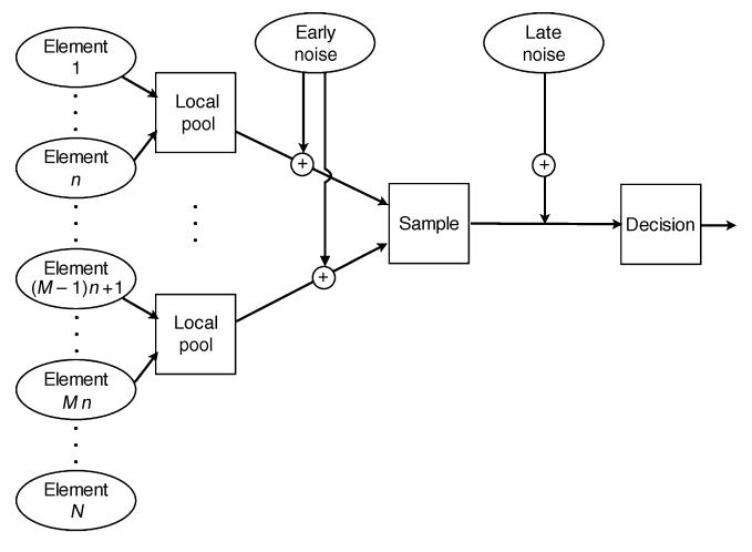
One problem with Solomon’s (2010) explanation is that it is incomplete. The relative inefficiency of mean estimates is only part of the story. His data also show that the equivalent noise for judgments of mean orientation exceeds the equivalent noise for judgments of orientation variance. (Equivalent noise is a component of the inefficient, noisy observer model sketched in Figure 1.) One peculiarity of orientation is that its mean, unlike its variance, is defined on a cyclical dimension, along which the available processing resources (e.g., Heeley, Buchanan-Smith, Cromwell, & Wright, 1997) and prior expectations (Tomassini, Morgan, & Solomon, 2010) are known to vary. Solomon wondered whether the relative imprecision of mean estimates would be observed along other dimensions that did not share this peculiarity with orientation. The current study was designed to answer that question.

Figure 1. The inefficient, noisy estimator of texture statistics.

Intuition suggests that the visual noise added to neighboring, crowded elements is more likely to be correlated than that added to distant elements. This possibility is approximated here by pooling stimulus values (e.g., orientation or size) from n neighboring elements in an effectively noise-free way. An independent, identically distributed sample of “early” Gaussian noise is then added to each pool. M pools contribute to the observer’s decision statistic, which is also subject to perturbation by Gaussian noise (i.e., “late noise”). When, as in both the current study and Solomon (2010), texture elements are demonstrably uncrowded, we can assume n = 1, and efficiency can be defined as M/N. In this case, the “local pools” effectively compute local averages, but it is conceivable that they could compute some other statistic when n ≥ 2. Both the sample size M and the late noise may vary with the observer’s task, but—by definition—early noise may vary only with the stimulus. When combined, the two sources of noise comprise the total “equivalent noise” for the observer’s task, so called because its effects can be mimicked by perturbing the stimulus itself (Pelli, 1990).

Of all the possible dimensions to examine, we selected size. The main reason for this is the controversy regarding the efficiency with which observers can estimate average size (e.g., Ariely, 2001, 2008; Chong, Joo, Emmanouil, & Treisman, 2008; Myczek & Simons, 2008). However, there is another reason, which is that we have previously found evidence for a limit to human observers’ capacity for multiple size estimates (Morgan, Giora, & Solomon, 2008). Observers in that study were asked to classify the size of one particular item in an array of distractors. The dynamic nature of the display was designed to foil any textural mechanisms that might operate on multiple sizes at once. By contrast, the paradigm used in this study requires observers to classify summary statistics of size. It therefore encourages observers to use any textural mechanisms that might be available.

Outline of the paper

Adopting the same numbering scheme used in Solomon’s (2010) paper on orientation statistics, in Experiment 1, we establish a display geometry in which there is no crowding. In Experiment 2, we measure accuracy for discriminating between arrays of circles having different mean sizes. Finally, in Experiment 3, observers were asked to discriminate between 8-circle arrays having different size variances.

Psychometric data from all these experiments are compared with the performance of an inefficient, noisy observer (e.g., Solomon, 2010). As outlined in Figure 1, both early noise and late noise are assumed to be Gaussian. Analytic computation of this model’s predictions is predicated on the assumption that each sample also stems from a Gaussian distribution. When adding external noise, we therefore wish its distribution also to be Gaussian. However, a Gaussian distribution of circle diameters does not ensure a Gaussian distribution of effective sizes for size discrimination. Although it seems reasonable to assume that there is some smooth, monotonic transformation from physical circle diameter to discriminable size, there is no guarantee that transformation is sufficiently linear to preserve the shape of the physical diameter distribution. Indeed, Weber’s law implies a logarithmic transformation (Fechner, 1860/1966). If size discriminations do, in fact, obey Weber’s law, then a lognormal distribution of circle diameters will produce a Gaussian distribution of discriminable sizes after logarithmic transduction. Our Experiment 0 was designed to verify that size discriminations do, in fact, obey Weber’s law.

Experiment 0

Weber (1851) found that “it makes no difference” whether two lines were approximately 1 or 2 inches long; the ease with which the larger could be selected depended only on the ratio of their lengths. To evaluate the possibility of an analogous law for circle sizes, we measured accuracies for discriminating otherwise identical test circles from references having diameters subtending 1.5 and 3.0 degrees of visual angle.

Methods

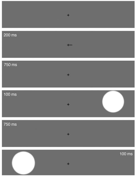
The experiment was conducted on a 15″ MacBook Pro computer, running the PsychToolbox (Brainard, 1997; Pelli, 1997; software available upon request). Display resolution was 1440 × 900 pixels. The viewing distance was 0.5 m. A typical trial is shown in Figure 2. On each trial, the two filled circles were presented asynchronously, for 0.1 s each.¹ There was a central cue cross. Either its left or right spar got longer (for 0.2 s) to indicate which side would show the first stimulus. Then, a circle was presented on that side followed (after a 0.75-s delay) by a circle on the other side. Subjects (authors JAS and CC) indicated which was larger by pressing “0” if the right side disk was larger and “1” if the left side disk was larger. No feedback was given.

Figure 2. A typical trial in Experiment 0.

All circles appeared within 1° (1.8° for JAS) of two points on the horizontal meridian, 7.3° left and right of fixation. The smaller of the two circles had a diameter D, either 1.5° or 3.0°.

Results

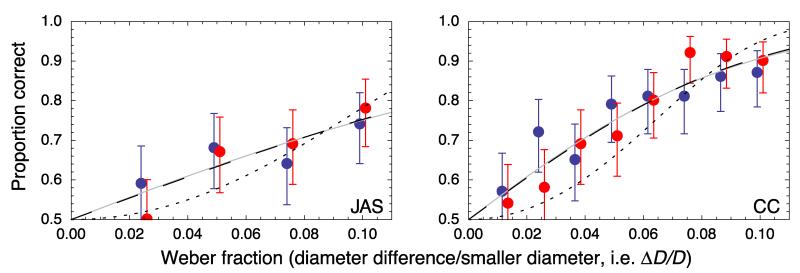
Results appear in Figure 3. Although the two observers clearly differ in their abilities, each achieves an accuracy that seems well described by a single psychometric function of the Weber fraction ΔD/D, where ΔD denotes the difference between the test’s and reference’s diameters.

Figure 3. Psychometric functions for 2AFC size discrimination.

Blue and red symbols illustrate accuracies with ~1.5° and ~3.0° diameters, respectively. Small horizontal nudges have been applied for legibility. Error bars contain 95% confidence intervals. Solid gray curves show maximum likelihood fits of the model: $P\left(C\right)=\Phi \left(\frac{\log \left[\left(\frac{\Delta D}{D}\right)+1\right]}{{\sigma }^{\prime }}\right)$, where P(C) is the probability of a correct response and Φ is the standard normal cumulative distribution function. Dashed curves show the nearly indistinguishable fit of the model: $P\left(C\right)=\Phi \left(\frac{\left[\frac{\Delta D}{D}\right]}{\sigma }\right)$. For JAS, σ = 0.14; for CC, σ = 0.07. Dotted curves show the best—but still poor—fit of the model: $P\left(C\right)=\Phi \left(\frac{\log \left[{\left(\frac{\Delta D}{D}\right)}^2+1\right]}{{\sigma }^{\prime }}\right)$.

When two signals are perturbed by independent, identically distributed (IID) samples of Gaussian noise, accuracy for an ideal discriminator will follow a (cumulative) Gaussian distribution of their difference (Green & Swets, 1966). The smooth curves in Figure 3 suggest that logarithmically transduced circle diameters are consistent with this prediction. To assess goodness of fit, the maximum likelihood of each observer’s data was computed assuming two models: the one-parameter model

$$P\left(C\right)=\Phi \left(\frac{\log \left[\left(\frac{\Delta D}{D}\right)+1\right]}{{\sigma }^{\prime }}\right)$$ (1)

and a more general model having one parameter for each data point (e.g., Watson, 1979). Neither CC’s nor JAS’s data contained sufficient evidence to reject the one-parameter model.²

Having insufficient data to reject alternative models of size discrimination is not, in itself, a strong recommendation for adopting the simple model we propose. Several types of psychometric function³ are too steep to be compatible with an IID sample of Gaussian noise for each signal. For comparison with our simple model, we have adapted a suggestion from Leshowitz, Taub, and Raab (1968) and fit our data with the more general model:

$$P\left(C\right)=\Phi \left(\frac{\log \left[{\left(\frac{\Delta D}{D}\right)}^k+1\right]}{{\sigma }^{\prime }}\right)$$ (2)

If empirical psychometric functions for size discrimination were too steep to be consistent with Gaussian noise, this general model would fit best with k > 1. Nonetheless, we obtained maximum likelihood fits when k = 1.03 for JAS and k = 0.99 for CC.

Although Equation 1 therefore seems to be a good model for size discrimination, values of parameter σ’ can be hard to interpret. On the other hand, parameter σ in Equation 3 is easy to interpret. It is the Weber fraction affording 84% correct, i.e., the just-noticeable Weber fraction (JNWF):

$$P\left(C\right)=\Phi \left(\frac{\left[\frac{\Delta D}{D}\right]}{\sigma }\right)$$ (3)

Although not formally equivalent, dashed curves in Figure 3 show that this alternate formula can produce psychometric functions virtually identical to those produced by Equation 1. The maximum likelihood estimates of the JNWF are 0.14 for JAS and 0.07 for CC.

Discussion

The good agreement between the predictions of signal detection theory and our data allows us to be confident that the visual system effectively perturbs logarithmically transduced circle diameters with IID samples of Gaussian noise when observers attempt to discriminate sizes. An alternative model for the data of Experiment 0 excludes non-linear transduction but includes Gaussian decision noise that increases with circle size. Indeed, estimates of absolute area (Teghtsoonian, 1965) and average area (Chong & Treisman, 2003) both suggest an expansive transduction of circle diameters. To reconcile their results with Weber’s law, the standard deviation of early noise would have to increase linearly with transduced size, and no physical distribution of circle diameters could ensure a Gaussian distribution of noisily transduced sizes. Therefore, we have decided to reserve further attempts to reconcile magnitude estimation with discriminability for future discussion.

Although the performances of our observers (JNWFs around 0.10) were similar to recently reported discriminations of rectangle and oval sizes (Morgan, 2005; Nachmias, 2008), they were significantly worse than earlier reports of line discrimination (Fechner, 1860/1966, pp. 176-197). As yet, it remains unclear whether the shape of our stimuli (i.e., circles rather than lines) is the cause of this discrepancy; however, intuition suggests instead that the brief, parafoveal exposures used here might have been the more critical factor.

It was our intention that observers make their decisions on the basis of circle size, and their performances were similar to previously reported discriminations of rectangle size (Morgan, 2005). Although it remains conceivable that our observers used mechanisms more selective for luminance energy, it seems unlikely. When identically sized lights of different luminance are presented successively, values for the JNWF are considerably higher—between 0.3 and 0.45 (estimated from results in Leshowitz et al., 1968)—than the JNWFs recorded here.

Below, when attempting to create normal distributions of transduced size, we use lognormal distributions of circle diameter.

Experiment 1

To compare efficiencies for visual estimates of different stimulus dimensions, it is important to ensure that measurements are made in similar circumstances. Solomon (2010) measured orientation statistics using demonstrably uncrowded, iso-eccentric arrays containing no more than 8 objects. Adapting his methodology for size statistics, we first attempted to ensure that 8 circles can be placed around fixation in such a way that none interferes with the estimates of another’s size.

Methods

Solomon (2010) used a spatial pre-cue to identify which, in an array of N randomly oriented Gabor patterns, was the one to be remembered and compared with a subsequently displayed Gabor at the same position. For this size experiment, we slightly modified that paradigm to discourage within-array comparisons.

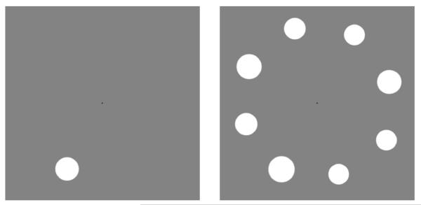
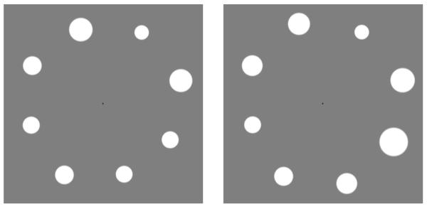
There were two observers, author JAS and AT, a postgraduate student who was naive to the purposes of this experiment. The center of each circle was uniformly distributed between 5.6 and 6.4° from the central fixation spot (see Figure 4).

Figure 4. (Left) First and (right) second displays from a typical trial in Experiment 1.

Observers were required to report whether the circle in the first display was larger or smaller than that circle in the second display having the same azimuth. The various sizes of the other circles were to be ignored.

On each trial of the experiment, two arrays were presented for 0.15 s each. For 1.5 s between these presentations, only the central fixation spot was displayed. The first array contained a single circle at a random azimuth. The second array contained one circle at the same azimuth and N − 1 distractors, equally spaced in azimuth around fixation. The smaller of the two circles sharing an azimuth was nominally the reference; the larger one was the test. Observers were instructed to ignore the distractors and select the display that contained the test. No feedback was given.

For each observer, there were four randomly interleaved conditions (JAS: N ∈ {1, 4, 8, 16}, AT: N ∈ {1, 2, 4, 8}). The angular subtense of the reference and each distractor was sampled from a uniform distribution between 1.5 and 1.9 degrees. At first, JAS performed 8 blocks of 100 trials each, in which the test was either 8 or 10% larger than the reference. Then, both observers performed 8 blocks of 100 trials each, in which the test was either 6 or 12% larger than the reference.

Results

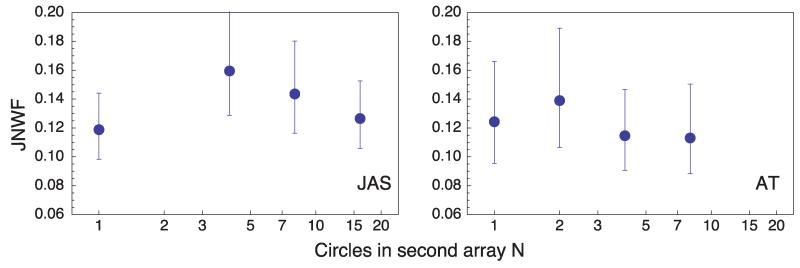
When there was just 1 circle in the second array (i.e., when N = 1), this task was very similar to that used in Experiment 0. As in that experiment, here we used Equation 3 to estimate JNWFs. JAS’s JNWF in Experiment 0 was not significantly different from any of the four JNWFs estimated from his data in Experiment 1 (see Figure 5).

Figure 5. Just-noticeable Weber fractions (JNWFs) for two successively displayed, differently sized circles at ~6° viewing eccentricity.

Error bars contain 95% confidence intervals. There was no systematic effect of the N − 1 distracting circles on JNWF.

The effect of N on JNWF can be assessed for significance using generalized likelihood ratios. Comparison of these ratios to the chi-square distribution having three degrees of freedom (four JNWFs for four Ns versus the null hypothesis of one JNWF for four Ns) suggests a 19% chance of effects this large or larger, even when the null hypothesis is true for JAS. For AT, the probability is 79%. Thus, neither JAS’s nor AT’s data contained sufficient evidence to reject a one-parameter model.

In this experiment, the distance between circles is determined by N. Previous research suggested a decrease in performance once the center-to-center distance between circles decreased beyond about half their viewing eccentricity (Bouma, 1970; van den Berg, Roerdink, & Cornelissen, 2007). There is no hint of this crowding in our results, but note that circle spacing decreased beyond this critical distance only when N = 16.

Discussion

The results of Experiment 1 confirm that observers can discriminate between successively displayed, differently sized circles at ~6° viewing eccentricity, without interference from seven similarly eccentric circles, evenly arrayed around fixation. Circles in this configuration may thus be considered “demonstrably uncrowded,” and thus, we assume that the visual system is not compelled to average their sizes (cf. Parkes, Angelucci, Lund, Solomon, & Morgan, 2001).

Experiment 2

In this experiment, we adopt the external noise perturbation technique to measuring equivalent noise and efficiency (e.g., Pelli, 1990; Solomon, 2010) for use with psychophysical estimates of mean size. External noise perturbation is essential for disentangling efficiency, which describes the fraction of available information used for a statistical summary, from equivalent noise, which limits the precision with which that information can be used. In the absence of external noise, decreases in efficiency become indistinguishable from increases in equivalent noise. Such is the case in typical feature searches (e.g., Morgan, Giora et al., 2008; Palmer, Ames, & Lindsey, 1993), where all of the distractors are identical.

Methods

The same general methods employed in Experiments 0 and 1 were reused in Experiment 2. In this experiment, results were obtained from JAS plus three other experienced psychophysical observers naive to the purposes of this experiment.

On each trial, both displays contained an N-circle array (N ∈ {1, 2, 4, 8}; see Figure 6). One of these arrays was nominally the reference. Diameters in this array were randomly selected from the lognormal distribution $\ln \mathcal{N}(\ln D,{\sigma }_{\mathrm{C}}^2)$, having a “baseline” diameter D that was randomly selected from the interval [1.0°, 1.2°]. Diameters in the N-circle, “test” display were randomly selected from the lognormal distribution $\ln \mathcal{N}\left[\ln \right(D+\Delta D),{\sigma }_{\mathrm{C}}^2]$, whose baseline diameter (D + ΔD) was greater than that of the reference display. The same value of “stimulus SD” σ_C was used for both displays. Note that σ_C is not the standard deviation of circle diameters; it is the standard deviation of discriminable sizes following logarithmic transduction. For JAS, σ_C ∈ {0.025, 0.050, 0.10, 0.20}, and for ZC and KM, σ_C ∈ {0.015, 0.030, 0.060, 0.120}. The reference and test displays were presented in random order. Observers’ instructions were “If the average in the first array was larger, press c. If the average in the second array was larger, press m.” No feedback was given.

Figure 6. The two displays from a typical trial in Experiment 2.

Observers were required to report which display had the larger average size.

The Weber fraction (ΔD/D) was determined by one of 16 randomly interleaved QUEST staircases (Watson & Pelli, 1983), one for each combination of N and Σ_C. As in Solomon (2010), trials with large Weber fractions were introduced to measure lapses of attention. On these trials, which had a stationary probability of occurrence of 0.1, the staircases were ignored and (ΔD/D) was set to 0.4. After one block of 80 practice trials, each observer completed 16 blocks of 80 trials each. New staircases were begun after the fourth, eighth, and twelfth blocks.

Results

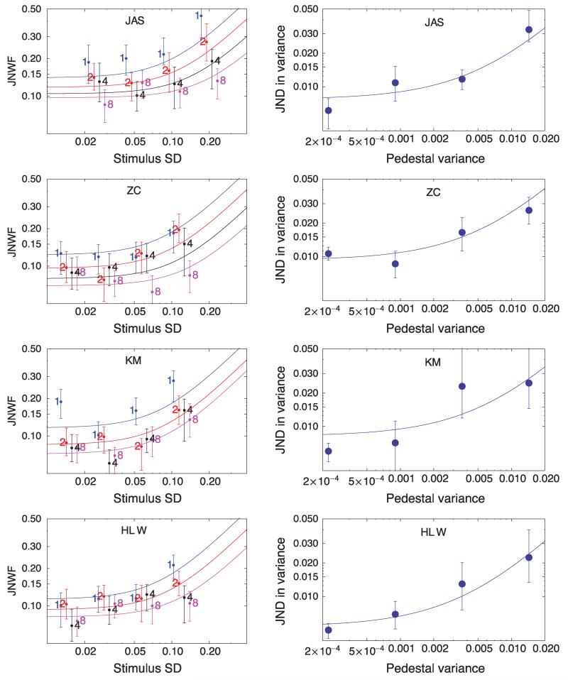
Considered en masse, just-noticeable Weber fractions for JAS were generally higher than those of KM and certainly higher than those of ZC and HLW. However, all three observers suffered an elevation of JNWF when stimulus SD was greatest, and all three observers enjoyed a reduction of JNWFs when the number of circles per array increased from 1 to 8 (see Figure 7).

Figure 7. JNWFs between the (geometric) mean orientations (left) and just-noticeable differences (JNDs) in variance (right) of two successively displayed, uncrowded circle arrays.

SDs and variances, respectively, refer to parameters σ_C and ${\sigma }_{\mathrm{C}}^2$ of the lognormal distributions from which circle diameters were drawn. Numerals denote N, the number of circles per array. They have been nudged horizontally for better legibility. Error bars contain 95% confidence intervals. Blue, red, black, and magenta curves illustrate the best 3-parameter fit to the data on the left for N = 1, N = 2, N = 4, and N = 8, respectively. (Fits to N = 4 and N = 8 were identical for subject KM. They were also identical for HLW.) Simultaneous fits for variance discrimination, where N = 8, are shown on the right.

Modeling

Human observers cannot perform visual calculations of statistics without making errors. As diagrammed in Figure 1, early noise can perturb each estimate of diameter, and late noise can perturb the calculations themselves. Moreover, these calculations may be inefficient, with human observers effectively using only M_mean of the N circles available in each display. Accuracy for this noisy, inefficient (but otherwise ideal) observer is given by the following formula:

$$P\left(C\right)=\frac{1}{2}+\left(\frac{1}{2}-\delta \right)\Phi \left[\frac{\ln (1+\Delta D∕D)}{\sqrt{{\sigma }_{\mathrm{L}}^2+2({\sigma }_{\mathrm{E}}^2+{\sigma }_{\mathrm{C}}^2)∕M_{\text{mean}}}}\right]$$ (4)

where σ_C is a parameter of the lognormal distributions from which circle diameters were drawn (see Methods section) and M_mean, σ_E, and σ_L are free parameters. M_mean represents the number of circles observers use when calculating the mean of each array and M_mean ≤ N. σ_E and σ_L represent the standard deviations of the early and late noises, respectively. Psychometric ceiling 1 − δ was set to reflect the empirical lapse rates: δ = 0.040 for JAS, δ = 0.026 for ZC, δ = 0.012 for KM, and δ = 0.006 for HLW. NB: The fraction in Equation 4 has a 2 inside the square root in its denominator because of the 2AFC paradigm; decisions are necessarily affected by the noise in both arrays.

Equation 4 fit the data from JAS, ZC, and HLW with maximum likelihood when M_mean = N, i.e., when these three observers were operating at 100% efficiency. However, fits with M_mean = min{7, N} were almost as good. On the basis of their data from Experiment 2, hypotheses of the form M_mean = min{M_max, N} can be rejected with 95% confidence only when M_max ≤ 3. In other words, we can be reasonably confident that JAS, ZC, and HLW can use more than 3 circles when estimating mean size in a 0.15-s glimpse.

Observer KM was less efficient than JAS, ZC, and HLW. Equation 4 fit his data with maximum likelihood when M_mean = min{3, N}. Here, it must be noted that, unless stated otherwise, our fits were not constrained such that M_mean = min{M_max, N}. Nonetheless, the maximum likelihood fit of Equation 4 to each observer’s data was consistent with this constraint. In KM’s case, fits adhering to this constraint were significantly worse both when M_max ≤ 2 and when M_max ≥ 5. Thus, for example, we can be reasonably confident that KM effectively uses only 3 or 4 circles when attempting to estimate the mean size in 4- and 8-circle arrays.

Various other (null) hypotheses regarding the noisy, inefficient observer were tested. The only one that could be rejected at the 0.05 level on the basis of each observer’s data was σ_E = 0. ZC’s data also contained sufficient evidence for rejecting the hypothesis that σ_L = 0.

Discussion

Myczek and Simons (2008) reviewed contemporary evidence for inefficient comparisons of mean size and concluded that there was no compelling evidence for computations based on more than one or two items in any given set of circles. Results from our Experiment 2 qualify this conclusion, in the sense that they now provide compelling evidence that some observers can use at least 3 circles in rapid estimates of average size.

Experiment 3

Solomon (2010) wondered whether the greater efficiency for discriminations of orientation variance than for discriminations of mean orientation might be due to the cyclical nature of orientation. This question is addressed here, where we gather data on the discrimination of size variances for comparison with Experiment 2’s discriminations of mean size.

Methods

The same general methods employed in Experiment 2 were reused in Experiment 3, with the following exceptions. Only arrays of size N = 8 were used in this experiment. As before, the diameters in each array were selected from a lognormal distribution. However, in this experiment, the baseline diameters for test and reference (D_t and D_r) were independently selected from the interval (1.0°, 1.2°). Reference diameters were drawn at random from the lognormal distribution $\ln \mathcal{N}(\ln D_{\mathrm{r}},{\sigma }_{\mathrm{C}}^2)$, where “pedestal variance” ${\sigma }_{\mathrm{C}}^2$ was a member of the set {0.015², 0.030², 0.060², 0.12²}. Again, note that ${\sigma }_{\mathrm{C}}^2$ is not the variance of circle diameters; it is the variance of sizes following a logarithmic transduction, i.e., the sizes available to the observer for further, statistical processing.

Test diameters were drawn at random from the log-normal distribution $\ln \mathcal{N}(\ln D_{\mathrm{t}},{\sigma }_{\mathrm{C}}^2+\Delta {\sigma }_{\mathrm{C}}^2)$. Two QUEST staircases were randomly interleaved for each pedestal variance to determine $\Delta {\sigma }_{\mathrm{C}}^2$, one converging on an accuracy of P(C) = 0.67, the other converging on an accuracy of P(C) = 0.84. As in previous studies (Morgan, Chubb, & Solomon, 2008; Solomon, 2010), here we adopt the atheoretical approach to defining the just-noticeable difference (JND) between variances as the scale α of a cumulative Weibull distribution:

$$P\left(C\right)=\frac{1}{2}+\left(\frac{1}{2}-\delta \right)\left(1-\exp \left[-{\left(\frac{\Delta {\sigma }_{\mathrm{C}}^2}{\alpha }\right)}^{\beta }\right]\right)$$ (5)

Psychometric functions of this form were also implicitly assumed by QUEST, using a lapse rate (δ = 0.01) and slope (β = 20) that were determined in a pilot experiment. Individual estimates of lapse rate were facilitated by QUEST with probability of 0.10 on every trial and setting $\Delta {\sigma }_{\mathrm{C}}^2=0.05$.

The observer’s task was to select the test. To ensure ZC, KM, and HLW understood the task, each was told, “It may be hard to define variance, but it’s easy to understand its opposite. That’s when all the circles have the same size. Your task is to select the display in which the circle sizes are most different to each other.” After one block of 110 practice trials, ZC, KM, and HLW each completed 8 blocks of 110 trials each. JAS completed 16 blocks. New staircases were begun after the fourth, eighth, and twelfth blocks.

Results

Data from all four observers exhibit an upward trend of JND with pedestal variance (see Figure 7). A simple linear regression of the 16 JNDs against their corresponding pedestal values suggests a highly significant correlation: p < 10⁻⁵.

Modeling

To establish efficiencies for discriminating size variances, we must compare human performances with the performance of the ideal discriminator. The ideal discriminator computes the sample variance in each interval and selects the interval having the greatest sample variance. As described above, our circles have been selected to form a Gaussian distribution of transduced sizes. Therefore, a proportion of their sample variances will follow the chi-square distribution, and the ratio of two such sample variances will follow the F distribution. To assess human performances, here we adapt previous derivations of inefficient, noisy versions of the ideal discriminator for 2AFC variance discrimination (Morgan, Chubb et al., 2008;⁴ Solomon, 2010) to the dimension of size. This adaptation requires the straightforward substitution of logarithmically transduced circle diameters for spatial orientations:

$$P\left(C\right)=(1-2\delta )F\left(\frac{{\sigma }_{\mathrm{C}}^2+\Delta {\sigma }_{\mathrm{C}}^2+{\sigma }_{\mathrm{E}}^2}{{\sigma }_{\mathrm{C}}^2+{\sigma }_{\mathrm{E}}^2}\right)+\delta$$ (6)

where F is the (cumulative) F distribution, with degrees of freedom M_var − 1 and M_var − 1. As in Equation 4, here M_var represents the number of circles observers use when calculating the variance of each array and M_var ≤ N. σ_E represents the standard deviation of the early noise, and δ is the lapse rate, empirically determined from trials in which ${\sigma }_{\mathrm{C}}^2\le {0.030}^2$ and $\Delta {\sigma }_{\mathrm{C}}^2=0.05$ for JAS, δ = 0.039 for ZC, δ = 0.024 for KM, and δ = 0.001 for HLW. (Small non-zero lapse rates such as this latter value are not only computationally convenient but also, at least, seem to be a more sensible approximation to observer capability than a lapse rate of zero, which is what HLW’s data actually contain.)

Note that this formula does not include a term for late noise, which could further perturb estimates of sample variance. Were such a term added, its distribution would have to be convolved with the F distribution. Obtaining maximum likelihood fits with such a complicated psychometric function would not only be computationally intractable but also necessarily overfit the data from Experiment 3, which used just one array size, and thus cannot simultaneously constrain the variances of early and late noises. Consequently, readers are urged to note the implications of non-negligible late noise for variance discriminations. Specifically, the presence of such noise would imply that our estimates of σ_E (below) are too high, and thus, the real ratio of σ_L/σ_E for mean discriminations may be somewhat higher than ratios calculated from those estimates.

The availability of mean discrimination data and variance discrimination data from the same observers in otherwise identical conditions affords a statistical evaluation of several hypotheses within the framework of an inefficient, noisy observer. Adopting the constraint satisfied by maximum likelihood fits to each observer’s data in Experiment 2 (i.e., M_mean = min{M_max, N}, see above), all responses in both Experiments 2 and 3 can be simultaneously fit with a four-parameter model. Maximum likelihood fits are shown in Figure 7. For JAS, σ_E = 0.077, σ_L = 0.089, M_max = 8, and M_var = 6; for ZC, σ_E = 0.077, σ_L = 0.058, M_max = 8, and M_var = 5; for KM, σ_E = 0.079, σ_L = 0.031, M_max = 3, and M_var = 6; and for HLW, σ_E = 0.064, σ_L = 0.068, M_max = 4, and M_var = 6.

As previously noted, each observer’s data contain sufficient evidence to reject the hypothesis that σ_E = 0. Furthermore, when data from Experiments 2 and 3 are combined, each observer’s data also contain sufficient evidence to reject the hypothesis that σ_L = 0. Finally, the 95% confidence interval on M_var for all four observers is (5, 8).

One further hypothesis, which could not be rejected on the basis of any observer’s data, is that M_max = M_var. In other words, and in contrast to the results obtained in experiments investigating efficiencies of summary statistics for spatial orientation (Solomon, 2010), our observers seem to have been no more efficient comparing size variances than they were at comparing mean sizes.

Discussion

The data show that our ability to form statistical summaries of size is qualitatively different from our previously reported (Solomon, 2010) ability to form statistical summaries of orientation. Although efficiencies for mean size discrimination do differ from individual to individual, in none of the individuals we tested was this efficiency significantly lower than that for size variance discrimination. On the other hand, all of Solomon’s (2010) observers exhibited significantly lower efficiencies for mean orientation discrimination than for orientation variance discrimination.

General discussion

Our current data do not contain sufficient evidence for us to confidently reject the proposal (Myczek & Simons, 2008) that statistical estimates may be approximated using heuristics based on the range of visible values rather than their mean or variance per se. Regardless of dimension, a noiseless observer whose decisions were based merely on the extrema of 8 values sampled from a Gaussian distribution would produce efficiencies of approximately 62% when discriminating between two means and 91% when discriminating between two variances (Solomon, 2010). These efficiencies fall within the 95% confidence intervals inferred from each of our observers’ data.

Of course, decisions based on the extrema of visual sets can be made only after those extrema have been identified and that can only happen after each item undergoes some form of analysis. Thus, we can conclude that the visual system is quite capable of quickly producing summary statistics of size. The formulas it uses for calculating those statistics might differ from those used by your computer, but its estimates are pretty good nonetheless.

The current study was designed to reveal whether mean discriminations would have lower precision than variance discriminations for size, a non-cyclical dimension. The answer is yes. Just like Solomon’s (2010) investigation of orientation statistics, our results with size statistics contain evidence for a non-negligible source of late noise that limits mean discriminations but not variance discriminations.

References

- Ariely D. Seeing sets: Representation by statistical properties. Psychological Science. 2001;12:157–162. doi: 10.1111/1467-9280.00327. [DOI] [PubMed] [Google Scholar]
- Ariely D. Better than average? When can we say that subsampling of items is better than statistical summary representations? Perception and Psychophysics. 2008;70:1325–1326. doi: 10.3758/PP.70.7.1325. [DOI] [PubMed] [Google Scholar]
- Bouma H. Interaction effects in parafoveal letter recognition. Nature. 1970;226:177–178. doi: 10.1038/226177a0. [DOI] [PubMed] [Google Scholar]
- Brainard DH. The psychophysics toolbox. Spatial Vision. 1997;10:433–436. [PubMed] [Google Scholar]
- Chong SC, Joo SJ, Emmanouil T-A, Treisman A. Statistical processing: Not so implausible. Perception and Psychophysics. 2008;70:1327–1334. doi: 10.3758/PP.70.7.1327. [DOI] [PubMed] [Google Scholar]
- Chong SC, Treisman A. Representation of statistical properties. Vision Research. 2003;43:393–404. doi: 10.1016/s0042-6989(02)00596-5. [DOI] [PubMed] [Google Scholar]
- Chong SC, Treisman A. Attentional spread in the statistical processing of visual displays. Perception and Psychophysics. 2005a;67:1–13. doi: 10.3758/bf03195009. [DOI] [PubMed] [Google Scholar]
- Chong SC, Treisman A. Statistical processing: Computing the average size in perceptual groups. Vision Research. 2005b;45:891–900. doi: 10.1016/j.visres.2004.10.004. [DOI] [PubMed] [Google Scholar]
- Dakin SC. Information limit on the spatial integration of local orientation signals. Journal of the Optical Society of America. A, Optics, image science, and vision. 2001;18:1016–1026. doi: 10.1364/josaa.18.001016. [DOI] [PubMed] [Google Scholar]
- Fechner G, Howes DH, Boring EG. Elemente der Psychophysik [Elements of psychophysics (vol. 1)] Rinehart and Winston; Holt: 1966. Original work published 1860. [Google Scholar]
- Fisher RA. Statistical methods for research workers. Oliver and Boyd; Edinburgh, UK and London: 1925. [Google Scholar]
- Green DM. Psychoacoustics and detection theory. Journal of the Acoustical Society of America. 1960;32:1189–1203. [Google Scholar]
- Green DM, Swets JA. Signal detection theory and psychophysics. Wiley; New York: 1966. [Google Scholar]
- Heeley DW, Buchanan-Smith HM, Cromwell JA, Wright JS. The oblique effect in orientation acuity. Vision Research. 1997;37:235–242. doi: 10.1016/s0042-6989(96)00097-1. [DOI] [PubMed] [Google Scholar]
- Leshowitz B, Taub HB, Raab DH. Visual detection of signals in the presence of continuous and pulsed backgrounds. Perception and Psychophysics. 1968;4:207–213. [Google Scholar]
- Mood AM, Graybill FA, Boes DC. Introduction to the theory of Statistics. McGraw-Hill; 1974. [Google Scholar]
- Morgan M, Chubb C, Solomon JA. A ‘dipper’ function for texture discrimination based on orientation variance. Journal of Vision. 2008;8(11):9, 1–8. doi: 10.1167/8.11.9. http://www.journalofvision.org/content/8/11/9. doi:10.1167/8.11.9. [DOI] [PMC free article] [PubMed] [Google Scholar]
- Morgan MJ. The visual computation of 2-D area by human observers. Vision Research. 2005;45:2564–2570. doi: 10.1016/j.visres.2005.04.004. [DOI] [PubMed] [Google Scholar]
- Morgan MJ, Giora E, Solomon JA. A single “stopwatch” for duration estimation, A single “ruler” for size. Journal of Vision. 2008;8(2):14, 1–8. doi: 10.1167/8.2.14. http://www.journalofvision.org/content/8/2/14. doi:10.1167/8.2.14. [DOI] [PMC free article] [PubMed] [Google Scholar]
- Myczek K, Simons DJ. Better than average: Alternatives to statistical summary representations in rapid judgments of average size. Perception and Psychophysics. 2008;70:772–788. doi: 10.3758/pp.70.5.772. [DOI] [PubMed] [Google Scholar]
- Nachmias J. Judging spatial properties of simple figures. Vision Research. 2008;48:1290–1296. doi: 10.1016/j.visres.2008.02.024. [DOI] [PubMed] [Google Scholar]
- Palmer J, Ames CT, Lindsey DT. Measuring the effect of attention on simple visual search. Journal of Experimental Psychology. 1993;19:108–130. doi: 10.1037//0096-1523.19.1.108. [DOI] [PubMed] [Google Scholar]
- Parkes L, Lund J, Angelucci A, Solomon J, Morgan M. Compulsory averaging of crowded orientation signals in human vision. Nature Neuroscience. 2001;4:739–744. doi: 10.1038/89532. [DOI] [PubMed] [Google Scholar]
- Pelli DG. The quantum efficiency of vision. In: Blakemore C, editor. Vision: Coding and efficiency. Cambridge University Press; Cambridge, UK: 1990. pp. 3–24. [Google Scholar]
- Pelli DG. The VideoToolbox software for visual psychophysics: Transforming numbers into movies. Spatial Vision. 1997;10:437–442. [PubMed] [Google Scholar]
- Solomon JA. Visual discrimination of orientation statistics in crowded and uncrowded arrays. Journal of Vision. 2010;10(14):19, 1–16. doi: 10.1167/10.14.19. http://www.journalofvision.org/content/10/14/19. doi:10.1167/10.14.19. [DOI] [PubMed] [Google Scholar]
- Teghtsoonian M. The judgment of size. American Journal of Psychology. 1965;78:392–402. [PubMed] [Google Scholar]
- Tomassini A, Morgan MJ, Solomon JA. Orientation uncertainty reduces perceived obliquity. Vision Research. 2010;50:541–547. doi: 10.1016/j.visres.2009.12.005. [DOI] [PubMed] [Google Scholar]
- van den Berg R, Roerdink JB, Cornelissen FW. On the generality of crowding: Visual crowding in size, saturation, and hue compared to orientation. Journal of Vision. 2007;7(2):14.1–11. doi: 10.1167/7.2.14. http://www.journalofvision.org/content/7/2/14. doi:10.1167/7.2.14. [DOI] [PubMed] [Google Scholar]
- Watson AB. Probability summation over time. Vision Research. 1979;19:515–522. doi: 10.1016/0042-6989(79)90136-6. [DOI] [PubMed] [Google Scholar]
- Watson AB, Pelli DG. QUEST: A Bayesian adaptive psychometric method. Perception and Psycho-physics. 1983;33:113–120. doi: 10.3758/bf03202828. [DOI] [PubMed] [Google Scholar]
- Weber EH. Der Tastsinn und das Gemeingefuhl (p. 559); quoted in Ross, H. E., & Murray, D. J. (1996). E. H. Weber on the tactile senses (p. 211) Erlbaum, Taylor & Francis; Hove, UK: 1851. [Google Scholar]