Abstract
Due to the wide applications, spreading processes on complex networks have been intensively studied. However, one of the most fundamental problems has not yet been well addressed: predicting the evolution of spreading based on a given snapshot of the propagation on networks. With this problem solved, one can accelerate or slow down the spreading in advance if the predicted propagation result is narrower or wider than expected. In this paper, we propose an iterative algorithm to estimate the infection probability of the spreading process and then apply it to a mean-field approach to predict the spreading coverage. The validation of the method is performed in both artificial and real networks. The results show that our method is accurate in both infection probability estimation and spreading coverage prediction.
Many complex systems can be characterized by networks in which nodes represent the individuals and edges represent the interactions. Examples include citation networks1,2, communication networks3, transportation networks4, cyber networks5, financial networks6, just to name a few. The study of complex networks has therefore become a common focus of many branches of science. So far, great efforts have been made to understand and predict the evolution of networks. For instance, link prediction intends to identify which pair of nodes will be connected in the future7,8. Trend prediction aims at predicting the future degree of nodes2,9. However, most of the related works focus on the structural aspect of networks. Even though dynamical processes commonly take place in real networks10, the prediction of the evolution of dynamics on networks has been seriously overlooked.
Spreading is an important kind of dynamics which has been applied to model many real processes on network such as spreading of disease11,12,13,14, propagation of news and rumors15,16,17,18, cascading failure of power grid19, and so on. In this paper, we focus on predicting the evolution of spreading. Solving this problem is very meaningful from the practical point of view. In the context of disease spreading, one can immunize nodes and links in advance to prevent the virus from covering the whole network if the predicted coverage of the spreading is very wide13,20,21,22,23,24. On the other hand, the propagation of some important information can be accelerated by adding more spreading seeds beforehand if the predicted coverage of the propagation is very narrow25,26,27,28,29,30.
In the cases where prediction is needed, the known information of the spreading process is usually very limited, especially in the early stage of the spreading31,32. Similar to the ref. 33, we assume in this paper that only a snapshot of the spreading result is given. In the literature, the prediction of spreading is mostly based on the time series analysis34. The closest studies based on spreading snapshot are refs. 35, 36 where the observed snapshot is used to identify the initial spreader of a certain disease or information. In the prediction of spreading, the essential problem is how to accurately estimate the infection probability from the observed snapshot. One can consider the most straightforward method in which the infection probability is estimated based on each infected node i as μi = mi/Mi where mi and Mi are respectively the infected number and the total number of i's neighbors. By averaging μi over all the infected nodes in the network, one can estimate the infection probability of the spreading. This method is referred as the “benchmark” method in this paper. However, the benchmark method may lead to serious overestimation of the infection probability. As this method doesn't distinguish which node spreads the virus to the infected node, each infected node may be used more than once in μi = mi/Mi for different i (see the illustration in Fig. 1).
Figure 1. A snapshot of the spreading result in a toy network.
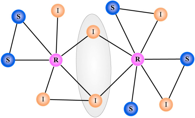
The blue nodes are susceptible (marked by S), yellow nodes are infected (marked by I) and pink nodes are recovered (marked by R). Since each node inside the shade ellipse is connecting to two R nodes, one cannot distinguish which R node actually infected these two I nodes in the previous step. In the benchmark method, these two I nodes will be used when estimating the infection probability based on each R node, which finally leads to an overestimation of the infection probability.
To solve this problem, we develop an iterative algorithm for estimating the infection probability (IAIP for short) in which the problem of multiple use of the infected nodes is avoided. We validate the IAIP by simulating the Susceptible-Infected-Removed (SIR) model37 in both artificial and real networks. The results show that our method can significantly outperform the benchmark method. Moreover, we study the case in which the iterative process is removed from our method (denoted as IAIP0). The results show that IAIP0 performs much less effectively than IAIP, indicating the crucial role of the iterative process. When the obtained infection probability is used in predicting the future spreading coverage, a much more accurate prediction can be achieved by using IAIP.
Results
We consider a network with N nodes and E links. The network is represented by an adjacency matrix A, where Aij = 1 if there is a link between node i and j, and Aij = 0 otherwise. To simulate the spreading process on networks, we employ the Susceptible-Infected-Removed (SIR) model37. In a network, we randomly select one node as the initial spreader. The virus from this node will infect each of this node's susceptible neighbors with probability μ, namely the infection probability. After infecting neighbors, the node will immediately become recovered (i.e., the recovering probability is 1). The new infected nodes in next step will infect their neighbors as the initial node. The spreading will be ended when there is no more infected node in the network. If it is not specially stated, we take the snapshot after five steps of spreading from the initial node as the known information.
Epidemic spreading is a stochastic process. Given an infection probability and an initial infected node, the spreading results can vary significantly in different realizations. An observed snapshot may be corresponding to many different μ values. Therefore, one cannot use the deterministic models to exactly infer the μ value from the spreading snapshot. In this paper, we propose an iterative method to infer the μ value. Though the inference is not exact, we will show below the expected value of the obtained μ is very close to the real infection probability, with a relatively small dispersion.
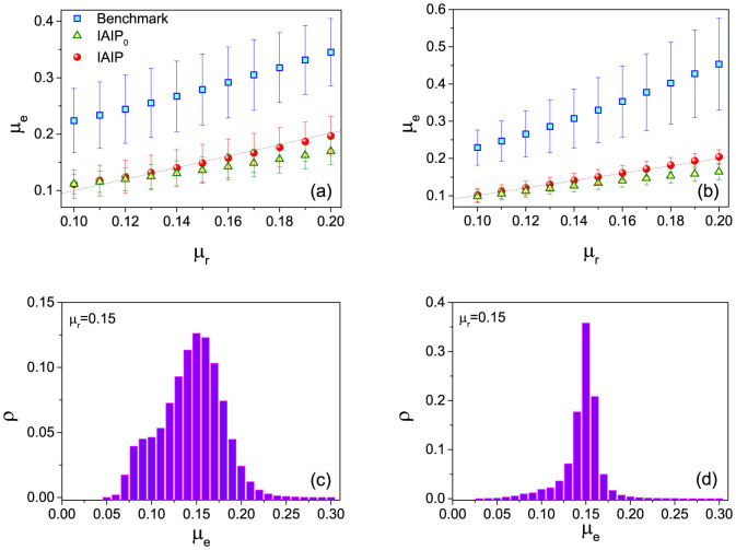
We first test the IAIP (see the Method section for description) in artificial networks: Watts-Strogatz (WS) networks38 and Barabási-Albert (BA) networks39. In Fig. 2(a) and (b), we show the estimated infection probability from the benchmark, IAIP0 and IAIP methods μe as a function of the true infection probability μr. Obviously, if a method can accurately estimate the infection probability, the curve of this method in Fig. 2(a) and (b) should overlap well with μe = μr. One can immediately notice that the curve of the IAIP locates around μe = μr while the curve of the benchmark method is significantly higher than that, indicating a serious overestimation of the infection probability in the benchmark method. Moreover, without the iterative process the curve of the IAIP0 is lower than μe = μr. In Fig. 2(c) and (d), we fix an infection probability and investigate the disparity of μe from the IAIP under different choice of initial spreaders (each node is selected once as the initial spreader). The distribution of μe is rather narrow with 〈μe〉 ≈ μr, indicating the stable performance of the IAIP. Moreover, the deviation of μe is much smaller in BA networks than that in WS networks. We thus conclude that IAIP performs more stably in the networks with heterogenous degree distribution which can be widely observed in real systems.
Figure 2.
The estimated infection probability μe from different methods as a function of the true infection probability μr in (a) WS and (b) BA networks. μe = μr is plotted with dashed lines to guide eyes. The distributions of μe in (c) WS and (d) BA networks are shown. The error bars in (a)(b) and the distribution in (c)(d) are obtained by estimating the infection probability μe under 100 spreading realizations from each node in the network. The network parameters are N = 4000, 〈k〉 = 10, p = 0.4 for WS networks, and N = 4000, 〈k〉 = 10 for BA networks.
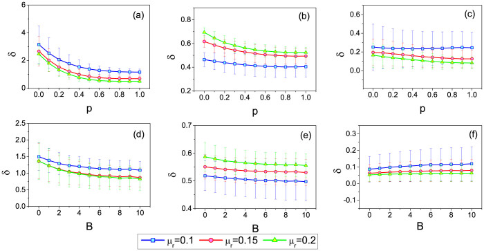
In order to quantify the accuracy of the infection probability estimation, we define an error rate metric as  . According to the definition, a smaller δ indicates a more accurate estimation. We then investigate how the network topology affects the value of δ. For WS networks, we study the effect of the rewiring parameter p on δ. For BA network, we consider a variant of it in which each new node i connect to the existing node j with probability pi = (ki + B)/Σj(kj + B)40,41. This modified model allows a selection of the exponent of the power-law scaling in the degree distribution p(k) ~ k−γ, with γ = 3 + B/m in the thermodynamic limit. With this network, we study the effect of B on δ. Related results on the WS and the modified BA networks are shown in Fig. 3. By comparing fig. 3(a)(b)(c), one can immediately see that when p is small, δ of IAIP can be approximately 10 times smaller than that in the benchmark method and 3 times smaller than that in IAIP0. Though δ in both methods decreases with p, this effect is much stronger in the benchmark method. The local clustering effect of the WS network is destroyed when p is large, which makes the infected nodes adjacent to each other less frequently. The problem of multiple use of the infected nodes in μi = mi/Mi becomes less serious in the benchmark method accordingly. However, note that in real social networks the clustering coefficient is usually very high, which indicates a low accuracy of the benchmark method in real applications. Fig. 3(d)(e)(f) show the results of the benchmark, IAIP0, IAIP methods on the modified BA networks. One can see that IAIP still enjoys the smallest δ. Moreover, δ of the benchmark method decreases with B in the modified BA networks. On the contrary, the performance of the IAIP method doesn't strongly depend on the network structure, indicating the high reliability of the IAIP method.
Figure 3.
The dependence of the error rate δ on p in WS networks for the (a) benchmark, (b) IAIP0 and (c) IAIP methods. The dependence of the error rate δ on B in the modified BA networks for the (d) benchmark, (e) IAIP0 and (f) IAIP methods. In all artificial networks, the network size is N = 4000 and average degree is 〈k〉 = 10. The mean values and error bars are obtained by estimating the infection probability μe under 100 spreading realizations from each node in the network.
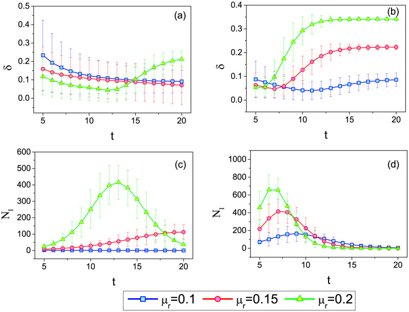
In all the analysis above, we consider the spreading results at t = 5 as the observed snapshot. As in real cases the snapshot at hand may be from different spreading stage, it is therefore interesting to study the relation between δ and t. In Fig. 4, we report the dependence of δ on t. Fig. 4(a) and (b) are the results of the IAIP in WS and BA networks, respectively. One can see that there is an optimal δ when tuning t. In order to understand this phenomenon, we show the number of infected nodes NI versus the spreading step t in Fig. 4(c) and (d). Consistent with previous results in the literature, we observe here that NI first increases then decreases with t. Interestingly, the optimal t* for δ is the same as the t where NI achieves its maximum. When t is large, NI is very small and the spreading is more or less at its final stage. In this situation δ of IAIP is relatively high. However, this is not a problem in practice since usually we only need to predict the future spreading coverage when t is small. We also check the dependence of δ on t in the benchmark method. We observe that δ quickly increases with t. This is because the risk of overestimation of the infection probability becomes more serious when the virus covers a large part of the network.
Figure 4.
The dependence of the estimation accuracy δ of the IAIP on the time of the snapshot t in (a) WS and (b) BA networks. (c) and (d) are respectively the number of infected nodes NI versus the spreading step t in WS and BA networks. The network parameters are the same as those in Fig. 2. The mean values and error bars are obtained by simulating 100 spreading realizations from each node in the network.
We further test the IAIP method in some large-scale real networks. Both undirected and directed networks are considered: Cond-mat (undirected scientific collaboration network)42, Youtube (undirected online users friendship network)43, EmailEU (directed email communication network)44, Delicious (directed online user friendship network)45. In Cond-mat, EmailEU and Delicious, the real infection probability is set as μr = 0.2, and in Youtube, it is set as μr = 0.05. In each realization, we randomly pick a node from the network and apply the benchmark, IAIP0 and IAIP methods on the spreading snapshot at t = 5. We calculate the error rate δ after the μe is obtained. The mean error rate 〈δ〉 of each method is finally obtained by randomly selecting 1000 initial nodes and simulating 100 spreading realizations from each of these initial nodes. Results on the real networks are reported in table 1. Consistent with the results in artificial networks, the IAIP method enjoys a much smaller error rate than the IAIP0 and benchmark methods.
Table 1. Basic structural properties (network size N, edge number E) and the mean error rate 〈δ〉 of the benchmark, IAIP0 and IAIP methods in real networks.
| Network | N | E | 〈δ〉benchmark |  |
〈δ〉IAIP |
|---|---|---|---|---|---|
| Cond-mat | 27,519 | 116,181 | 2.0678 | 0.3513 | 0.0957 |
| EmailEU | 265,214 | 418,956 | 3.3186 | 0.3999 | 0.0245 |
| Delicious | 582,377 | 1,679,090 | 1.4066 | 0.3519 | 0.1465 |
| Youtube | 1,134,890 | 2,987,624 | 8.2508 | 0.2479 | 0.0878 |
Accurately estimating μ can lead to many applications, here we are mainly interested in predicting the spreading coverage based on the μe. At the mean-field level, the dynamics of the SIR model in complex networks can be described by differential equations as46
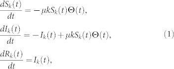 |
where Sk(t), Ik(t) and Rk(t) are the density of susceptible, infected, and removed nodes of degree k at time t, respectively. According to the definition, Sk(t) + Ik(t) + Rk(t) = 1. The factor Θ(t) represents the probability that any given link points to an infected node and is given by
 |
where P(k) is the degree distribution and 〈k〉 is the average degree of the network. In order to predict the coverage at time t + 1, one can follow
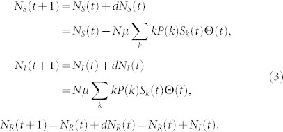 |
The equation (3) can be iteratively used to predict the spreading coverage in longer term, namely t + m. We refer this method as the mean-field (MF) prediction method. From equation (3), one can see that the essential parameter determining the prediction accuracy is μ. We thus study the prediction accuracy when μe of the benchmark, IAIP0 and IAIP methods are used. The results in Fig. 5 show that the mean-field predictors with both IAIP0 and IAIP methods are close to the true evolution.
Figure 5. The predicted and real evolution of NI + NR in (a) WS and (b) BA networks.
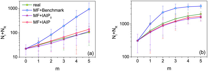
The real infection probability is set as μr = 0.15. m is the number of spreading steps after the observed snapshot. The network parameters are the same as those in Fig. 2. The mean values and error bars are obtained by predicting the future spreading coverage under 100 spreading realizations from each node in the network.
Besides the mean-field model, we have considered some more realistic models, such as the pair approximation model47,48,49 and moment closure approximation model50. The main difference between the mean-field and pair approximation is that the former (latter) approximates high-order moments in term of first (second) order ones. For the moment closure approximation, it can incorporate the structure of the network into the model and allows for the definition of the triples in terms of pairs. We applied the estimated μ value to the pair approximation models47,48, and find consistent results to the mean-filed case, i.e., the prediction based on IAIP0 and IAIP methods is very close to the true evolution.
Discussion
Prediction in complex networks has always been an important research topic. Though many related researches have been done, most of them focus on structural aspects such as link prediction and node popularity prediction. The problems of estimating infection probability from a given spreading snapshot and accordingly predicting the spreading results are very important, with many potential applications in real systems. However, little has been done in this research direction. In this paper, we first design an iterative algorithm to estimate the spreading infection probability from an observed spreading snapshot. The simulation in both artificial and real networks shows that our method enjoys a high accuracy in estimating the spreading infection probability. Finally, the estimated infection probability is applied to a mean-field method for predicting the evolution of the spreading coverage.
In this paper, we consider the basic SIR model in which the recovery probability is set as β = 1. The infectious period is one time-step. We also investigate the more complicated case where β < 1. Our model cannot be directly applied to estimate the parameter β. However, in this case the μ value obtained from our method is actually corresponding to the effective infection probability, i.e. μeff = μ/β. We observe that the estimation of μeff becomes less accurate when β is smaller. In fact, the situation of β < 1 is very complicated, which requires some new method directly estimating μ and β. Related research in this direction is an interesting extension in the future.
Some more issues remain still open. In this paper, we focus on the SIR model, it would be interesting to examine the proposed iterative method in some other spreading models such as SI, SIS. Moreover, the mean-field prediction method in this paper can only predict the width of the spreading. A more interesting and important issue would be predicting which nodes will be infected in the future. Besides spreading, there are many other dynamical processes on networks such as synchronization and percolation51,52. We hope the method and results in this paper can inspire some prediction methods for other dynamical processes.
Methods
We now describe the iterative algorithm for estimating the infection probability (the IAIP method). In a snapshot of the spreading results, we denote the number of infected nodes as NI, the number of susceptible nodes as NS and the number of recovered nodes as NR. According to the definition, NS + NI + NR = N. The infection probability can be calculated as
 |
where mi is the number of already infected nodes (both I and R nodes) among i's neighbors when i tries to infect other nodes.
Apparently, the exact value of mi cannot be directly extracted from the snapshot. One can estimate mi by its expected value
 |
where Mi is the total number of I and R nodes among i's neighbors in the observed snapshot.
In the equations above, one can see that μ and  depends on each other. They are expected to respectively approach their true values during the iterations. In the simulation, we set the initial
  , such that
  . The eqs. (4) and (5) are then iterated until the change of the difference
 |
in two successive steps is less than a small threshold of 10−4.
In this paper, we consider also the performance of the above method without the iterative process, denoted as the IAIP0 method. It simply calculates the μ by eq. (4) without updating  from eq. (5), i.e. directly setting
  .
.
Author Contributions
D.-B.C. and A.Z. designed the research. D.-B.C. and R. X. performed the experiments, A.Z. and D.-B.C. analyzed the data, A.Z., D.-B.C. and R.X. wrote the manuscript.
Acknowledgments
This work is supported by the National Natural Science Foundation of China with Grant Nos. 61103109, 61003231 and 11105025, and by the Swiss National Science Foundation (Grant No. 200020-143272). D.B.C. acknowledges the Tsinghua-Tencent Joint Laboratory for Internet Innovation Technology.
References
- Lehmann S., Lautrup B. & Jackson A. D. Citation networks in high energy physics. Phys. Rev. E 68, 026113 (2003). [DOI] [PubMed] [Google Scholar]
- Wang D., Song C. & Barabási A.-L. Quantifying long-term scientific impact. Science 342, 127–132 (2013). [DOI] [PubMed] [Google Scholar]
- Onnela J. P. et al. Structure and tie strengths in mobile communication networks. Proc. Natl. Acad. Sci. USA 104, 7332–7336(2007). [DOI] [PMC free article] [PubMed] [Google Scholar]
- Banavar J. R., Maritan A. & Rinaldo A. Size and form in efficient transportation networks. Nature 399, 130–132 (1999). [DOI] [PubMed] [Google Scholar]
- Faloutsos M., Faloutsos P. & Faloutsos C. On power-law relationships of the internet topology. Comput. Commun. Rev. 29, 251–262 (1999). [Google Scholar]
- Garas A., Argyrakis P., Rozenblat C., Tomassini M. & Havlin S. Worldwide spreading of economic crisis. New J. Phys. 12, 113043 (2010). [Google Scholar]
- Liben-Nowell D. & Kleinberg J. The link-prediction problem for social networks. J. Am. Soc. Inf. Sci. Tec. 58, 1019–1031 (2007). [Google Scholar]
- Lü L. & Zhou T. Link prediction in complex networks: A survey. Physica A 390, 1150–1170 (2011). [Google Scholar]
- Zeng A., Gualdi S., Medo M. & Zhang Y.-C. Trend prediction in temporal bipartite networks: The case of movielens, netglix, and digg. Advs. Complex Syst. 16, 1350024 (2013). [Google Scholar]
- Barrat A., Barthélemy M. & Vespignani A. Dynamical processes on complex networks (Cambridge Univ. Press., Cambridge, 2008). [Google Scholar]
- Pastor-Satorras R. & Vespignani A. Epidemic spreading in scale-free networks. Phys. Rev. Lett. 86, 3200–3203 (2001). [DOI] [PubMed] [Google Scholar]
- Dumonteil E., Majumdar S. N., Rosso A. & Zoia A. Spatial extent of an outbreak in animal epidemics. Proc. Natl. Acad. Sci. USA 110, 4239–4244 (2013). [DOI] [PMC free article] [PubMed] [Google Scholar]
- Eubank S. et al. Modelling disease outbreaks in realistic urban social networks. Nature 429, 180–184 (2004). [DOI] [PubMed] [Google Scholar]
- LLoyd A. L. & May R. M. How viruses spread among computers and people. Science 292, 1316–1317 (2001). [DOI] [PubMed] [Google Scholar]
- Centola D. The spread of behavior in an online social network experiment. Science 329, 1194–1197 (2010). [DOI] [PubMed] [Google Scholar]
- Medo M., Zhang Y.-C. & Zhou T. Adaptive model for recommendation of news. EPL 88, 38005 (2009). [Google Scholar]
- Cimini G. et al. Enhancing topology adaptation in information-sharing social networks. Phys. Rev. E 85, 046108 (2012). [DOI] [PubMed] [Google Scholar]
- Lü L., Chen D.-B. & Zhou T. The small world yields the most effective information spreading. New J. Phys. 13, 123005 (2011). [Google Scholar]
- Motter A. E. Cascade Control and Defense in Complex Networks. Phys. Rev. Lett. 93, 098701 (2004). [DOI] [PubMed] [Google Scholar]
- Bishop A. N. & Shames I. Link operations for slowing the spread of disease in complex networks. EPL 95, 18005 (2011). [Google Scholar]
- Schläpfer M. & Buzna L. Decelerated spreading in degree-correlated networks. Phys. Rev. E 85, 015101(R) (2012). [DOI] [PubMed] [Google Scholar]
- Sneppen K., Trusina A., Jensen M. H. & Bornholdt S. A minimal model for multiple epidemics and immunity spreading. PLoS ONE 5, e13326 (2010). [DOI] [PMC free article] [PubMed] [Google Scholar]
- Zeng A. & Liu W. Enhancing network robustness against malicious attacks. Phys. Rev. E 85, 066130 (2012). [DOI] [PubMed] [Google Scholar]
- Hébert-Dufresne L., Allard A., Young J. G. & Dubé L. J. Global efficiency of local immunization on complex networks. Sci. Rep. 3, 2171 (2013). [DOI] [PMC free article] [PubMed] [Google Scholar]
- Singh P., Sreenivasan S., Szymanski B. K. & Korniss G. Threshold-limited spreading in social networks with multiple initiators. Sci. Rep. 3, 2330 (2013). [DOI] [PMC free article] [PubMed] [Google Scholar]
- Gleeson J. P. & Cahalane D. J. Seed size strongly affects cascades on random networks. Phys. Rev. E 75, 056103 (2007). [DOI] [PubMed] [Google Scholar]
- Valente T. W. & Davis R. L. Accelerating the diffusion of innovations using opinion leaders. Ann. Am. Acad. Polit. Soc. Sci. 566, 55–67 (1999). [Google Scholar]
- Singh P., Sreenivasan S., Szymanski B. K. & Korniss G. Accelerating consensus on coevolving networks: The effect of committed individuals. Phys. Rev. E 85, 046104 (2012). [DOI] [PubMed] [Google Scholar]
- Kitsak M. et al. Identification of influential spreaders in complex networks. Nat. Phys. 6, 888–893 (2010). [Google Scholar]
- Chen D.-B., Gao H., Lü L. & Zhou T. Identifying influential nodes in large-scale directed networks: the role of clustering. PLoS ONE 8, e77455 (2013). [DOI] [PMC free article] [PubMed] [Google Scholar]
- Vojnovic M. & Proutiere A. Hop limited flooding over dynamic networks. Proc. IEEE INFOCOM, 685–693 (2011). [Google Scholar]
- Wu Y., Deng S. & Huang H. Hop limited epidemic-like information spreading in mobile social networks with selfish nodes. J. Phys. A: Math. Theor. 46, 26510(2013). [Google Scholar]
- Keeling M. J., Brooks S. P. & Gilligan C. A. Using conservation of pattern to estimate spatial parameters from a single snapshot. Proc. Natl. Acad. Sci. USA 101, 9155C9160 (2004). [DOI] [PMC free article] [PubMed] [Google Scholar]
- Dorogovtsev S. N., Goltsev A. V. & Mendes J. F. F. Critical phenomena in complex networks. Rev. Mod. Phys. 80, 1275 (2008). [Google Scholar]
- Pinto P. C., Thiran P. & Vetterli M. Locating the Source of Diffusion in Large-Scale Networks. Phys. Rev. Lett. 109, 068702 (2012). [DOI] [PubMed] [Google Scholar]
- Brockmann D. & Helbing D. The hidden geometry of complex, network-driven contagion phenomena. Science 342, 1337 (2013). [DOI] [PubMed] [Google Scholar]
- Anderson R. M., May R. M. & Anderson B. Infectious diseases of humans: dynamics and control (Oxford Univ. Press, Boston, 1992). [Google Scholar]
- Watts D. J. & Strogatz S. H. Collective dynamics of ‘small-world' networks. Nature 393, 440–442 (1998). [DOI] [PubMed] [Google Scholar]
- Barabási A. L. & Albert R. Emergence of scaling in random networks. Science 286, 509–512 (1999). [DOI] [PubMed] [Google Scholar]
- Albert R. & Barabási A. L. Statistical mechanics of complex networks. Rev. Mod. Phys. 74, 47–97 (2002). [Google Scholar]
- Dorogovtsev S. N. & Mendes J. F. F. Evolution of networks. Adv. Phys. 51, 1079–1187 (2002). [Google Scholar]
- Newman M. E. J. The structure of scientific collaboration networks. Proc. Natl. Acad. Sci. USA 98, 404–409 (2001). [DOI] [PMC free article] [PubMed] [Google Scholar]
- Yang J. & Leskovec J. Defining and evaluating network communities based on ground-truth. IEEE 12th International Conference on Data Mining, Brussels, Belgium Belgium, pp. 745–754 (2012). [Google Scholar]
- Leskovec J., Kleinberg J. & Faloutsos C. Graph evolution: densification and shrinking diameters. ACM Trans. Knowl. Discov. Data 1, 2 (2007). [Google Scholar]
- Lü L., Zhang Y.-C., Yeung C. H. & Zhou T. Leaders in Social Networks, the Delicious Case. PLoS ONE 6, e21202 (2011). [DOI] [PMC free article] [PubMed] [Google Scholar]
- Pastor-Satorras R. & Vespignani A. Epidemic Spreading in Scale-Free Networks. Phys. Rev. Lett. 86, 3200 (2001). [DOI] [PubMed] [Google Scholar]
- Joo J. & Lebowitz J. L. Pair approximation of the stochastic susceptible-infected-recovered-susceptible epidemic model on the hypercubic lattice. Phys. Rev. E 70, 036114 (2004). [DOI] [PubMed] [Google Scholar]
- Benoita J., Nunes A. & Telo da Gama M. Pair approximation models for disease spread. Eur. Phys. J. B 50, 177 (2006). [Google Scholar]
- Mata A. S., Ferreira R. S. & Ferreira S. C. Heterogeneous pair-approximation for the contact process on complex networks. New J. Phys. 16, 053006 (2014). [Google Scholar]
- Eames K. T. D. & Keeling M. J. Modeling dynamic and network heterogeneities in the spread of sexually transmitted diseases. Proc. Natl. Acad. Sci. USA 99, 13330 (2002). [DOI] [PMC free article] [PubMed] [Google Scholar]
- Serrano M. & Rios P. Structural efficiency of percolated landscapes in flow networks. PLoS ONE 3, e3654 (2008). [DOI] [PMC free article] [PubMed] [Google Scholar]
- Hébert-Dufresne L., Allard A., Young J. G. & Dubé L. J. Percolation on random networks with arbitrary k-core structure. Phys. Rev. E 88, 062820 (2013). [DOI] [PubMed] [Google Scholar]


