A Motion Correction Framework for Time Series Sequences in Microscopy Images

Abstract

With the advent of in vivo laser scanning fluorescence microscopy techniques, time-series and three-dimensional volumes of living tissue and vessels at micron scales can be acquired to firmly analyze vessel architecture and blood flow. Analysis of a large number of image stacks to extract architecture and track blood flow manually is cumbersome and prone to observer bias. Thus, an automated framework to accomplish these analytical tasks is imperative. The first initiative toward such a framework is to compensate for motion artifacts manifest in these microscopy images. Motion artifacts in in vivo microscopy images are caused by respiratory motion, heart beats, and other motions from the specimen. Consequently, the amount of motion present in these images can be large and hinders further analysis of these images. In this article, an algorithmic framework for the correction of time-series images is presented. The automated algorithm is comprised of a rigid and a nonrigid registration step based on shape contexts. The framework performs considerably well on time-series image sequences of the islets of Langerhans and provides for the pivotal step of motion correction in the further automatic analysis of microscopy images.

Introduction

In vivo cellular level monitoring and probing of biological systems can be realized using different microscopy techniques. For instance, using line-scanning confocal microscopy, pancreatic islet blood flow in murine animals can be examined. Pancreatic islets or islets of Langerhans are highly vascularized micro-organs in which the blood vessels have a distinct and tortuous architecture (Miyake et al., 1992). In rodents, they are composed of a core of β cells, which produce insulin (Suckale & Solimena, 2008). The characteristics of the vasculature present within these islets and the vasculature's corresponding blood flow can signify the islet's response and sensing to blood glucose fluctuations with respect to pharmacological changes, subsequently providing an insight to insulin production (Nyman et al., 2010). Monitoring blood flow requires the acquisition of time-series image sequences, t-stacks, in living tissue and understanding the blood flow dynamics requires analytical methods. Manually labeling and tracking red blood cells (RBCs) in intricate vasculature of the islets for several t-stacks is a taxing, cumbersome, and error prone process, and thus an automatic framework to achieve this task is desirable.

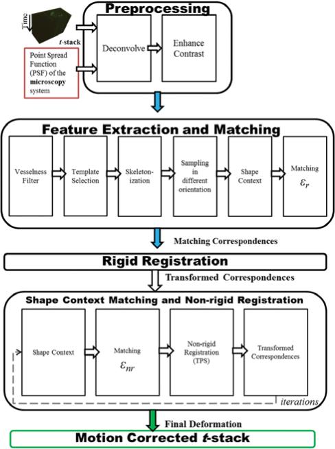
Due to the in vivo nature of the acquired images, respiration and heart pulsations in the mouse can cause severe motion artifacts and deter automatic analysis of blood flow dynamics. The first and foremost task of pursuing an automatic framework for the analysis of t-stack images for any biological system or living tissue is the removal of any movement present in these images. The goal of this article is to establish a motion-correction framework to address this task. The proposed method is applicable to any time-series microscopy image sequence that exhibits biological structures with recognizable shapes and boundaries such as vessels, dendrites, and axons. Previous work in correcting motion in microscopy images has focused on intensity based methods (Yang et al., 2008; Greenberg & Kerr, 2009; Lee et al., 2011; Lorenz et al., 2011). But, to our knowledge, a point-based method for motion correction in microscopy images has not been proposed. Points on the skeletons of the biological structures form the impetus for using a point-based registration approach. The method presented in this article is not limited to the number of frames in the t-stack. For the demonstration of this algorithmic framework, a t-stack of the vasculature in the islets of Langerhans has been used as the primary dataset and input. The method is comprised of the following parts: (1) deconvolution, (2) contrast enhancement, (3) vesselness filter, (4) template selection, (5) skeletonization, (6) sampling and binning, (7) shape contexts (SCs) and matching, (8) rigid registration, and (9) nonrigid registration using thin plate splines (TPS). A flowchart illustrating the major blocks of the algorithmic framework is shown in Figure 1.

Figure 1.

Flowchart showing the major blocks of the algorithmic framework. The primary input into this framework is the t-stack or time-series image stack acquired from a Zeiss LSM 5 LIVE microscope. The top section of the block diagram describes the involved preprocessing steps for the t-stack before the feature extraction and registration steps can occur. The middle section of the block diagram details the elements of developing a robust feature descriptor before matching correspondence pairs can be formed. These matching correspondence pairs are used in a rigid registration step to yield a transformed set of correspondence pairs, which account for large movements in t-stacks. The bottom section of the block diagram specifies the connections and the iterative flow between the nonrigid registration segment and SC matching step. The final output is the motion corrected t-stack.

Materials and Methods

Image Acquisition Procedures

Animals

Experiments involving mice were approved by and performed according to the guidelines of the Vanderbilt University Institutional Animal Care and Use Committee. The majority of the experimental procedures referred to in this article involving pancreas exteriorization and in vivo fluorescence imaging has been previously discussed in Nyman et al. (2010). Mouse insulin I promoter–green fluorescent protein (GFP) transgenic mice were courtesy of Hara and Bell from the University of Chicago (Hara et al., 2003; Quoix et al., 2007).

Pancreas Exteriorization

An intraperitoneal injection of xylazine-ketamine (20/80 mg/kg) was used to anesthetize the mice. By making an incision in the abdominal cavity, the splenic end of the pancreas was revealed. Gauze bedding was placed gently on the abdominal cavity, and the pancreas-spleen connection was fixed over the bedding. The mouse was secured prone on a heated stage, and the pancreas was in contact with the imaging window. The exposed pancreas was kept moist during imaging by occasionally adding 0.9% saline to the gauze bedding.

In Vivo Fluorescence Imaging

The LSM 5 LIVE (Carl Zeiss, Oberkochen, Germany.) line-scanning confocal laser microscope with a ×20/0.8 NA planapochromat air objective lens was used for the imaging. Considering the objective lens’ properties, this microscope system is of the paraxial form. The slit aperture was 3.20 Airy units for the vasculature channel and 2.78 Airy units for the RBC channel, for an approximately 6 μm imaging depth. These values were adjusted for each channel for optimal signal-to-noise ratio (SNR) and spatial resolution. The imaging window was 0.16–0.19 mm thick (Corning #2940-245). Using epifluorescence, islets in the exposed pancreas were identified by the GFP labeled β-cells. GFP was excited with a 488 nm diode laser, and islets were identified by emission through a 540–625 nm band-pass filter. Islets closer to the surface provided the best resolution. Tetramethylrhodamine dextran tracer [2 × 10⁶ MW, Molecular Probes (Eugene, OR, USA), dissolved to 10 mg/mL in 0.9% saline] was used to label the vasculature. On the day of imaging, RBCs from a donor mouse were labeled by osmotic shock loading with Alexa Fluor 647 hydrazide tris (triethylammonium) salt (Molecular Probes). Briefly, 200 μL of washed RBCs in 0.9% saline was added to a mixture of 35 μL Alexa Fluor 647 (2 mg/mL in distilled deionized water) and 200 μL of distilled deionized water, in a 0.5 mL Eppendorf tube. It was gently mixed by suction using a 200 μL Eppendorf pipet and allowed to incubate at room temperature for 20 min. After incubation, 31.9 μL of 10× phosphate buffered saline (Gibco, Grand Island, NY, USA) was added to the mixture, the tube gently vortexed, and the contents spun-down for 4 min at 2,000 rpm (400 g) in an Eppendorf microfuge. A portion of the supernatant was drawn off, and the labeled RBCs subsequently washed five times with 0.9% saline, each time spinning-down for 3 min at 2,000 rpm (400 g). The resulting uniformly labeled RBC solution was adjusted to 200 μL with 0.9% saline and stored at 4°C. Before the imaging experiment both the vasculature label and the labeled RBCs were equilibrated to room temperature. During the imaging experiment a one-to-one mixture of vasculature label and labeled RBCs (~50 μL each) was injected into the mouse through a carotid artery catheter.

The RBCs and vasculature labels were excited using 532 and 635 nm diode lasers, respectively, and the emission collected using 540–625 nm band-pass filters and 650 nm long-pass filters, respectively. The emissions were collected simultaneously through two detection channels leading to two-channel time-series images. All time-series scans, for analysis here, were collected at 100 frames per second (fps) for 30 s to 2 min. The frame size was 512 × 256 pixels. For each pancreatic islet, time-series scans were collected at multiple depths below the surface of the tissue, denoted by z = z₀. Each single-plane image series forms the much referred to time-series or t-stack, I(x, y, z = z₀, t) also denoted as I(x, y, t), in this article. This t-stack captures blood flow dynamics in the midst of respiratory and heart induced movements. The t-stack channel that captures the labeled vasculature is used in this motion correction framework, and the channel that captures the labeled RBCs is not used in this framework.

Image Algorithm

This section is the core of this article and seeks to elaborate on the major blocks of the algorithm shown in Figure 1. The preprocessing block, detailed in the Preprocessing section, contains the deconvolution and contrast enhancement stages. Deconvolution is used to remove artifacts caused by the optical characteristics of the microscopy system. The resulting deconvolved t-stack has much of the present noise in I(x, y, t) filtered. However, as a side effect, a slight haze contaminates the salient features, and this is addressed by enhancing the contrast.

The feature extraction and matching block is comprised of various stages—vesselness filter stage for estimating the presence of vessels, skeletonization of the vessels, template selection for performing registration, sampling and binning points along the skeletonized vessels based on the orientation of vessels, SCs for capturing this distribution of points per orientation, and perform matching of several SCs between the template and the current image frame in the t-stack based on a cost function. This matching results in homologous points or correspondences that are subsequently used in the registration block. This section is detailed in the Feature Extraction and Matching section.

The motion artifacts present in the t-stack do have a rigid and a nonrigid component; hence, the registration block is composed of these two stages. The correspondences resulting from the Feature Extraction and Matching section are used in the registration block, as described in the Registration section.

Preprocessing

Deconvolution

This first step of the preprocessing block, as shown in Figure 1, is used to restore the t-stack image, I(x, y, t), acquired by the LSM 5 LIVE system using deconvolution. The LSM 5 LIVE microscope's point spread function (PSF) contributes to the formation of I(x, y, t) (McNally et al., 1999). Deconvolution techniques can adequately remove the manifest artifacts resulting from the optics of the microscope on the t-stack (McNally et al., 1999; Verveer et al., 1999; Cannell et al., 2006; Biggs, 2010). The theoretical PSF model for this microscope has been derived for the paraxial case (Sandison & Webb, 1994; Wolleschensky et al., 2006) and for the nonparaxial case (Dusch et al., 2007). To generate the paraxial LSM 5 LIVE's PSF for RBCs and vasculature, the excitation and detection wavelengths used for highlighting RBCs and vasculature from the Image Acquisition Procedures section were appropriately substituted (Wolleschensky et al., 2006).

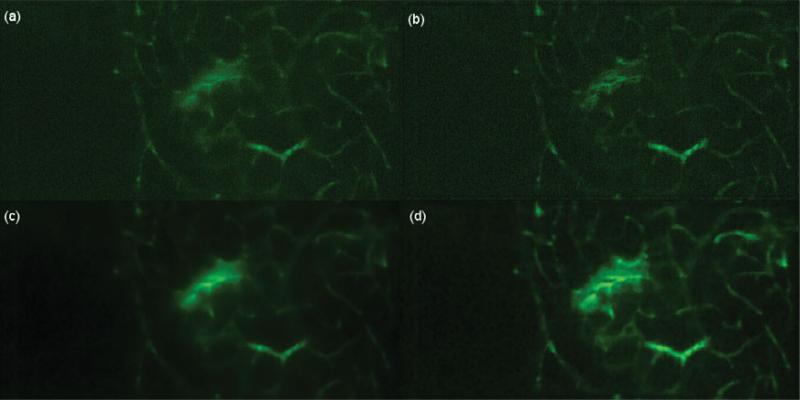
Considering the intensity values captured in the LSM 5 LIVE, images are signal-dependent and directly proportional to photon count causing the manifest noise in these images to adhere to a Poisson distribution, and therefore the Richardson-Lucy with total-variation regularization (RLTV) algorithm (Richardson, 1972; Lucy, 1974; McNally et al., 1999; Verveer et al., 1999; Dey et al., 2006) is appropriately selected. The RLTV algorithm has desirable properties, including stable convergence, ability to reduce ringing artifacts occurring at feature edges, and robustness to noise using regularization. Using the DeconvolutionLab software package available from Vonesch and Unser (2008), the RLTV algorithm with regularization parameter λ_RLTV and n_RLTV iterations was used for deconvolving I(x, y, t). The parameters, λ_RLTV and n_RLTV, used for this deconvolution step are specified in Table 1. Figure 2 shows the image restoration by deconvolution using the RLTV algorithm.

Table 1.

Fixed Values for Parameters Used in Various Stages of the Framework.

Algorithm	Variable	Description	Value/Formula
Preprocessing
Richardson-Lucy with RLTV	λ RLTV	Regularization parameter for RLTV	0.002
	n RLTV	Number of iterations for RLTV	10
Enhance contrast	cHE	Clip level for CLAHE	3
Feature Extraction and Matching
Vesselness filter	w	Scales (standard deviation) for Gaussians	1, 2, 3, 4, 5,6
	gb	Block-size for second-order Gaussian derivatives	15 × 15
	β	Control sensitivity of line filter	0.5
	c	Control sensitivity of line filter	0.5*max(Λ)
Nonmaxima suppression	rnms	Radius to consider for NMS	1.5
Hysteresis	Hysthigh	Threshold for starting a skeleton	0.05
	Hystlow	Threshold for continuing a skeleton	0.005
Sampling	θ orientations	Angle subdivision for orientation binning	τ/4
	norientations	Number of orientation bins	τ/θorientations
	ns	Number of samples per orientation	200
Shape context	Kθ	Angular bins for log-polar histogram	12 or τ/6
	Krad	Radial bins for log-polar histogram	11
	K	Total number of bins for log-polar histogram	132
	rinner	Inner-radius for log-polar histogram	1/8
	router	Outer-radius for log-polar histogram	4
	μ	Weighing parameter for cost functions	0.1
Registration
Nonrigid registration	λ	Regularization parameter for TPS	106
	γ	Annealing parameter	0.93
	nnr	Number of iterations for TPS	5

Figure 2.

Preprocessing results are shown: (a) original image showing vessels, (b) CLAHE on the original image without the deconvolution operation increases noise, (c) deconvolution, as outlined by the Preprocessing section, on the original image, and (d) CLAHE on the deconvolved image increases the appearance of salient features. Note the haze in panel c and its disappearance in panel d.

Enhance Contrast

The second step of the preprocessing block deals with the slight haze resulting from the deconvolution step. Figure 2c shows the result from the deconvolution of I(x, y, t) and the presence of the slight haze. This presence of a slight haze corrupts the saliency of features in the output image, O(x, y, z = z₀), and this can be accounted for by enhancing the contrast. Contrast-limited adaptive histogram equalization (CLAHE) is able to maintain the high spatial frequency content of the image and reduce edge shadowing effects produced by the standard adaptive histogram equalization technique (Zuiderveld, 1994; Pisano et al., 1998). In CLAHE, a user-specified maximum, called the clip-level c_HE, is imposed on the height of the local histogram and on the maximum contrast enhancement factor. Figure 2d depicts the result of CLAHE on the deconvolved image. Figure 2d is the input for the feature extraction and matching block of this motion correction methodology as illustrated in the middle section of Figure 1.

Feature Extraction and Matching

Vesselness Filter

Tubular structures, namely, vessels, can be detected, highlighted, and characterized by a “vesselness” measure using a multiscale vessel filter as described in Frangi et al. (1998). Vesselness is evaluated on each frame of the t-stack, denoted by I(x, y), where I(x, y) is the preprocessed image, i.e., it has been deconvolved and contrast enhanced as per the Preprocessing section. Eigenvalue analysis of the Hessian matrix of the image can locally extract principal directions of curvature. To compute vesselness, the image, I(x, y), is convolved with second derivatives of Gaussians at multiple scale sizes, w, to construct the Hessian matrix, H_w, defined in equation (1). In equation (1), I_xx, I_xy, I_yx, and I_yy represent the partial second derivatives of I(x, y). Multiple scales w aid in the detection of small to large vessels in I(x, y).

$$H_w=\left[\begin{array}{cc}\hfill I_{xx}\hfill & \hfill I_{xy}\hfill \\ \hfill I_{yx}\hfill & \hfill I_{yy}\hfill \end{array}\right].$$ (1)

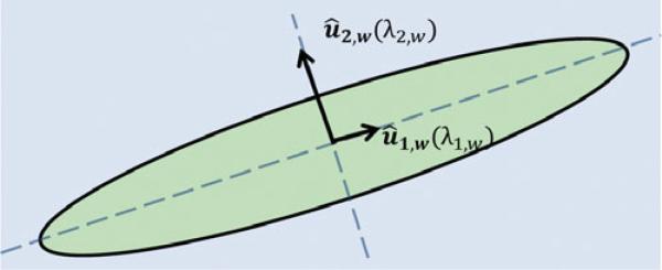
The eigenvectors, û_1,w and û_2,w, of H_w correspond to intensity variations along the principal directions of the two-dimensional (2D) tubular structure or vessel. The eigenvector û_1,w, corresponding to the eigenvalue λ_1,w, indicates the direction of the body of the vessel as it is also the direction of the minimum intensity variation. Figure 3 illustrates the extracted principal directions, û_1,w and û_2,w, of an ideal 2D tubular structure at a scale w.

Figure 3.

A 2D tubular structure or vessel has an elongated ellipse shape. The eigenvectors, depicted as black arrows, of H_w, reveal the principal directions of the vessel at scale size w. The length of these black arrows represents the absolute value of the corresponding eigenvalues. Note the smaller length of the eigenvector, û_1,w, reflecting the direction of minimum intensity variation, in light green, or the body of the vessel.

From Frangi et al. (1998), the vesselness measure or response at scale size w, V_w(x, y), can be defined as shown in equation (2). Furthermore, maximal vesselness response, V(x, y), occurs when the size of the vessel to detect approximately matches the scale size w and is shown in equation (3). The values of β, c, and the range of scale sizes for w are mentioned in Table 1. Figure 4b illustrates the result from equation (3) and is the final output of the vesselness filter. This output will be the subsequent input into the later steps of the algorithm.

$$V_w(x,y)=\left\{\begin{array}{c}\hfill 0,{\lambda }_{2,w}>0\hfill \\ \hfill \exp \left(-\frac{R_{\beta }^2}{2{\beta }^2}\right)\left(1-\exp \left(-\frac{{\Lambda }^2}{2c^2}\right)\right)\hfill \end{array}\right\},$$ (2)

where

$$\begin{array}{cc}\hfill R_{\beta }=& \frac{{\lambda }_1}{{\lambda }_2}\text{and}\Lambda ={\Vert H_w\Vert }_F=\Vert \sqrt{{\lambda }_1^2+{\lambda }_2^2}\Vert \hfill \\ \hfill V(x,y)=& {\max }_{w_{\min }\le w\le w_{\max }}\left(V_w(x,y)\right).\hfill \end{array}$$ (3)

Figure 4.

(a) A frame from the t-stack, the original preprocessed image, I(x, y), and (b) maximal vesselness filter response, V(x, y). Note that all vessels in panel a are captured in panel b.

Template Selection

To perform any registration step, a “source” and a “target” image need to be designated. Although there is no limit in the number of frames that can be analyzed with the presented method, the t-stacks used consist of approximately 3,000–12,000 frames acquired at 100 fps. Each frame's movement can be deemed independent of each other and thus form the “target” images. For the presented algorithmic framework, the manually selected template frame of the vessel-enhanced t-stack is picked as the “source” image or “template,” V₀(x, y), and the i'th frame of the vessel-enhanced t-stack, V_i(x, y), is registered to this template. The frame of the t-stack that displays the least amount of movement is selected as the template frame. Figure 5 reflects the selected template superimposed with a target frame.

Figure 5.

(a) Template frame, V₀(x, y), (b) target frame, V_i(x, y) to be registered, and (c) template, in red, superimposed with the target frame, in green. Note the large movement between the template and target frames.

Skeletonization

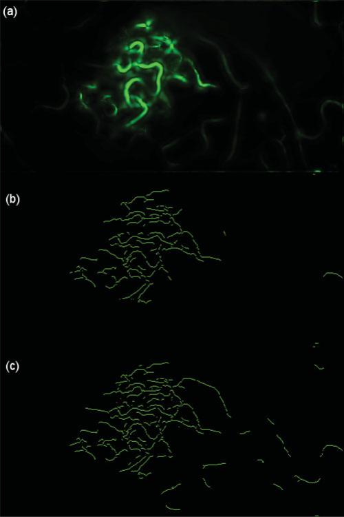
For the registration of V_i(x, y) to V₀(x, y), a neighborhood of vessel structures in V_i(x, y) should approximately match the neighborhood of vessel structures in V₀(x, y). Intuitively, the skeletonization of a vessel provides its topological description. Hence, skeletonization of all vessels present in I(x, y) will provide for a topological context, which will be utilized in the SC block of this algorithm. Given vesselness values at each pixel in I(x, y) and its corresponding eigenvector, û_2,w, the skeleton describing the topology of vessel structures can be found using non-maxima suppression (NMS) (Forsyth & Ponce, 2002). In this article, NMS aims to find local maxima in V(x, y). The vesselness response is maximal at any pixel by comparing all vesselness values along the normal directions, indicated by û_2,w and –û_2,w, around a radius r_nms. Once the local vesselness maximum in r_nms has been determined and stored, the rest of the vesselness response values in r_nms is suppressed. Typically, it is expected that the local vesselness maxima of the vessel structure will lie around the centerline of the vessel. NMS does not consider the magnitude of the determined local maxima, and this can lead to unwanted branches on the extracted skeletons of the vessels. To counter this, a hysteresis thresholding step (Forsyth & Ponce, 2002) is used to find the most significant connected vessel skeletons by starting a vessel skeleton when it satisfies a Hyst_high vesselness threshold and continuing this skeleton when it satisfies a Hyst_low vesselness threshold in an eight-connected neighborhood, where Hyst_high >> Hyst_low. The values describing r_nms, Hyst_high, and Hyst_low are given in Table 1, and the skeletonization of vessels is shown in Figure 6a.

Figure 6.

(a) The extracted skeletons of vessels for a frame of the t-stack is displaced. (b) The sampling on the vessel skeletons in four different orientations is shown, seen in different colors.

Sampling

Skeletons binned into orientations can increase robustness and reduce clutter when computing correspondences between V₀(x, y) and V_i(x, y). The skeletons of vessel structures have an associated vesselness value, V(x, y), and associated eigenvectors, û₁ and û₂. The angle between these eigenvectors can yield the local orientation of the vessel's skeleton, and this can be appropriately binned into a number of orientations, denoted by n_orientations. A user-defined angle, θ_orientations, is divided into τ to compute n_orientations, with each orientation delineated by θ_j. Once the extracted vessel skeletons have been assigned to an orientation, sampling can occur. Figure 6b exhibits the sampling process with n_s sample points in four orientation bins on the vessels’ skeleton. Table 1 describes the values of n_s and θ_orientations used in this framework, and the effects of these parameters is discussed in the Results section.

Shape Contexts

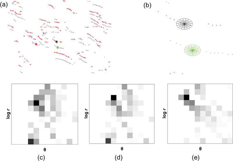
To perform registration, homologous points need to be determined, and one method to achieve this is to construct feature descriptors. Several of these feature descriptors can be constructed for both the template, V₀(x, y) in θ_j, and the target frame, V_i(x, y) in θ_j, and a matching scheme based on a cost function can be used to obtain correspondence pairs, which will be used in the subsequent registration steps. Let V₀ be the samples obtained on the template, V₀(x, y), and V_i be the samples obtained on the target frame, V_i(x, y). To build the feature descriptor, SC descriptor, proposed by Belongie et al. (2002), is suitable as it encodes a vessel's representative sample points in a neighborhood. The SC descriptor bins spatial relationships between points in a neighborhood as a log-polar histogram with a total of K bins. This gives each sample point, seen in Figure 7b, a description based on its neighboring sample points, which forms the context of the sample point. The SC descriptor is compact, intrinsically translational and scale invariant, highly discriminative, robust to the presence of outliers, and robust to deformations. An example of the SC descriptor is illustrated in green and black in Figure 7b. The log-polar histogram centered at a point, p, a sample point on the skeleton of a vessel, maps the population of points contained in the several bins of the log-polar histogram into a feature vector as shown in Figures 7c–7e. In essence, the SC descriptor is a feature vector in the form of a coarse histogram describing the relative coordinates of the set of points in the neighborhood of p. The various parameters used to construct SCs are also described in Table 1.

Figure 7.

(a) Sample points for one orientation, θ_j, for the template (in red) and a target frame from t-stack (in blue) and three log-polar histograms centered is shown, (b) zoomed in view of the log-polar histograms, black log-polar histogram belongs to the template, while the green and red log-polar histograms belong to the target frame, (c) the SC (dark = large value) for the black log-polar histogram, (d) the SC for the green log-polar histogram, and (e) the SC for the red log-polar histogram. The axes of the SCs are log(radius) versus θ. Note the similarity of the histograms of images c and d.

From Figures 7c–7e, it is apparent that Figure 7e is dissimilar to Figures 7c and 7d, and to quantify this dissimilarity, a representative cost function needs to be developed. Since SCs are histograms, a χ² statistic can be used as a cost function, C_sc (Belongie et al., 2002).

Consider a point, p_V0 on V₀, and a point p_Vi on V_i, and their associated K-bin normalized SCs, h(p_V0; k) and h(p_Vi; k), then C_sc(p_V0, p_Vi) can be defined as indicated in equation (4), and this measures the similarity between the feature vectors of p_V0 and p_Vi.

$$C_{sc}(p_{V0},p_{Vi})=\frac{1}{2}\sum _{k=1}^K\frac{{[h(p_{V0};k)-h(p_{Vi};k)]}^2}{h(p_{V0};k)+h(p_{Vi};k)}.$$ (4)

For the purposes of motion correction, C_sc is not sufficient to characterize the dissimilarity of SCs under severe clutter, and hence an additive cost function term is needed. A continuity cost term, C_cont, ensures that two adjacent points, p_V0 and q_V0, on the template, V₀, are also adjacent points on the target frame, V_i (Thayananthan et al., 2003). This notion is explained in Figure 8 and is specified in equation (5). In equation (5), neighboring template points p_V0 and q_V0 should map to p_Vi = φ(p_V0) and q_Vi = φ(q_V0) on the target frame, respectively, where p_Vi and q_Vi are neighbors as well on the target frame. The function φ maps points in the template, V₀, to the target frame, V_i, and the computation of φ is explained in the matching stage of the algorithm. The total cost, C_total, to minimize per orientation bin, θ_j, during the matching operation of this algorithm is given in equation (6), where μ is a weighing parameter.

$$C_{cont}(V_0,V_i)={\Sigma }_{\forall p,q\in V_0}\Vert \phi \left(p_{V0}\right)-\phi \left(q_{V0}\right)\Vert$$ (5)

$$C_{total}\left({\theta }_j\right)=(1-\mu )\ast C_{sc}(V_0,V_i)+\mu \ast C_{cont}(V_0,V_i).$$ (6)

Figure 8.

This diagram shows the intuition behind C_cont. The distances between adjacent p_V0 and q_V0 points should be similar to the distances of the neighboring p_Vi and q_Vi points.

Matching

Minimizing the total cost in equation (6) per orientation bin, θ_j, can be assessed as solving a weighted bipartite matching problem (Belongie et al., 2002), wherein each point, p_V0, on the template, V₀, gets solely matched to one point, p_Vi, on the target frame, V_i. This assignment problem for generating correspondence pairs, (p_V0, p_Vi), can be solved using the well-established Hungarian method (Kuhn, 1955; Papadimitriou & Steiglitz, 1998), also known as Kuhn-Munkres assignment algorithm. This method produces φ, the previously discussed mapping function. One drawback of the Hungarian method is that it performs a one-to-one assignment for all sample points, inclusive of outliers, from the target V_i to the sample points in V₀. Henceforth, to dispose of anomalous correspondence pairs, (p_V0, p_Vi), the Euclidean distance between p_V0 and p_Vi, denoted as d(p_V0, p_Vi), is computed, and the pair is rejected if d(p_V0, p_Vi) > ε. The value of ε is user-defined, and two kinds of ε are used in this algorithmic framework, ε_r for rigid registration and ε_nr for nonrigid registration. Finally, the set of matched correspondence pairs for each θ_j are sent to the registration block of this algorithmic framework.

Registration

Rigid Registration

From the Feature Extraction and Matching section, the sets of matched correspondence pairs for all orientations θ_j are accumulated into one pool of correspondence pairs, and this pool is the input into the rigid registration step. Rigid registration transforms the matched points from the target to the template using the least-squares method (Fitzpatrick et al., 2000). This transformation explains the global movements in the frames of t-stack; however, to account for local movements, a nonrigid registration refinement step is used.

Nonrigid Registration

The pool of transformed correspondences from the rigid registration step is the input into the nonrigid registration stage, as described in the bottom section of Figure 1. The nonrigid registration refinement used is based on TPS (Bookstein, 1989). The smoothness of the resulting deformation field is controlled by a regularization parameter, λ (Rohr et al., 2001), which is annealed over n_nr iterations using γ annealing parameter, described in Table 1. From Figure 1, the input pool is split up into its respective orientations, θ_j; SCs are recomputed for each θ_j; matching with ε_nr criterion is executed for each θ_j; and matched correspondence pairs for all orientations are accumulated to compose an updated pool of correspondences. TPS with an annealed regularization parameter is carried out on the updated pool to result in a new pool of transformed correspondence pairs, the new input. This refinement procedure is repeated for n_nr iterations. Regularized TPS on the final pool of transformed correspondence pairs, V_f, yields a final deformation field that is utilized in correcting the local motion present in t-stacks.

Results

It is evident that the ground truth for the manifest in vivo motion of the biological specimen in these t-stacks is unknown. Thus, to quantify the motion correction performed with this framework, the stability of the t-stack based on normalized cross-correlation (NCC) is used. Often, NCC is used in template matching, and the peak of the NCC plot displays where the template matches a test image. The location of this peak is an offset or distance of how much the test image needs to be moved to fully match the template; this is denoted by d_NCC. Once the test image has been moved by the offset, the resulting d_NCC will be 0, and this can be understood as the test image being stable against the template. In the presented use of this framework, with the template and each frame of the t-stack of the same dimensions, a motion corrected t-stack's stability can be measured by the total d_NCC. Since the raw t-stacks are noisy, the vessel-enhanced t-stacks are used for computing NCC and d_NCC. In addition to quantifying the stability of the motion correction, a qualitative analysis based on maximum intensity projection (MIP) of the outcomes from the proposed registration framework is detailed in this section to show the effectiveness of the framework. Both quantitative and qualitative results need to be examined to assess the performance of the motion correction performed on a dataset.

The parameter values in Table 1 were picked empirically and were held constant for all datasets. The pillars of this motion correction framework are the sample points on the vessel structures, SC descriptors constructed on these sample points, correspondence matching, and registration. The sampling of points on the vessel structures depends on acceptable hysteresis results. Good hysteresis results lead to adequate samples for constructing meaningful SC descriptors, which is used in the matching and registration steps. In effect, the parameters in Table 1 were picked to produce acceptable hysteresis results. Figure 9 displays the effect of using two different hyst_high values. For the t-stacks, the hysteresis thresholds were selected such that majority of the vessels were skeletonized, over all datasets. The effect of lack of skeletonization of the vessels leads to less smooth deformation fields and poor motion correction. The number of orientations, n_orientations, used in binning the samples in the sampling stage was picked as 4 to represent 45° intervals. SC descriptors are built per θ_j and matched accordingly. In our datasets, selecting more than four orientations, θ_j, for binning of samples leads to suboptimal construction of SCs. This is attributed to the lack of a distribution of sample points, in a θ_j, to capture in the SC descriptor. Suboptimal SCs are less unique and meaningful in the matching stage and thus will yield poor registration results. The parameters for SCs help capture the distribution of the sample points in a log-polar plot. Increasing the angular bins (K_θ) from 12 and radial bins (K_rad) from 11 had no effect on the motion correction. However, less than 12 angular bins affected the granularity of the log-polar histogram leading to poor matching of correspondences, which lead to suboptimal motion correction. For the nonrigid registration step, regularization parameter (λ) and annealing parameter (λ) were changed until the resulting deformation field was sufficiently smooth and regularized, and MIP was sharp for all datasets. Lower λ and λ values resulted in overfitting of the deformation fields to the correspondences and yielded poor motion correction results.

Figure 9.

(a) A vessel-enhanced image frame of Dataset 6, (b) skeletonizations of vessels with hyst_high = 0.1, and (c) skeletonizations of vessels with hyst_high = 0.05 compares the effect of the upper hysteresis threshold, hyst_high, on skeletonizations of vessels. Samples are generated directly on these skeletonizations and used in building SC descriptors. (c) Sampling on skeletonizations of vessels in a majority of the image frame area will lead to the construction of meaningful SCs and smoother deformation fields. A lack of sampling on absent skeletonizations in most of the image frame in b will lead to abnormal deformation fields. See the discussion in the Results section.

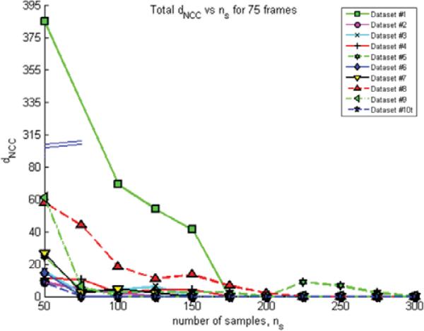
The number of samples, n_s, per orientation bin, θ_j, can significantly affect the performance of the presented algorithm. The value of n_s directly corresponds to the construction of meaningful SC descriptors. Once hysteresis produces acceptable results, samples need to be generated in the sampling stage and n_s determines the number of SC descriptors used to perform correspondence matching and, subsequently, registration. Lower values of n_s will yield nonunique SCs and will compromise the matching stage. The number of samples, n_s, was fixed as 200 per θ_j for all datasets used in this algorithmic framework. This value was determined by running 75 frames of all t-stack datasets, sweeping n_s from 50 to 300 in increments of 25. The metric, d_NCC, was computed for each dataset and n_s combination and is shown as a graph in Figure 10. When the total d_NCC is minimized, motion correction has been successful and overall, from Figure 10, a value of n_s equal to 200 is sufficient to perform motion correction for all datasets presented.

Figure 10.

This graph shows the number of samples, n_s, being swept from 50 to 300 in increments of 25, versus d_NCC values for each dataset. The specific value of n_s that minimizes d_NCC leads to successful motion correction, and this value of n_s is the minimum number of samples per θ_j required to achieve the motion correction. From the graph, a value of n_s = 200 is sufficient to perform motion correction on all the datasets presented.

Table 2 shows the values for two parameters, ε_r and ε_nr, categorized for “less,” “moderate,” and “most” movement present in t-stacks. The user selects the category of the movement for the entire t-stack image dataset, and the appropriate ε_r and ε_nr are picked for the motion correction.

Table 2.

Values of Parameters Based on User-Selected Category Describing the Motion.

	Less Movement	Moderate Movement	Most Movement
ε r	15	25	45
ε nr	4	4	8

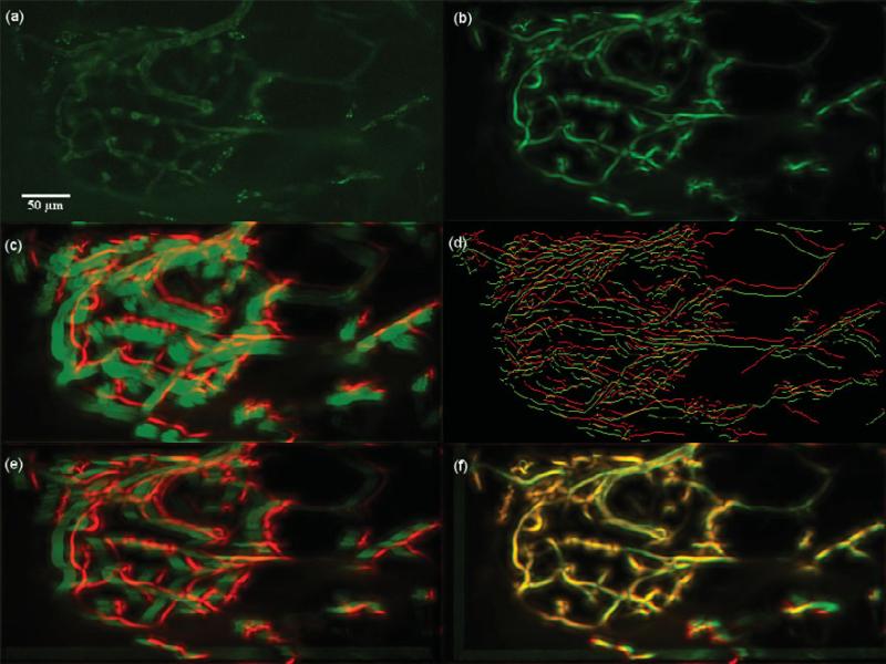
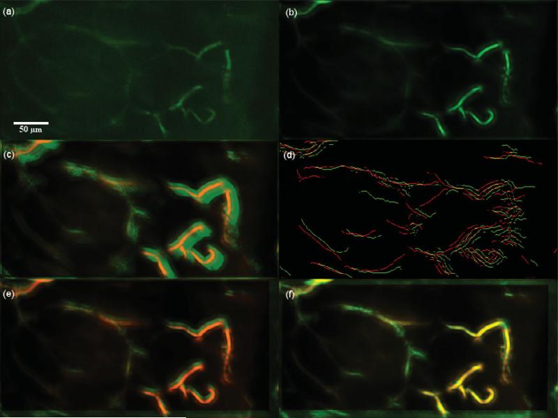
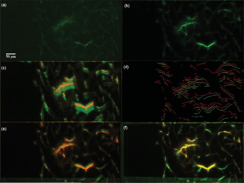
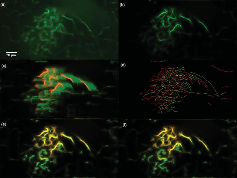
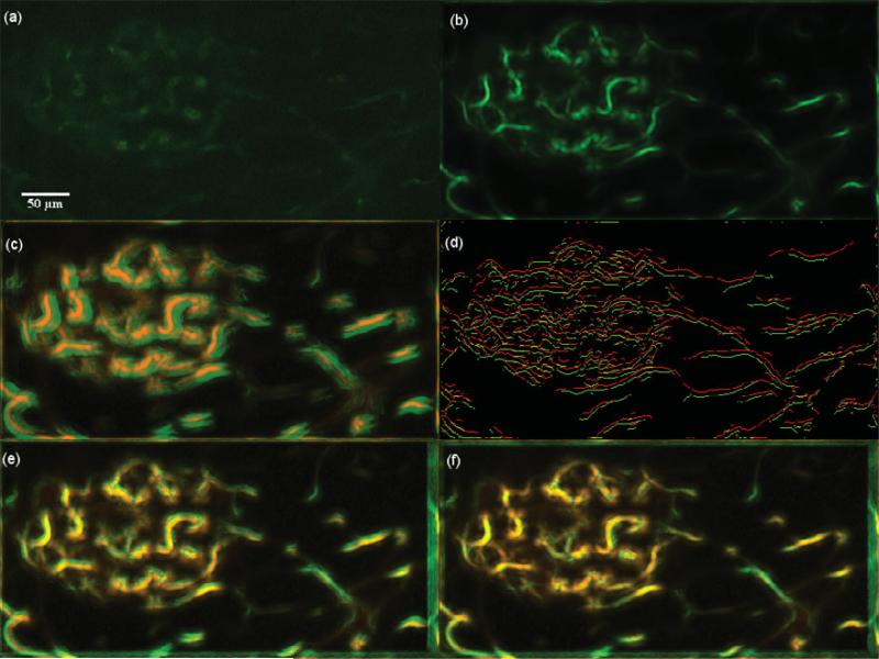
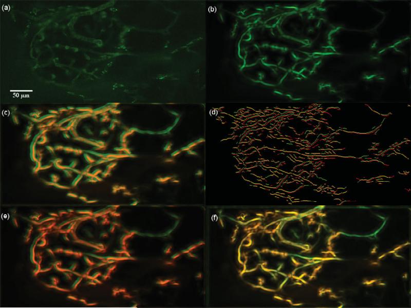
In the presented framework, motion correction can be regarded as being based on a template matching scheme. Since NCC is an intensity-based method used for template matching, it also forms a baseline for comparing the presented point-based motion correction using SC descriptors (Lee et al., 2011). Since the raw t-stack exhibits noise, the vessel-enhanced t-stack is used as the input into the baseline. Table 3 quantifies the stability of the motion correction based on the mean d_NCC of the vessel-enhanced t-stacks and n_s = 200. From Table 3, we note that the stability of the time-series sequences greatly improves, and the in vivo motion has been corrected with the use of the presented algorithm based on SCs. The intensity-based NCC correction, the baseline, corrects the in vivo motion as well, but it is limited to rigid-motion and fails to correct for nonrigid in vivo motion in the t-stack. This can be seen in the qualitative results for Datasets 2, 3, and 8. The baseline is not able to correct most of Dataset 1 because there is too much clutter in the vessel-enhanced image. The presented framework corrects the motion in Dataset 1, and a comparison is shown in Figures 11e–f. Since Dataset 6 primarily exhibits rigid motion, both the baseline and the presented algorithm perform equally well and is illustrated in Figures 16e and 16f. The comparison between the baseline and the algorithm is shown qualitatively for all datasets in Figures 11e, 11f–20e, 20f.

Table 3.

Comparison of Mean NCC Peak Offset Distance, d_NCC (μm), for Motion Correction.

Dataset	Number of Frames	Pixel Size (μm)	Category	Uncorrected	NCC Corrected	Present Method (This work)
1	375	0.89	Most	19.809	15.237	0.00522
2	600	0.78	Most	4.7422	2.3131	0.10943
3	450	1.24	Most	6.6937	2.9485	0.01210
4	450	1.24	Most	6.3661	0.23448	0.01849
5	375	0.78	Moderate	1.9053	1.4000	0
6	600	1.04	Most	11.492	0	0.00734
7	600	1.04	Most	12.114	0.03467	0
8	450	0.89	Moderate	4.5431	1.3916	0.05631
9	225	0.89	Less	2.9519	2.7812	0
10t	75	0.78	Most	4.9196	2.4232	0

Figure 11.

Dataset 1, 375 frames, “most” movement at depth z₀ = 11.625 μm. (a) A frame of the original t-stack. (b) The template used for performing motion correction. (c) The template (red channel) superimposed on the MIP (green channel) of the uncorrected t-stack. (d) Hysteresis results of the template superimposed with a frame of the uncorrected t-stack. (e) The template (red channel) superimposed on the MIP of the motion corrected t-stack (green channel) using the baseline algorithm. (f) The template (red channel) superimposed on the MIP of the motion corrected t-stack (green channel) using the presented algorithm; notice the near perfect overlap in yellow and the sharpness of all the vessels. The baseline is not able to correct the motion because of increased clutter of vasculature in panel e.

Figure 16.

Dataset 6, 600 frames,“most” movement at depth z₀ = 25.000 μm. (a) A frame of the original t-stack. (b) The template used for performing motion correction. (c) The template (red channel) superimposed on the MIP (green channel) of the uncorrected t-stack. (d) Hysteresis results of the template superimposed with a frame of the uncorrected t-stack. (e) The template (red channel) superimposed on the MIP of the motion corrected t-stack (green channel) using the baseline algorithm. (f) The template (red channel) superimposed on the MIP of the motion corrected t-stack (green channel) using the presented algorithm; notice the near perfect overlap in yellow and the sharpness of all the vessels. Dataset 6 primarily exhibits rigid motion and both the baseline and the presented algorithm perform well as seen in images e and f.

Figure 20.

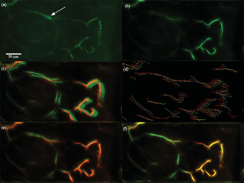
Dataset 10^t, 75 frames, “most” movement at depth z₀ = 30.925 μm. These 75 frames are a part of Dataset 2. (a) A frame of the original t-stack. The manually manipulated brightness of a vessel to simulate Ca²⁺ imaging is indicated by the arrow. (b) The template used for performing motion correction. (c) The template (red channel) superimposed on the MIP (green channel) of the uncorrected t-stack. (d) Hysteresis results of the template superimposed with a frame of the uncorrected t-stack. (e) The template (red channel) superimposed on the MIP of the motion corrected t-stack (green channel) using the baseline algorithm. (f) The template (red channel) superimposed on the MIP of the motion corrected t-stack (green channel) using the presented algorithm; notice the near perfect overlap in yellow and the sharpness of all the vessels. Video 4 displays the motion correction and the robustness of the algorithm to brightness changes.

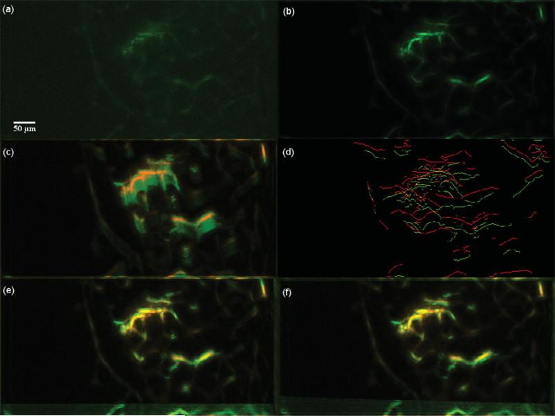
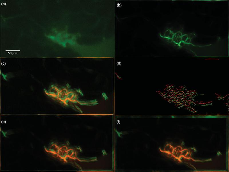
The qualitative evaluation of motion correction is based on MIPs. The MIP of the frames of the t-stack's uncorrected motion against its template will be more smeared, less sharp, and have less overlap with the template. On the other hand, when the motion is corrected, the MIP of the frames of the t-stack against its template will be sharp and overlap almost completely with the template. The qualitative results show MIPs of uncorrected motion, NCC-based correction, and the presented algorithmic framework. These qualitative results are shown in Figures 11–20 and are best viewed in color. Figures 11d–20d display the hysteresis results between the template and an image frame of the respective t-stack on which the sampling process will occur. These samples are used in constructing SCs on both the template and the image frame to perform registration. Videos 1–2 show the motion correction for “most” movement in Datasets 2–7. Video 3 shows the motion correction for “moderate” movement in Dataset 8.

To measure the robustness of this motion correction framework to transient illumination such as in the case of Ca²⁺ imaging, we manipulated the brightness of a fraction of the imaged blood vessels in a subset of the raw data. Parts of the vessels in the raw Dataset 2 were manually selected, and the brightness was multiplied by 1.5 to simulate transient signals and is referred to as Dataset 10^t in Table 3. The framework is robust to transient signals, and this can be seen in the motion correction presented in Figure 20 and Video 4 for Dataset 10^t.

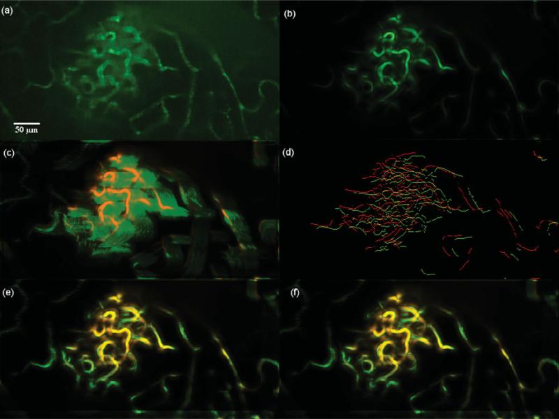
Though the qualitative and quantitative results from the motion correction framework are encouraging, there are certain cases where the motion correction results are suboptimal. These cases, specifically Dataset 4, shown in Figure 14, often occur when the t-stack's depth, signified by z₀, is too large or deep, and this can lead to low signal-to-background ratio (SBR) and SNR in the acquired t-stack images. Another case that yields suboptimal results is Data-set 5, shown in Figure 15, in which most of the vesselness response is contained in a small portion of the image frame. These cases can cause issues in the vesselness response resulting in lack of skeletonizations of vessels in certain areas of the image frame, which affects the sampling process detrimentally. Subsequently, the sampling process on these skeletonizations produces sample points in certain areas of the image frame and a lack of sample points in other areas.This lack of sample points in other areas of the image frame will affect the computed deformation field during the registration stage. In a sense, the computed deformation field is predominantly guided by a set of correspondence pairs representing a small portion of the image frame, and this yields some abnormal movements in the empty areas of the image as correspondence pairs in those areas are lacking. The resulting deformation field is over-fitted, less smooth, and less regularized. Datasets 4 and 5 display this notion qualitatively. The quantitative metric, d_NCC, considers the peak offset distance between the NCC of the template and the image frame, and is not able to capture the nonsmooth deformations in areas where the vesselness response is poor. This deficiency is apparent when comparing quantitative and qualitative results for Datasets 4 and 5, Figures 14 and 15, respectively. Hence, the evaluation of the presented motion correction framework needs to be judged qualitatively and quantitatively.

Figure 14.

Suboptimal case. Dataset 4, 450 frames, “most” movement at depth z₀ = 40.400 μm. (a) A frame of the original t-stack. (b) The template used for performing motion correction. (c) The template (red channel) superimposed on the MIP (green channel) of the uncorrected t-stack. (d) Hysteresis results of the template superimposed with a frame of the uncorrected t-stack. (e) The template (red channel) superimposed on the MIP of the motion corrected t-stack (green channel) using the baseline algorithm. (f) The template (red channel) superimposed on the MIP of the motion corrected t-stack (green channel) using the presented algorithm. From panel d, the sampling process is compromised by the poor hysteresis response leading to a not so sharp overlap of the MIPs of template and the motion corrected t-stack.

Figure 15.

Suboptimal case. Dataset 5, 450 frames, “moderate” movement at depth z₀ = 20.450 μm. (a) A frame of the original t-stack. (b) The template used for performing motion correction. (c) The template (red channel) superimposed on the MIP (green channel) of the uncorrected t-stack. (d) Hysteresis results of the template superimposed with a frame of the uncorrected t-stack. (e) The template (red channel) superimposed on the MIP of the motion corrected t-stack (green channel) using the baseline algorithm. (f) The template (red channel) superimposed on the MIP of the motion corrected t-stack (green channel) using the presented algorithm. The lack of density of points in various parts of the image leads to a lack of samples in those areas, a lack of SCs to use for correspondences and registration, finally leading to a less smooth deformation field. This causes the MIP to be less sharp, yielding suboptimal results.

The presented motion correction framework is programmed in MATLAB 7.10.0 (MathWorks Inc., Framingham, MA, USA, R2010a), executed on eight-core AMD Opteron machines with 10GB RAM, and on average takes 7 h to correct 3,000 frames. The code is available upon request.

Discussion

The presented motion correction framework is the first step of a suite of algorithms aimed to compute local and global changes in velocities of RBCs in the islets of Langerhans, with changes in glucose and other pharmacological treatments, to gain an insight into blood flow dynamics and restriction points. The motion correction framework is able to correct the motion in the t-stacks regardless of the number of frames because each frame is registered to a template independently. This allows for future parallelization of the framework as each frame can be sent to a core processor for motion correction. The framework is mainly limited by the acquisition depth, z₀, of the t-stack because of low SBR and low SNR, and this makes biological structures less visible. Currently, n_s is fixed for all orientations, θ_j, and the user needs to select the overall category of the motion in the time-series sequence as “most,” “moderate,” and “less.” This reduces the burden of parameter searching for the user. Once the motion is corrected in the t-stacks, labeled RBCs can be tracked through the vessels merely based on their location, and their velocity can be computed by analyzing the RBC movement through vessel architecture. From the framework, vesselness response is known in the t-stack and a 2D connectivity algorithm executed on this vesselness response can generate a vessel architecture map. For the three-dimensional (3D) image stack acquired from the Zeiss LSM 5 LIVE, a similar motion correction framework can be executed, and a 3D connectivity scheme on the vessels can extract vessel architecture of the islet. Though this framework was exclusively tested on these Zeiss LSM 5 LIVE time series images, it can be used for images captured from intravital microscopy and other forms of microscopy images that exhibit in vivo motion of the biological specimen. The vesselness filter response was used in the feature extraction block of the presented algorithm, but an edge map of the image content can also be used. In essence, registration or motion correction in microscopy images, where the image content exemplifying any shape or structure that can be skeletonized, can be performed using the presented framework based on SCs.

SUMMARY

Shape contexts are employed in shape recognition by building feature descriptors and comparing them to a database of known shapes such as alphabets (Belongie et al., 2002; Mori et al., 2005). Shape contexts also aid in the formulation of an automatic feature vector of a point and its neighboring points. This notion is accompanied by the vesselness filter to create robust descriptors employed in finding matching correspondence pairs between a template and a target image, and the performed registration step on the correspondence pairs corrects the motion. The practical point-based technique discussed in this article is novel to the microscopy field and can be applied to several types of microscopy images content of which exhibits shapes and structures.

Figure 12.

Dataset 2, 600 frames,“most” movement at depth z₀ = 30.925 μm. (a) A frame of the original t-stack. (b) The template used for performing motion correction. (c) The template (red channel) superimposed on the MIP (green channel) of the uncorrected t-stack. (d) Hysteresis results of the template superimposed with a frame of the uncorrected t-stack. (e) The template (red channel) superimposed on the MIP of the motion corrected t-stack (green channel) using the baseline algorithm. (f) The template (red channel) superimposed on the MIP of the motion corrected t-stack (green channel) using the presented algorithm; notice the near perfect overlap in yellow and the sharpness of all the vessels. Video 1 illustrates the motion correction for this dataset.

Figure 13.

Dataset 3, 400 frames,“most” movement at depth z₀ = 30.425 μm. (a) A frame of the original t-stack. (b) The template used for performing motion correction. (c) The template (red channel) superimposed on the MIP (green channel) of the uncorrected t-stack. (d) Hysteresis results of the template superimposed with a frame of the uncorrected t-stack. (e) The template (red channel) superimposed on the MIP of the motion corrected t-stack (green channel) using the baseline algorithm. (f) The template (red channel) superimposed on the MIP of the motion corrected t-stack (green channel) using the presented algorithm; notice the near perfect overlap in yellow and the sharpness of all the vessels. Video 2 illustrates the motion correction for this dataset.

Figure 17.

Dataset 7, 600 frames,“most” movement at depth z₀ = 35.050 μm. (a) A frame of the original t-stack. (b) The template used for performing motion correction. (c) The template (red channel) superimposed on the MIP (green channel) of the uncorrected t-stack. (d) Hysteresis results of the template superimposed with a frame of the uncorrected t-stack. (e) The template (red channel) superimposed on the MIP of the motion corrected t-stack (green channel) using the baseline algorithm. (f) The template (red channel) superimposed on the MIP of the motion corrected t-stack (green channel) using the presented algorithm; notice the near perfect overlap in yellow and the sharpness of all the vessels.

Figure 18.

Dataset 8, 450 frames,“most” movement at depth z₀ = 29.300 μm. (a) A frame of the original t-stack. (b) The template used for performing motion correction. (c) The template (red channel) superimposed on the MIP (green channel) of the uncorrected t-stack. (d) Hysteresis results of the template superimposed with a frame of the uncorrected t-stack. (e) The template (red channel) superimposed on the MIP of the motion corrected t-stack (green channel) using the baseline algorithm. (f) The template (red channel) superimposed on the MIP of the motion corrected t-stack (green channel) using the presented algorithm; notice the near perfect overlap in yellow and the sharpness of all the vessels. Video 3 illustrates the motion correction for this dataset.

Figure 19.

Dataset 9, 225 frames, “less” movement at depth z₀ = 11.625 μm. (a) A frame of the original t-stack. (b) The template used for performing motion correction. (c) The template (red channel) superimposed on the MIP (green channel) of the uncorrected t-stack. (d) Hysteresis results of the template superimposed with a frame of the uncorrected t-stack. (e) The template (red channel) superimposed on the MIP of the motion corrected t-stack (green channel) using the baseline algorithm. (f) The template (red channel) superimposed on the MIP of the motion corrected t-stack (green channel) using the presented algorithm; notice the near perfect overlap in yellow and the sharpness of all the vessels.

REFERENCES

- Belongie S, Malik J, Puzicha J. Shape matching and object recognition using shape contexts. IEEE T Pattern Anal. 2002;24:509–522. [Google Scholar]
- Biggs DS. 3D deconvolution microscopy. In: Robinson JP, editor. Current Protocols in Cytometry. John Wiley & Sons, Inc.; Hoboken, NJ: 2010. pp. 1–20. Chap. 12, Unit 12.19. [DOI] [PubMed] [Google Scholar]
- Bookstein FL. Principal warps: Thin-plate splines and the decomposition of deformations. IEEE T Pattern Anal. 1989;11:567–585. [Google Scholar]
- Cannell MB, McMorland A, Soeller C. Image enhancement by deconvolution. In: Pawley J, editor. Handbook of Biological Confocal Microscopy. Springer Press; New York: 2006. pp. 488–500. [Google Scholar]
- Dey N, Blanc-Feraud L, Zimmer C, Roux P, Kam Z, Olivo-Marin J-C, Zerubia J. Richardson-Lucy algorithm with total variation regularization for 3D confocal microscope deconvolution. Microsc Res Tech. 2006;69:260–266. doi: 10.1002/jemt.20294. [DOI] [PubMed] [Google Scholar]
- Dusch E, Dorval T, Vincent N, Wachsmuth M, Genovesio A. Three-dimensional point spread function model for line-scanning confocal microscope with high-aperture objective. J Microsc. 2007;228:132–138. doi: 10.1111/j.1365-2818.2007.01844.x. [DOI] [PubMed] [Google Scholar]
- Fitzpatrick JM, Hill DLG, Maurer CR. Image registration. In: Sonka M, Fitzpatrick JM, editors. Handbook of Medical Imaging. II. SPIE Press; Bellingham, WA: 2000. pp. 447–514. Chap. 8. [Google Scholar]
- Forsyth DA, Ponce J. Computer Vision: A Modern Approach. Prentice Hall; Upper Saddle River, NJ: 2002. Edge detection. pp. 230–236. Chap. 8. [Google Scholar]
- Frangi AF, Niessen WJ, Vincken KL, Viergever MA. Multiscale vessel enhancement filtering. In: Wells WM, Colchester A, Delp S, editors. MICCAI'98: Medical Image Computing and Computer-Assisted Intervention, Lecture Notes in Computer Science. Springer Verlag; Berlin: 1998. pp. 130–137. [Google Scholar]
- Greenberg DS, Kerr JND. Automated correction of fast motion artifacts for two-photon imaging of awake animals. J Neurosci Methods. 2009;176:1–15. doi: 10.1016/j.jneumeth.2008.08.020. [DOI] [PubMed] [Google Scholar]
- Hara M, Wang X, Kawamura T, Bindokas VP, Dizon RF, Alcoser SY, Magnuson MA, Bell GI. Transgenic mice with green fluorescent protein-labeled pancreatic beta-cells. Am J Physiol Endocrinol Metab. 2003;284:E177–E183. doi: 10.1152/ajpendo.00321.2002. [DOI] [PubMed] [Google Scholar]
- Kuhn HW. The Hungarian Method for the assignment problem. Nav Res Logist Q. 1955;2:83–97. [Google Scholar]
- Lee J, Srinivasan V, Radhakrishnan H, Boas DA. Motion correction for phase-resolved dynamic optical coherence tomography imaging of rodent cerebral cortex. Opt Express. 2011;19:21258–21270. doi: 10.1364/OE.19.021258. [DOI] [PMC free article] [PubMed] [Google Scholar]
- Lorenz KS, Salama P, Dunn KW, Delp EJ. Digital correction of motion artifacts in microscopy image sequences collected from living animals using rigid and nonrigid registration. J Microsc. 2011;245:148–160. doi: 10.1111/j.1365-2818.2011.03557.x. [DOI] [PMC free article] [PubMed] [Google Scholar]
- Lucy LB. An iterative technique for the rectification of observed distributions. Astron J. 1974;79:745. [Google Scholar]
- McNally JG, Karpova T, Cooper J, Conchello JA. Three-dimensional imaging by deconvolution microscopy. Methods. 1999;19:372–385. doi: 10.1006/meth.1999.0873. [DOI] [PubMed] [Google Scholar]
- Miyake T, Murakami T, Ohtsuka A. Incomplete vascular casting for scanning electron microscope study of the microcirculatory patterns in the rat pancreas. Arch Histol Cytol. 1992;55(4):397–406. doi: 10.1679/aohc.55.397. [DOI] [PubMed] [Google Scholar]
- Mori G, Belongie S, Malik J. Efficient shape matching using shape contexts. IEEE T Pattern Anal. 2005;27:1832–1837. doi: 10.1109/TPAMI.2005.220. [DOI] [PubMed] [Google Scholar]
- Nyman LR, Ford E, Powers AC, Piston DW. Glucose-dependent blood flow dynamics in murine pancreatic islets in vivo. Am J Physiol Endocrinol Metab. 2010;298:E807–E814. doi: 10.1152/ajpendo.00715.2009. [DOI] [PMC free article] [PubMed] [Google Scholar]
- Papadimitriou CH, Steiglitz K. Combinatorial Optimization: Algorithms and Complexity. Dover Publications; Mineola, NY: 1998. Weighted matching. pp. 248–254. Chap. 11. [Google Scholar]
- Pisano ED, Zong S, Hemminger BM, DeLuca M, Johnston RE, Muller K, Braeuning MP, Pizer SM. Contrast limited adaptive histogram equalization image processing to improve the detection of simulated spiculations in dense mammograms. J Digit Imaging. 1998;11:193–200. doi: 10.1007/BF03178082. [DOI] [PMC free article] [PubMed] [Google Scholar]
- Quoix N, Cheng-Xue R, Guiot Y, Herrera PL, Henquin J-C, Gilon P. The GluCre-ROSA26EYFP mouse: A new model for easy identification of living pancreatic alpha-cells. FEBS Lett. 2007;581:4235–4240. doi: 10.1016/j.febslet.2007.07.068. [DOI] [PubMed] [Google Scholar]
- Richardson WH. Bayesian-based iterative method of image restoration. J Opt Soc Am. 1972;65:55–59. [Google Scholar]
- Rohr K, Stiehl HS, Sprengel R, Buzug TM, Weese J, Kuhn MH. Landmark-based elastic registration using approximating thin-plate splines. IEEE T Med Imag. 2001;20:526–534. doi: 10.1109/42.929618. [DOI] [PubMed] [Google Scholar]
- Sandison DR, Webb WW. Background rejection and signal-to-noise optimization in confocal and alternative fluorescence microscopes. Appl Optic. 1994;33:603–615. doi: 10.1364/AO.33.000603. [DOI] [PubMed] [Google Scholar]
- Suckale J, Solimena M. Pancreas islets in metabolic signaling—Focus on the beta-cell. Front Biosci. 2008;13:7156–7171. doi: 10.2741/3218. [DOI] [PubMed] [Google Scholar]
- Thayananthan A, Stenger B, Torr PHS, Cipolla R. Shape context and chamfer matching in cluttered scenes.. Proceedings of IEEE Conference on Computer Vision and Pattern Recognition; Madison, WI. June 2003.2003. pp. 127–133. [Google Scholar]
- Verveer PJ, Gemkow MJ, Jovin TM. A comparison of image restoration approaches applied to three-dimensional confocal and wide-field fluorescence microscopy. J Microsc. 1999;193:50–61. doi: 10.1046/j.1365-2818.1999.00421.x. [DOI] [PubMed] [Google Scholar]
- Vonesch C, Unser M. A fast thresholded landweber algorithm for wavelet-regularized multidimensional deconvolution. IEEE T Imag Process. 2008;17:539–549. doi: 10.1109/TIP.2008.917103. [DOI] [PubMed] [Google Scholar]
- Wolleschensky R, Zimmermann B, Kempe M. High-speed confocal fluorescence imaging with a novel line scanning microscope. J Biomed Optic. 2006;11:064011. doi: 10.1117/1.2402110. [DOI] [PubMed] [Google Scholar]
- Yang S, Kohler D, Teller K, Cremer T, Le Baccon P, Heard E, Eils R, Rohr K. Nonrigid registration of 3-D multichannel microscopy images of cell nuclei. IEEE T Imag Process. 2008;17:493–499. doi: 10.1109/TIP.2008.918017. [DOI] [PubMed] [Google Scholar]
- Zuiderveld K. Graphic Gems IV. Academic Press; San Diego, CA: 1994. Contrast limited adaptive histogram equalization. pp. 474–485. [Google Scholar]
Associated Data
This section collects any data citations, data availability statements, or supplementary materials included in this article.